Star formation rate and metallicity of damped Lyman-$\alpha$ absorbers in cosmological SPH simulations

Abstract

We study the distribution of the star formation rate (SFR) and metallicity of damped Lyman-$\alpha$ absorbers (DLAs) in the redshift range $z=0-4.5$ using cosmological smoothed particle hydrodynamics (SPH) simulations of the $\Lambda$ cold dark matter model. Our simulations include standard radiative cooling and heating with a uniform UV background, star formation, supernova (SN) feedback, as well as a phenomenological model for feedback by galactic winds. The latter allows us to examine, in particular, the effect of galactic outflows on the distribution of the SFR and metallicity of DLAs. We employ a “conservative entropy” formulation of SPH which alleviates numerical overcooling effects that affected earlier simulations. In addition, we utilise a series of simulations of varying boxsize and particle number to investigate the impact of numerical resolution on our results.

We find that there is a positive correlation between the projected stellar mass density and the neutral hydrogen column density (${\rm N_{{\rm HI}}}$) of DLAs for high ${\rm N_{{\rm HI}}}$ systems, and that there is a good correspondence in the spatial distribution of stars and DLAs in the simulations. The evolution of typical star-to-gas mass ratios in DLAs can be characterised by an increase from about 2 at $z=4.5$ to 3 at $z=3$, to 10 at $z=1$, and finally to 20 at $z=0$. We also find that the projected SFR density in DLAs follows the Kennicutt law well at all redshifts, and the simulated values are consistent with the recent observational estimates of this quantity by Wolfe, Prochaska, & Gawiser (2003a, b). The rate of evolution in the mean metallicity of simulated DLAs as a function of redshift is mild, and is consistent with the rate estimated from observations. The predicted metallicity of DLAs is generally sub-solar in our simulations, and there is a significant scatter in the distribution of DLA metallicity for a given ${\rm N_{{\rm HI}}}$. However, we find that the median metallicity of simulated DLAs is close to that of Lyman-break galaxies, and is higher than the values typically observed for DLAs by nearly an order of magnitude. This discrepancy with observations could be due to an inadequate treatment of the SN feedback or the multiphase structure of the gas in our current simulations. Alternatively, the current observations might be missing the majority of the high metallicity DLAs due to selection effects.

1 Introduction

Damped Lyman-$\alpha$ absorbers (defined as quasar absorption systems with column density ${\rm N_{{\rm HI}}}>2\times 10^{20}\rm cm^{-2}$) have similar neutral hydrogen column density as galactic disks in the Local Universe. They are high concentrations of neutral gas which could form stars and eventually evolve into galaxies that we see today (Wolfe et al., 1986). While the most numerous absorbers are those with low column densities, the high column densities of DLAs more than compensate for their relative paucity when the relative contribution to the total neutral hydrogen (Hi  ) mass density is considered. It is thought that DLAs dominate the Hi  gas content of the Universe at $z\sim 3$ (Lanzetta, 1993; Wolfe et al., 1995; Storrie-Lombardi & Wolfe, 2000), and thus they are serving as an important reservoir of neutral gas for star formation at high redshift. Therefore, studying the physical properties of DLAs, such as the distribution of their star formation rates and metallicity, will provide us with important complementary information to those provided by the emitted light from stars in high-redshift galaxies.

It has become clear from recent observational (e.g. Adelberger et al., 1998; Steidel et al., 1999) and theoretical (e.g. Mo & Fukugita, 1996; Baugh et al., 1998; Mo, Mao, & White, 1999; Katz, Hernquist & Weinberg, 1999; Kauffmann et al., 1999; Nagamine, 2002; Weinberg, Hernquist, & Katz, 2002) studies of Lyman-break galaxies (LBGs) at $z\sim 3-4$, that the assembly of galaxies is actively going on at $z\sim 3$, consistent with what is expected from the hierarchical structure formation paradigm based on a cold dark matter (CDM) model. The star formation rates of LBGs at $z=3-4$ are now commonly observed using emission lines such as H$\alpha$, or by fitting the entire spectrum with population synthesis models (e.g. Shapley et al., 2001). These measurements of SFRs typically give values of $\sim 50~{}\rm M_{\odot}\rm yr^{-1}$ for LBGs, allowing one to place a lower limit on the cosmic star formation rate by combining the information on the SFR and number density of LBGs.

Furthermore, many theoretical and observational studies suggest that the cosmic star formation rate rises towards high redshift, even beyond $z=3$ (e.g. Pascarelle, Lanzetta, & Fernández-Soto, 1998; Blain et al., 1999; Nagamine et al., 2001; Lanzetta et al., 2002; Springel & Hernquist, 2003b; Hernquist & Springel, 2003). Therefore, the conversion of gas into stars is taking place at a significant rate in these high-redshift galaxies at $z\geq 3$. Studying this conversion process can help us understand the galaxy formation better, and possibly constrain structure formation scenarios such as the hierarchical CDM models.

However, estimating the star formation rate in DLAs has proven to be very difficult, because the stellar counterparts of DLAs cannot be detected in emission due to their faintness. Wolfe, Prochaska, & Gawiser (2003a, b) have therefore adopted a different approach and recently estimated the SFR in DLAs in the redshift range $z=3-4$ by utilising the Cii^∗ 1335.7 absorption line. They infer the heating rate by equating it to the cooling rate measured from Cii^∗ absorption. Since the heating rate is proportional to the SFR, they can then deduce the SFR from the estimated heating rate. The values of SFR they measure by this method roughly agree with the Kennicutt law (Kennicutt, 1998) with some scatter. The robustness of this technique still needs to be tested with future observations, but it is encouraging that observers are making progress towards a ‘direct’ measurement of the SFR in DLAs.

On the other hand, there is a wealth of observational data on the chemical abundances of DLAs from detailed studies of quasar absorption line spectra (see Pettini 2003 for an excellent review). DLAs are generally inferred to be metal poor at all redshifts (e.g. Pettini et al., 1994; Lu et al., 1996; Pettini et al., 1999; Prochaska & Wolfe, 1999). The column density-weighted mean abundance of zinc is measured to be $\sim 1/13$ of solar ($\left\langle[{\rm Zn/H}]\right\rangle=-1.13$), which suggests that DLA galaxies (i.e. galaxies in which DLAs arise) are at early stages of their chemical evolution. The measured values of [Zn/H] span more than an order of magnitude at each redshift, and the chemical enrichment appears to proceed at different rates in different DLAs. The metallicity distribution of DLAs peaks at a value in-between those of halo and thick-disk stars of the Milky Way (Fig. 8 of Pettini 2003; Wyse & Gilmore 1995; Laird et al. 1988), suggesting that the kinematics of DLAs should be closer to stellar haloes and bulges than to rotationally supported disks. This finding is at odds with the proposal by Prochaska & Wolfe (1998) that most DLAs are large disks with rotational velocities in excess of 200 $\rm km\,s^{-1}$. An interesting fact is that there is little evidence for any redshift evolution in the metallicity of DLAs (Pettini et al., 1999; Prochaska & Wolfe, 2000, 2002), despite the fact that most analytic models of global chemical evolution of the Universe predict substantial evolution in metallicity as a function of time (e.g. Pei & Fall, 1995). However, most recently Prochaska et al. (2003) have detected mild evolution with a significantly larger sample of DLAs. It is interesting to see if full cosmological simulations agree with observations or analytic models of global chemical evolution, and what they predict in detail for DLA metallicities.

Theoretical understanding of the physical properties of DLAs still remains primitive. Several semi-analytic models of DLAs and their chemical evolution exist (e.g. Pei & Fall, 1995; Kauffmann, 1996; Jimenez et al., 1999; Mo, Mao, & White, 1999; Prantzos & Boissier, 2000; Somerville, Primack, & Faber, 2001; Maller, Prochaska, Somerville, & Primack, 2001, 2002; Lanfranchi & Friaca, 2003), but they often neglect the effect of galaxy mergers, infall of gas, outflows due to supernovae, and the interaction with the intergalactic medium (IGM). These dynamical processes are expected to have significant influence on the chemical evolution of DLAs, and it would therefore be ideal to study the chemical evolution of DLAs with full cosmological hydro-simulations which treat all of these effects dynamically and self-consistently. The earlier numerical studies of Gardner et al. (1997a,b; 2001) for example did not address the chemical evolution of DLAs in detail.

Run	Boxsize	${N_{\rm p}}$	$m_{\rm DM}$	$m_{\rm gas}$	$\epsilon$	$z_{\rm end}$	wind
R3	3.375	$2\times 144^{3}$	$9.29\times 10^{5}$	$1.43\times 10^{5}$	0.94	4.00	strong
R4	3.375	$2\times 216^{3}$	$2.75\times 10^{5}$	$4.24\times 10^{4}$	0.63	4.00	strong
O3	10.00	$2\times 144^{3}$	$2.42\times 10^{7}$	$3.72\times 10^{6}$	2.78	2.75	none
P3	10.00	$2\times 144^{3}$	$2.42\times 10^{7}$	$3.72\times 10^{6}$	2.78	2.75	weak
Q3	10.00	$2\times 144^{3}$	$2.42\times 10^{7}$	$3.72\times 10^{6}$	2.78	2.75	strong
Q4	10.00	$2\times 216^{3}$	$7.16\times 10^{6}$	$1.10\times 10^{6}$	1.85	2.75	strong
Q5	10.00	$2\times 324^{3}$	$2.12\times 10^{6}$	$3.26\times 10^{5}$	1.23	2.75	strong
D4	33.75	$2\times 216^{3}$	$2.75\times 10^{8}$	$4.24\times 10^{7}$	6.25	1.00	strong
D5	33.75	$2\times 324^{3}$	$8.15\times 10^{7}$	$1.26\times 10^{7}$	4.17	1.00	strong
G4	100.0	$2\times 216^{3}$	$7.16\times 10^{9}$	$1.10\times 10^{9}$	12.0	0.00	strong
G5	100.0	$2\times 324^{3}$	$2.12\times 10^{9}$	$3.26\times 10^{8}$	8.00	0.00	strong

Table 1: Simulations employed in this study. The box-size is given in units of $h^{-1}{\rm\,Mpc}$, ${N_{\rm p}}$ is the particle number of dark matter and gas (hence $\times\,2$), $m_{\rm DM}$ and $m_{\rm gas}$ are the masses of dark matter and gas particles in units of $h^{-1}{\rm M_{\odot}}$, respectively, $\epsilon$ is the comoving gravitational softening length in units of $h^{-1}{\rm\,kpc}$, and $z_{\rm end}$ is the ending redshift of the simulation. The value of $\epsilon$ is a measure of spatial resolution. From the top to the bottom row, we refer to R3 & R4 collectively as ‘R-series’, the next 5 runs (O3 to Q5) are called ‘Q-series’, D4 & D5 are called ‘D-series’, and G4 & G5 are called ‘G-series’. The ‘strong-wind’ simulations form a subset of the runs analysed by Springel & Hernquist (2003b).

In our previous paper (Nagamine, Springel, & Hernquist, 2003), we studied the abundance of DLAs using a series of cosmological SPH simulations with varying resolution and feedback strength. We showed that the $\Lambda$CDM model is able to account for the observed abundance of DLAs at redshift $z=3-4.5$ quite well. Another important conclusion of our study was that earlier numerical work overestimated the DLA abundance significantly due to insufficient numerical resolution, lack of efficient feedback processes, and inaccuracies introduced in cooling processes when conventional formulations of SPH are used, giving rise to an overcooling problem. In our simulation methodology, we avoided these numerical difficulties by using a novel version of SPH (Springel & Hernquist, 2002) that is based on integrating the entropy as an independent thermodynamic variable (e.g. Lucy, 1977; Hernquist, 1993), and which takes variations of the SPH smoothing lengths self-consistently into account.

In this paper, we focus on the overall distribution of the star formation rate and metallicity of DLAs in the redshift range $z=0-4.5$. We are interested in how these quantities appear in our new SPH simulations, in light of our refined modelling of star formation and feedback by galactic winds, and our new formulation of SPH. In particular, we will examine the dependence of our results on feedback strength, and also investigate the influence of numerical resolution on the physical properties of DLAs.

The evolution of metallicity in DLAs has previously been studied with a cosmological hydro-simulation by Cen et al. (2002), using an Eulerian code with a fixed mesh-size. The methodology of this simulation is very different from ours, but it is clearly interesting to compare their results to what we find. We discuss this comparison in Section 9.

The paper is organised as follows. In Section 2, we briefly describe the novel features of our simulations, putting particular emphasis on the star formation model and the treatment of metal production. We show a few examples of visual representations of haloes and associated physical quantities in Section 3. We then discuss the distribution of Hi  column density as a function of halo mass in Section 4, projected stellar mass density in Section 5, projected SFR density in Section 6, and projected metallicity of DLAs in Section 7. The evolution of the mean metallicity is described in Section 8. Finally, we discuss the implications of our work in Section 9.

2 Simulations

We analyse a large set of cosmological SPH simulations that differ in box size, mass resolution and feedback strength, as summarised in Table 1. In particular, we consider box sizes ranging from 3.375 to $100h^{-1}{\rm\,Mpc}$ on a side, with particle numbers between $2\times 144^{3}$ and $2\times 324^{3}$, allowing us to probe gaseous mass resolutions in the range $4.2\times 10^{4}$ to $1.1\times 10^{9}\,h^{-1}{\rm M}_{\odot}$. These simulations are partly taken from a study of the cosmic star formation history by Springel & Hernquist (2003b), supplemented by additional runs with weaker or no galactic winds. The joint analysis of this series of simulations allows us to significantly broaden the range of spatial and mass-scales that we can probe compared to what is presently attainable within a single simulation.

There are three main new features of our simulations. First, we use a “conservative entropy” formulation of SPH (Springel & Hernquist, 2002). This approach has several advantages over conventional versions of SPH. Since the energy equation is written with the entropy as the independent thermodynamic variable, rather than the thermal energy, the ‘p dV’ term is not evaluated explicitly, reducing noise from smoothed estimates of e.g. the density. By including terms involving derivatives of the density with respect to the particle smoothing lengths, this approach explicitly conserves entropy (in regions without shocks), as well as momentum and energy, even when smoothing lengths evolve adaptively, avoiding the problems noted by e.g. Hernquist (1993). Furthermore, this formulation moderates the overcooling problem present in earlier formulations of SPH (see also Yoshida et al., 2002; Pearce et al., 1999; Croft et al., 2001).

Second, we employ an effective sub-resolution model described by Springel & Hernquist (2003a) to treat star formation and its regulation by supernovae feedback in the dense interstellar medium (ISM). In this model, the highly overdense gas of the ISM is pictured to be a two-phase fluid consisting of cold clouds in pressure equilibrium with a hot ambient phase. Each gas particle represents a statistical mixture of these phases. Cold clouds grow by radiative cooling out of the hot medium, and this material forms the reservoir of baryons available for star formation. We assume that star formation takes place on a characteristic time-scale $t_{\star}$, and that a mass fraction $\beta$ of these stars are short-lived and instantly die as supernovae so that the local SFR is:

$$\frac{{\rm d}\rho_{\star}}{{{\rm d}t}}=(1-\beta)\frac{\rho_{c}}{t_{\star}},$$ (1)

where $\rho_{c}$ is the gas density of the cold cloud phase. The value of $\beta$ is determined by the initial mass function of the stellar population, and here we adopt $\beta=0.1$. The star formation time-scale $t_{\star}$ is taken to be proportional to the local dynamical time of the gas:

$$t_{\star}(\rho)=t_{0}^{\star}\left(\frac{\rho}{\rho_{\rm th}}\right)^{-1/2},$$ (2)

where the value of $t_{0}^{\star}=2.1~{}\rm Gyr$ is chosen to match the Kennicutt law (1998). Because of its density dependence, the star formation time-scale becomes short in very high density regions, approximately modelling intense starburst activity. In our model, this parameter simultaneously determines a threshold density $\rho_{\rm th}$, above which the multiphase structure in the gas, and hence star formation, is allowed to develop. This physical density is $8.6\times 10^{6}h^{2}\rm M_{\odot}{\rm kpc}^{-3}$ for all simulations in this study, corresponding to a comoving baryonic overdensity of $7.7\times 10^{5}$ at $z=0$. See Springel & Hernquist (2003a) for a description for how $\rho_{\rm th}$ is determined self-consistently within the model.

In our simulation code, the mass of a new star particle is fixed to $m_{\star}=m_{0}/N_{g}$, where $m_{0}$ is the initial mass of each gas particle, and $N_{g}$ (which we take to be 2 here) is the number of “generations” of stars each gas particle may spawn. New star particles are created probabilistically with expectation value consistent with the current SFR of each gas particle.

Once star formation occurs, the resulting supernova explosions are assumed to deposit energy into the hot gas with an average of $\epsilon_{\rm SN}=4\times 10^{48}\rm ergs~{}\rm M_{\odot}^{-1}$ for each solar mass of stars formed, or 0.4% of the canonical SN energy of $10^{51}~{}\rm ergs$. The efficiency of SN energy feedback is often described as the ratio of the returned SN energy to the rest mass energy of the star formed, in which case our SN feedback efficiency translates to $\epsilon_{\rm SN}/\rm M_{\odot}c^{2}=2.2\times 10^{-6}$. The heating rate due to SN is

$$\left.\frac{{\rm d}}{{\rm d}t}(\rho_{h}u_{h})\right|_{\rm SN}=\epsilon_{\rm SN}\frac{{\rm d}\rho_{\star}}{{\rm d}t}=\beta u_{\rm SN}\frac{\rho_{c}}{t_{\star}},$$ (3)

where $u_{\rm SN}\equiv(1-\beta)\beta^{-1}\epsilon_{\rm SN}$ is the ‘SN energy scale’ corresponding to a ‘SN temperature’ of $T_{\rm SN}=2\mu u_{\rm SN}/3k\simeq 10^{8}\,{\rm K}$, and $\rho_{h}$ and $u_{h}$ are the density and thermal energy of the hot phase of the gas, respectively.

We assume that SN explosions also evaporate the cold clouds, and transfer cold gas back into the ambient hot phase. This can be described as

$$\left.\frac{{\rm d}\rho_{c}}{{\rm d}t}\right|_{\rm EV}=A\beta\frac{\rho_{c}}{t_{\star}}.$$ (4)

The efficiency parameter $A$ has the density dependence

$$A(\rho)=A_{0}\left(\frac{\rho}{\rho_{\rm th}}\right)^{-4/5},$$ (5)

following McKee & Ostriker (1977). The value of $A_{0}$ is fixed to 1000 by requiring $T_{\rm SN}/A_{0}=10^{5}$ K. This evaporation process of cold clouds establishes a tight self-regulation mechanism for star formation in the ISM, where the ambient hot medium quickly evolves towards an equilibrium temperature equal to

$$u_{h}=\frac{u_{\rm SN}}{A+1}+u_{c}$$ (6)

in a time-scale shorter than the star formation time-scale. Therefore, it is a good approximation to assume that the condition of self-regulated star formation always holds. We can then avoid treating the mass exchange between the hot and cold phases explicitly. This simplifies the code, makes it faster, and reduces its memory consumption. In this ‘effective’ model, which is adopted for all the runs used in the present study, the thermal energy of the hot phase is simply given by equation (6), and that of the cold phase is fixed to the equivalent of $T_{c}=1000~{}\rm K$. Our result does not depend on the choice of $T_{c}$ as long as $T_{c}\ll 10^{4}~{}\rm K$, because the current code does not include molecular hydrogen or metal line cooling which would act at temperatures below $10^{4}~{}\rm K$. The mass fraction in the cold clouds for the particles in the multiphase medium can be computed by

$$x\equiv\frac{\rho_{c}}{\rho}=1+\frac{1}{2y}-\sqrt{\frac{1}{y}+\frac{1}{4y^{2}}},$$ (7)

where

$$y\equiv\frac{t_{\star}\Lambda_{\rm net}(\rho,u_{h})}{\rho[\beta u_{\rm SN}-(1-\beta)u_{c}]}.$$ (8)

Here, $\Lambda_{\rm net}(\rho,u)$ is the usual cooling function.

If the physical density of a gas particle is lower than $\rho_{\rm th}$, the particle represents ordinary gas in a single phase. In this case, the neutral hydrogen mass of the particle can be computed as

$$m_{\rm HI}=N_{\rm h}\cdot X_{\rm H}\cdot m_{\rm gas}\quad(\rho<\rho_{\rm th}),$$ (9)

where $X_{\rm H}=0.76$ is the primordial mass fraction of hydrogen, and $N_{\rm h}$ is the number density of neutral hydrogen atoms in units of the total number density of hydrogen nuclei. The quantity $N_{\rm h}$ is computed by solving the ionisation balance as a function of density and current UV background flux. If the gas density is higher than $\rho_{\rm th}$, the gas particle represents multiphase gas, such that the mass of neutral hydrogen can be computed as

$$m_{\rm HI}=x\cdot X_{\rm H}\cdot m_{\rm gas}\quad(\rho>\rho_{\rm th}),$$ (10)

where $x$ is the mass fraction of cold clouds given by equation (7).

The simulation also keeps track of metal enrichment, and the dynamical transport of metals by the motion of the gas particles. Metals are produced by stars and returned into the gas by SN explosions. The mass of metals returned is $\Delta M_{Z}=y_{\star}\Delta M_{\star}$, where $y_{\star}=0.02$ is the yield, and $\Delta M_{\star}$ gives the mass of newly formed long-lived stars. Assuming that each gas element behaves as a closed box locally, with metals being instantaneously mixed between cold clouds and the ambient hot gas, the metallicity $Z=M_{Z}/M_{g}$ of a star-forming gas particle increases during one timestep $\Delta t$ by

$$\Delta Z=(1-\beta)y_{\star}\,x\,\frac{\Delta t}{t_{\star}}.$$ (11)

When a star particle is generated, it simply inherits the metallicity of its parent gas particle.

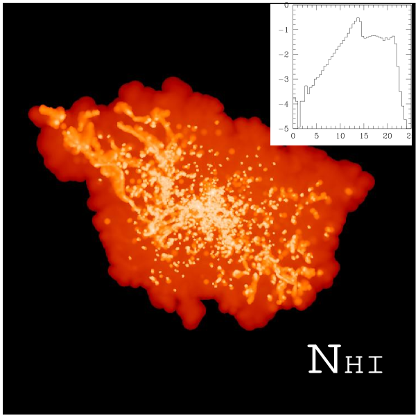
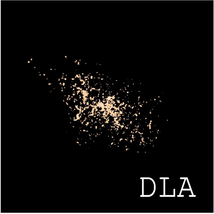
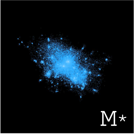
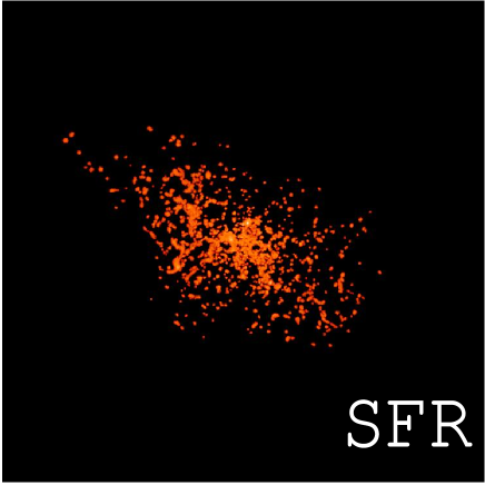
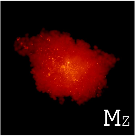
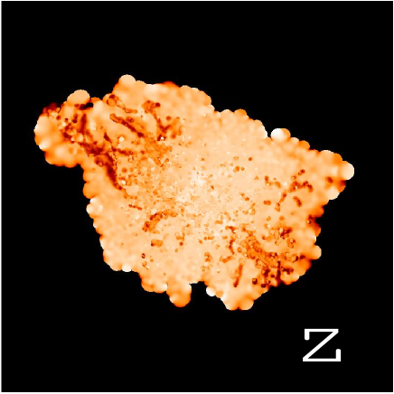
Figure 1: Projected spatial distribution of various quantities (all in log scale) for the most massive halo of mass $M_{\rm halo}=1.7\times 10^{12}h^{-1}\rm M_{\odot}$ at $z=3$ in the ‘Q5’-run. From top left to bottom right: ${\rm N_{{\rm HI}}}$, DLAs ($\log{\rm N_{{\rm HI}}}>20.3$), stellar surface mass density, SFR surface density, metal mass surface density, gas metallicity. The size of each panel is comoving $\pm 457h^{-1}{\rm\,kpc}$ from the centre of the halo. The inset in the top left panel shows the probability distribution function of lines-of-sight (${\rm d}n/{\rm d}\log{\rm N_{{\rm HI}}}$) for this halo as a function of $\log{\rm N_{{\rm HI}}}$. One can see that the majority of the red region is occupied by lines of sight with $11<\log{\rm N_{{\rm HI}}}<15$.

Finally, the third important feature of our simulations is a phenomenological model for galactic winds, which we introduced in order to study the effect of outflows on DLAs, galaxies, and the intergalactic medium (IGM). In this model, gas particles are stochastically driven out of the dense star-forming medium by assigning an extra momentum in random directions, with a rate and magnitude chosen to reproduce mass-loads and wind-speeds similar to those observed. The wind mass-loss rate $\dot{M}_{W}$ is assumed to be proportional to the star formation rate, and the wind carries a fixed fraction $\chi$ of SN energy:

$$\dot{M}_{W}=\eta\dot{M}_{\star},$$ (12)

and

$$\frac{1}{2}\dot{M}_{W}v_{w}^{2}=\chi\epsilon_{\rm SN}\dot{M}_{\star}.$$ (13)

We adopted a fixed value of $\eta=2$, and explored two values of $\chi$, a ‘weak wind model’ with $\chi=0.25$, and a ‘strong wind model’ with $\chi=1.0$ . Solving for the wind velocity from the above two equations, the wind models correspond to speeds of $v_{w}=242~{}\rm km\,s^{-1}$ and $484~{}\rm km\,s^{-1}$, respectively. This wind energy is not included in $\epsilon_{\rm SN}$ discussed above, so in our simulations $(1+\chi)\epsilon_{\rm SN}$ is the total SN energy returned into the gas.

Most of our simulations employ the ‘strong’ wind model, but for the $10\,h^{-1}{\rm Mpc}$ box (runs O3, P3, Q3, Q4, Q5; collectively called ‘Q-series’) we also varied the wind strength. Therefore, this Q-series can be used to study both the effect of numerical resolution and the consequences of feedback from galactic winds. The runs in the other simulation series then allow the extension of the strong wind results to smaller scales (‘R-Series’), or to larger box-sizes and hence lower redshift (‘D-’ and ‘G-Series’). Our naming convention is such that runs of the same model (box-size and included physics) are designated with the same letter, with an additional number specifying the particle resolution.

Our calculations include a uniform UV background radiation field of a modified Haardt & Madau (1996) spectrum, where reionisation takes place at $z\simeq 6$ (see Davé et al., 1999), as suggested by observations (e.g. Becker et al., 2001) and radiative transfer calculations of the impact of the stellar sources in our simulations on the IGM (e.g. Sokasian et al., 2003). The radiative cooling and heating rate is computed as described by Katz et al. (1996). The adopted cosmological parameters of all runs are $(\Omega_{\rm m},\Omega_{\Lambda},\Omega_{\rm b},\sigma_{8},h)=(0.3,0.7,0.04,0.9,0.7)$. The simulations were performed on the Athlon-MP cluster at the Center for Parallel Astrophysical Computing (CPAC) at the Harvard-Smithsonian Center for Astrophysics, using a modified version of the parallel GADGET code (Springel, Yoshida & White, 2001).

3 Visual representations

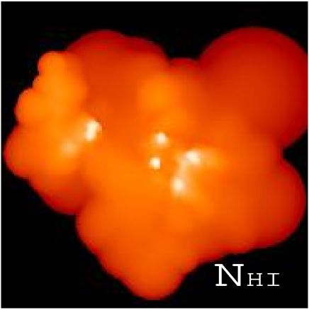
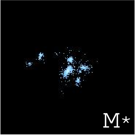
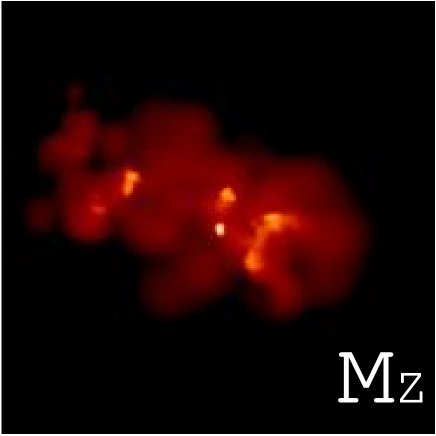
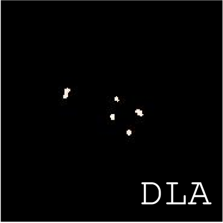
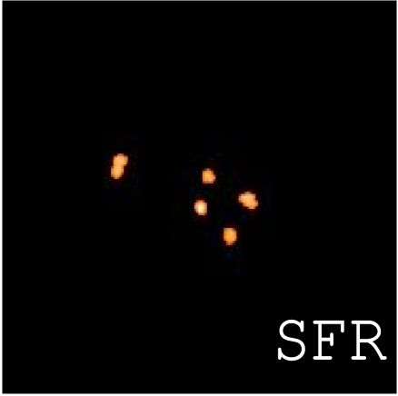
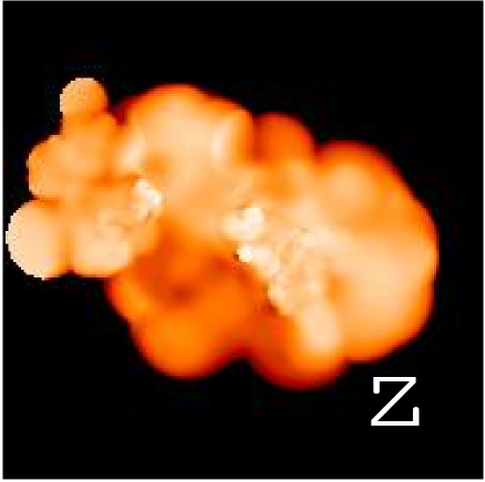
Figure 2: Projected spatial distribution of various quantities for a halo of mass $M_{\rm halo}=2.6\times 10^{10}h^{-1}\rm M_{\odot}$ at $z=3$ in the ‘Q5’-run. Left column: ${\rm N_{{\rm HI}}}$ (top) and DLAs (bottom). Middle column: stellar surface mass density (top) and SFR surface density (bottom). Right column: metal mass surface density (top) and gas metallicity (bottom). The size of each panel is comoving $\pm 112h^{-1}{\rm\,kpc}$ from the centre of the halo.

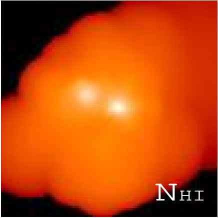
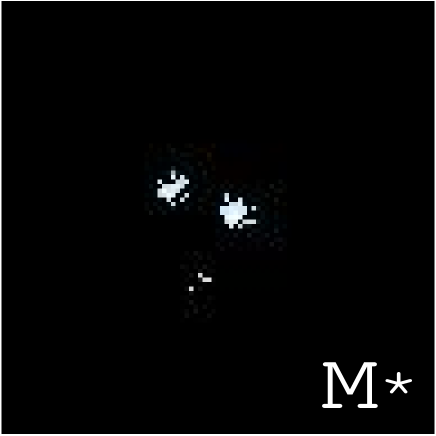
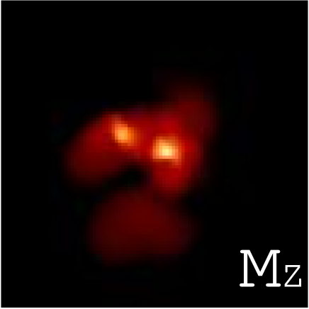
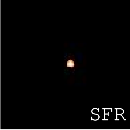
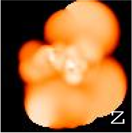
Figure 3: Projected spatial distribution of various quantities for a halo of mass $M_{\rm halo}=2.4\times 10^{9}h^{-1}\rm M_{\odot}$ at $z=3$ in the ‘Q5’-run. The size of each panel is comoving $\pm 57h^{-1}{\rm\,kpc}$ from the centre of the halo. The graph on the top left shows the probability distribution function of lines-of-sight (${\rm d}n/{\rm d}\log{\rm N_{{\rm HI}}}$) for this halo and the one shown in Figure 2 as a function of $\log{\rm N_{{\rm HI}}}$. One can see that the majority of the orange region is occupied by lines-of-sight with $11<\log{\rm N_{{\rm HI}}}<16$, which could be observed in the Ly-$\alpha$ forest. The other panels are ordered in the same way as in Figure 2.

In Figures 1, 2, and 3, we show the spatial distribution of the following quantities for 3 representative haloes in our highest resolution simulation at $z=3$ (‘Q5’-run): neutral hydrogen column density ${\rm N_{{\rm HI}}}$, DLAs (simply setting a threshold of $\log{\rm N_{{\rm HI}}}>20.3$ to the total ${\rm N_{{\rm HI}}}$), projected stellar mass surface density, projected star formation rate surface density, projected metal mass surface density, and projected metallicity. The size and the mass of each halo is given in the caption. The pixel size of the picture is taken to be the gravitational softening length of the simulation, which is $1.23\,h^{-1}{\rm\,kpc}$ for the ‘Q5’-run. We defer a discussion of quantitative results to the following sections and here simply summarise notable features of each figure.

Figure 1: This halo is the most massive one at $z=3$ ($M_{\rm halo}=1.7\times 10^{12}h^{-1}\rm M_{\odot}$), which presumably evolves into a group of galaxies at lower redshift. Note that this is a very rare halo at $z=3$. With our limited boxsize of ${\rm L_{box}}=10h^{-1}{\rm\,Mpc}$, only a few such massive haloes (which have roughly the space density of Lyman-break galaxies) can exist in our simulation box. The neutral hydrogen gas distribution in this halo is very extended, and the DLAs are widely distributed within the halo, but with a trend of higher concentration towards the centre. Obviously, the DLA cross-section of this halo is very high compared to lower mass haloes (see Figure 2 of Nagamine, Springel, & Hernquist, 2003). The inset in the top left panel shows the probability distribution function of sight-lines (${\rm d}n/{\rm d}\log{\rm N_{{\rm HI}}}$) for this halo as a function of $\log{\rm N_{{\rm HI}}}$. One can see that the majority of the red region is occupied by sight-lines with $11<\log{\rm N_{{\rm HI}}}<15$, which could be observed in the Ly-$\alpha$ forest. As the stellar mass density picture shows, a few high concentrations of stellar mass at the centre would probably correspond to LBGs at $z=3$ (a detailed analyses of LBGs in our simulation and their relation to DLAs will be studied elsewhere). The projected SFR surface density has a similar distribution as the stellar mass, but they do not necessarily coincide with each other. The metallicity distribution is still more complex. While metals are widely distributed in general, they are also clearly concentrated in the region of high SFR. A clear feature is the high metallicity region (white) at the centre of the halo, where ${\rm N_{{\rm HI}}}$ is also very high. An interesting filamentary structure with low metallicity can be seen in the upper left side of the halo, and there is also a corresponding feature in the ${\rm N_{{\rm HI}}}$ panel. In this region, there is a lot of neutral hydrogen, but the gas has not yet been significantly polluted by star formation, as evidenced by the low stellar mass density in the same region, explaining the low metallicity.

Figure 2: This halo of mass $M_{\rm halo}=2.6\times 10^{10}h^{-1}\rm M_{\odot}$ belongs to a much more abundant class of objects than the one shown in Figure 1. As can be seen in the panel with the stellar mass density (upper middle column), there are 5 or 6 galaxies in this halo, and the left-most clump seems to be going through a merger. The distribution of DLAs, SFR, and metal mass all correspond to the five stellar density peaks very well. Again, the metallicity is high in these galaxies.

Figure 3: This halo of mass $M_{\rm halo}=2.4\times 10^{9}h^{-1}\rm M_{\odot}$ is even less massive than the one shown in Figure 2, by an order of magnitude. Two peaks can be seen in the stellar mass surface density distribution, but only one of them (right one) is a DLA galaxy, and only this galaxy is forming stars. The one on the left presumably converted all of its high density cold neutral gas into stars, and therefore no DLA and no star formation activity can be seen. The metal mass is concentrated in two galaxies, and the metallicity is high in the centre of the halo. The panel on the very left shows the probability distribution function of sight-lines (${\rm d}n/{\rm d}\log{\rm N_{{\rm HI}}}$) through this halo as a function of $\log{\rm N_{{\rm HI}}}$, and compares it to the one shown in Figure 2. One can see that the majority of the orange region is occupied by sight-lines with $11<\log{\rm N_{{\rm HI}}}<16$, which corresponds to the column densities of the Ly-$\alpha$ forest.

4 Hi  column density vs. halo mass

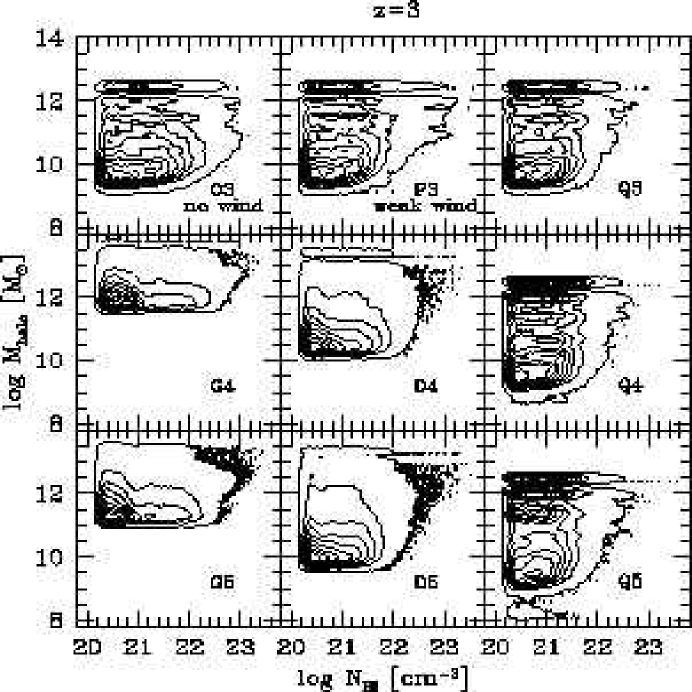
Figure 4: Hi  column density vs. dark matter halo mass at $z=3$. Each point in the figure represents one line-of-sight. Contours are equally spaced on a logarithmic scale and the lowest contour contains 95% of all the points. The highest resolution run in this figure is Q5 (bottom left panel).

In Figure 4, we show the Hi  column density of DLA sight-lines against the dark matter halo mass in which DLAs reside. The calculation of the Hi  column density is carried out exactly the same way as we did in Nagamine, Springel, & Hernquist (2003), which we summarise briefly here. First, we identify dark matter haloes by applying a conventional friends-of-friends algorithm to the dark matter particles in each simulation. After dark matter haloes are identified, we associate each gas and star particle with their nearest dark matter particle, including them in the particle list of the corresponding haloes, when appropriate. Then, for each halo, a uniform grid covering the entire halo, with grid-size equal to the gravitational softening length, is placed at the centre-of-mass of the halo. The neutral mass of each gas particle is smoothed over a spherical region of grid-cells, weighted by the SPH kernel. We then project the neutral gas in the halo onto a plane, and obtain the column density of each grid-cell in this plane.

We regard each grid-cell on the $xy$-plane as one sight-line, as we have no power to resolve smaller scales than the gravitational softening length of each simulation. Each point in the figure represents one sight-line. Contours are in equal logarithmic scale, and the lowest contour contains 95% of all the points.

A feature to note here is that a wide range of ${\rm N_{{\rm HI}}}$ values correspond to massive haloes at $z=3$. This means that the massive haloes that host LBGs at $z=3$ also host a wide variety of DLAs. Note that, since we identified the dark matter haloes with a simple friends-of-friends algorithm, subhaloes in massive haloes are not separated from the parent halo in this figure. There is also a weak trend that less massive haloes in general host lower ${\rm N_{{\rm HI}}}$ systems, which is naturally expected. Low mass haloes with $M_{\rm halo}\leq 10^{9}\rm M_{\odot}$ tend to host only one DLA with lower ${\rm N_{{\rm HI}}}$ at the centre of the halo.

5 Projected stellar mass density and DLAs

5.1 Redshift $z=3$

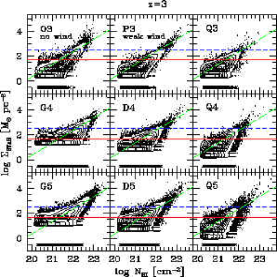
Figure 5: Projected stellar mass density vs. Hi  column density at $z=3$ (both in proper units, not comoving; same for the rest of the figures). Each point in the figure represents one line-of-sight. Contours are equally spaced on a logarithmic scale and the lowest contour contains 95% of all the points. The highest resolution run in this figure is Q5 (bottom left panel). The long-dashed line indicates the relation of the projected star-to-gas mass ratio $\Sigma_{\rm STAR}/m_{\rm p}{\rm N_{{\rm HI}}}=3$. See text for a discussion of the other 2 horizontal lines in the figure.

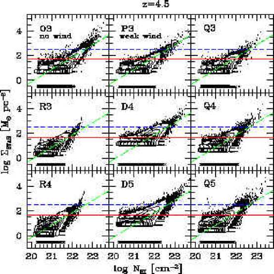
Figure 6: Projected stellar mass density vs. Hi  column density at $z=4.5$. The long-dashed line indicates the projected star-to-gas mass ratio $\Sigma_{\rm STAR}/m_{\rm p}{\rm N_{{\rm HI}}}=1$ (instead of 3 in Figure 5). The other two horizontal lines are the same as in Figure 5.

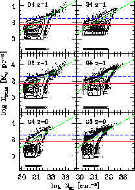
Figure 7: Projected stellar mass density vs. Hi  column density at $z=1$ and $z=0$. The long-dashed line indicates the projected star-to-gas mass ratio $\Sigma_{\rm STAR}/m_{\rm p}{\rm N_{{\rm HI}}}=10$ at $z=1$ (top 4 panels), and 20 at $z=0$ (bottom 2 panels). The other two horizontal lines are the same as in Figure 5.

In Figure 5, we show the distribution of projected stellar mass density (in proper units) of DLAs as a function of Hi  column density. Each point in the figure represents one line-of-sight. Contours are in equal logarithmic scale, and the lowest contour contains 95% of all the points. Sight-lines with no stars are shown as crosses at the bottom of each panel. As a reference, the solid horizontal line indicates an estimate of surface mass density of stars in the Milky Way, $\Sigma_{\rm STAR}=50~{}\rm M_{\odot}{\rm pc}^{-2}$, although this number is highly uncertain because of the difficulty in constraining the contribution of dark matter in the disc (Bahcall, 1984; Kuijken & Gilmore, 1989, 1991; Bahcall, Flynn, & Gould, 1992; Flynn & Fuchs, 1994; Binney & Merrifield, 1998). Most recent studies using the Hipparcos satellite data suggest that there is no compelling evidence for significant amounts of dark matter in the disc (Crézé et al., 1998; Holmberg & Flynn, 2000). The short-dashed horizontal line indicates a reference value for $\Sigma_{\rm STAR}$ if stars of total mass $10^{11}\rm M_{\odot}$ are distributed in a circle of radius 10 kpc. As a reference, we show the projected star-to-gas mass ratio of $\Sigma_{\rm STAR}/m_{\rm p}{\rm N_{{\rm HI}}}=3$ with the long-dashed line, where $m_{\rm p}$ is the proton mass. The points are distributed on both sides of this line at $20<\log{\rm N_{{\rm HI}}}<22.5$, but they preferentially lie above this line at $\log{\rm N_{{\rm HI}}}>22.5$ in all of the panels, suggesting efficient star formation at these high column densities. Stripes seen at low values of $\Sigma_{\rm STAR}$ show the discreteness due to the limited stellar mass resolution of stars in the simulation.

Comparing the top 3 panels of Figure 5, ‘O3’ (no wind), ‘P3’ (weak wind), and ‘Q3’ (strong wind), gives us an idea about the effect of the feedback by galactic winds. The runs with no winds (O3) and weak winds (P3) contain more sight-lines with high $\Sigma_{\rm STAR}$ when compared to ‘Q3’ (strong wind run, upper right corner of the panel). This is because the gas in ‘O3’ can cool and form stars continuously without being blown out by galactic winds.

As we increase the numerical resolution from Q3, Q4, and to Q5 (all strong wind runs), the number of sight-lines with $\log{\rm N_{{\rm HI}}}>22$ increases, because higher resolution runs can resolve higher gas density. Otherwise, the distribution of points in Q3, Q4, and Q5 looks similar. Comparison between D4 & D5, and G4 & G5 also shows a similar trend.

As the boxsizes become larger from the Q-Series (runs with $10h^{-1}{\rm\,Mpc}$ box) to the D- and G-series, the bottom end of the contour rises due to degrading mass resolution. A larger simulation box (G5) contains more high-mass haloes than a smaller box (Q5); therefore G5 contains more sight-lines with high $\Sigma_{\rm STAR}$ values.

5.2 Redshift $z=4.5$

In Figure 6, we show the same quantities as in Figure 5 but at redshift $z=4.5$. Horizontal solid and short-dashed lines are the same as in Figure 5. The long-dashed line here shows the projected star-to-gas ratio of $\Sigma_{\rm STAR}/m_{\rm p}{\rm N_{{\rm HI}}}=1$. The star-to-gas mass ratio at $z=4.5$ is lower than that at $z=3$ by about a factor of a few.

The highest resolution run in this figure is R4 (bottom right panel), but the boxsize of this run is small ($3.375h^{-1}{\rm\,Mpc}$). A more reliable distribution can be observed in the Q5 run.

5.3 Lower redshift

In Figure 7, we show the same quantities as in Figure 5 but at redshifts $z=1$ and $z=0$. The two horizontal lines are the same as those in Figure 5. The long-dashed line indicates the projected star-to-gas mass ratio $\Sigma_{\rm STAR}/m_{\rm p}{\rm N_{{\rm HI}}}=10$ at $z=1$ (top 4 panels), and 20 at $z=0$ (bottom 2 panels).

The observational estimate of the local star-to-gas mass ratio in the Milky Way is $\Sigma_{\rm STAR}/m_{\rm p}{\rm N_{{\rm HI}}}\approx 10$. This is obtained by dividing the estimate of $\Sigma_{\rm STAR}\approx 50~{}\rm M_{\odot}{\rm pc}^{-2}$ (assuming that there is no significant contribution of dark matter in the disc) (Bahcall, 1984; Kuijken & Gilmore, 1989, 1991; Bahcall, Flynn, & Gould, 1992; Flynn & Fuchs, 1994; Binney & Merrifield, 1998; Crézé et al., 1998; Holmberg & Flynn, 2000) by the contribution from the interstellar medium, $\Sigma_{\rm ISM}\approx 5~{}\rm M_{\odot}{\rm pc}^{-2}$ (Dame, 1993). Given the uncertainties in these numbers, the values we find in the simulation are consistent with the observed range.

An interesting evolutionary feature in the distribution can be observed as a function of redshift. At $z=3$, the distribution is wide in the horizontal direction, but as the redshift decreases, the distribution becomes narrower and elongated in the vertical direction, and the points move to higher $\Sigma_{\rm STAR}$ and lower ${\rm N_{{\rm HI}}}$ values as the neutral gas is converted into stars inside the galaxies.

6 Star formation rate of DLA galaxies

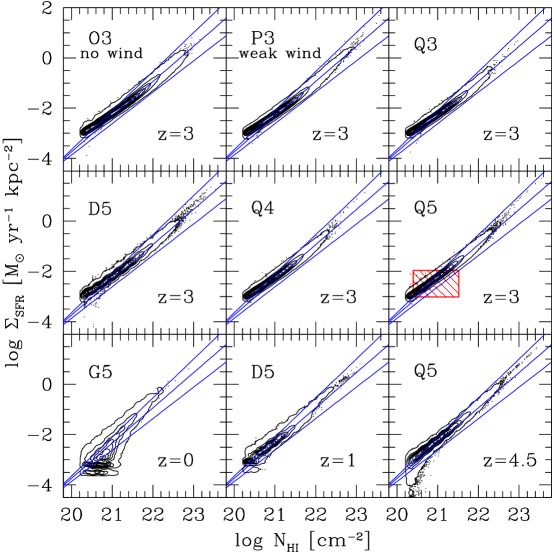
Figure 8: Projected star formation rate density vs. Hi  column density at $z=0$, 1, 3, & 4.5. Each point in the figure represents one line-of-sight. Contours are equally spaced on a logarithmic scale and the lowest contour contains 95% of all the points. The shaded region in the Q5 panel roughly indicates the region of recent observational data by Wolfe et al. (2003b).

In Figure 8, we show the projected star formation rate surface density $\Sigma_{\rm SFR}$ (in proper units of $\rm M_{\odot}\rm yr^{-1}{\rm kpc}^{-2}$) as a function of Hi  column density. The SFR of each gas particle is smoothed over a spherical region of grid-cells, weighted by the SPH kernel. This ensures that rate of star formation is conserved when added up along the $z$-direction to obtain the projected SFR density.

Each point in the figure represents one line-of-sight. Contours are equally spaced on a logarithmic scale, and the lowest contour contains 95% of all the points. The distribution was truncated at $\log{\rm N_{{\rm HI}}}=20$, so the cutoff of the contours at $\log{\rm N_{{\rm HI}}}\sim 20$ is artificial. The three solid lines in each panel show the allowed region by the following empirical relation between the projected SFR density and the Hi  column density, known as the Kennicutt law (Kennicutt, 1998):

$$\Sigma_{\rm SFR}=(2.5\pm 0.7)\times 10^{-4}\left(\frac{{\rm N_{{\rm HI}}}}{1.25\times 10^{20}\rm cm^{-2}}\right)^{1.4\pm 0.15}$$ (14)

$$\rm M_{\odot}\rm yr^{-1}{\rm kpc}^{-2}.$$ (15)

The projected SFR of DLAs in the simulation agrees well with the Kennicutt law. It may at first be surprising that the simulated result at $z=3$ follows the Kennicutt law so well, which empirically is only established for $z=0$. We will discuss this point further in Section 9. There is a slight trend in all panels for the distribution to deviate to higher values of $\Sigma_{\rm SFR}$ at $20<\log{\rm N_{{\rm HI}}}<21$ relative to the Kennicutt law, but the reason for this deviation is not clear.

The shaded area in the panel of Q5 in Figure 8 roughly indicates the region of recent observational data by Wolfe, Prochaska, & Gawiser (2003b). Their data points are close to the simulated result and roughly falls on the Kennicutt law, but the individual measurements do not with some scatter. Wolfe et al. (2003b) argue that this scatter is not surprising because their measurement of projected SFR is an average over a scale of a couple of ${\rm kpc}$ over which ${\rm N_{{\rm HI}}}$ is expected to fluctuate.

As the wind strength increases from O3 to Q3, the number of high ${\rm N_{{\rm HI}}}$ points decreases for the same reason described in Section 5.1, but otherwise the distribution remains very similar for different wind models. This is because even though the Hi  content of galaxies can be changed by a galactic wind, the star formation recipe in the code gives the same SFR for a given Hi  content. Varying the wind strength therefore only moves the points along the Kennicutt law.

Increasing the numerical resolution from Q3, Q4, and then to Q5, slightly increases the number of sight-lines at high ${\rm N_{{\rm HI}}}$ values, but the distribution is basically identical. In the G-series, one sees a sprinkle of points that fall away from the Kennicutt law at around $20<\log{\rm N_{{\rm HI}}}<21$, which is perhaps due to a lack of resolution in these large boxsize runs.

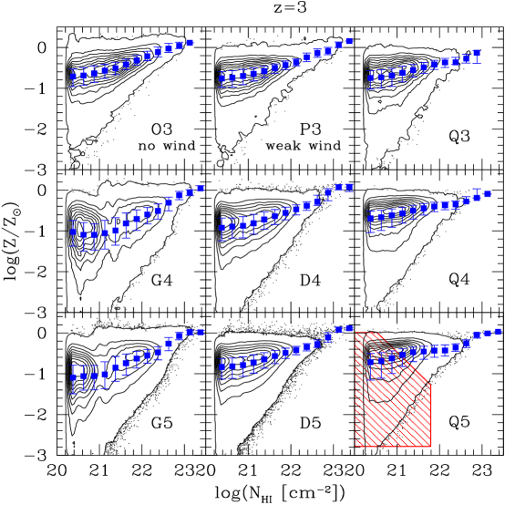
Figure 9: Gas metallicity vs. Hi  column density at $z=3$. Each point in the figure represents one line-of-sight. Contours are equally spaced on a logarithmic scale. Current observational data points fall into the shaded region that is drawn in the bottom left panel (Q5).

At $z=4.5$ (only Q5 is shown), the distribution of points seems to be tighter than that at $z=3$. An interesting feature seen at $z=4.5$ is the significant number of points falling away from the Kennicutt law at $\log{\rm N_{{\rm HI}}}\sim 20.5$. This is indicating that there are many more DLA sight-lines with inefficient star formation at $z=4.5$ compared to $z=3$, which is presumably related to the sudden decline in the DLA cross-section at around $M_{\rm halo}=10^{8.3}h^{-1}\rm M_{\odot}$, as found in Nagamine, Springel, & Hernquist (2003). At $z=4.5$, many low-mass haloes still have not accumulated enough gas for them to radiatively cool, and the neutral gas content and the SFR is significantly lower than in those at $z=3$.

At low redshift ($z=0$ & 1), the distribution starts to shrink towards lower $\Sigma_{\rm SFR}$ and lower ${\rm N_{{\rm HI}}}$ values. This can be largely understood in terms of the global evolution of the star formation efficiency in haloes, and its variation with haloes mass. As the redshift decreases, a larger fraction of the total star formation rate in the universe is contributed by ever more massive haloes (Springel & Hernquist, 2003b). In addition, at lower redshifts, haloes are less dense, and their gas has been heated by prior star formation, such that cooling becomes comparatively inefficient (Blanton et al., 1999), leading to a reduction in the star formation rates.

7 Gas Metallicity of DLAs

7.1 Redshift z=3

In Figure 9, we show the projected gas metallicity as a function of Hi  column density at $z=3$. The projected metallicity was calculated as follows: First, the metal mass and gas mass of each gas particle was smoothed over a spherical region of grid-cells, weighted by the SPH kernel. We then added up gas and metal mass independently along the $z$-direction, and finally divided the sum of the metal mass by the sum of the gas mass for each sight-line. We have also tried the same calculation by weighting with the neutral hydrogen mass instead of using the total gas mass, but the result was almost identical. We also confirmed that the result is robust even when we select out only the gas particles in high density clumps, therefore the results are not affected by the diffuse gas in the halo when projected along the $z$-direction.

Each point in the figure represents one sight-line, and the contours are equally spaced on a logarithmic scale. The solid square symbols give the median value in each $\log{\rm N_{{\rm HI}}}$ bin, with error bars indicating the quartiles on both sides. In all panels, the median metallicity increases as ${\rm N_{{\rm HI}}}$ increases, reaching solar metallicity at $\log{\rm N_{{\rm HI}}}\sim 23$. This trend is expected because star formation is more vigorous in high ${\rm N_{{\rm HI}}}$ systems, as we saw in Section 6.

In the ‘O3’ run (no wind), the contours extend to higher metallicity than in the ‘Q3’ run (strong wind). This is because in O3 star formation is not suppressed by a galactic wind. Therefore, the gas is more enriched with metals due to a higher average star formation rate. The values of the median metallicity at intermediate column densities ($20<\log{\rm N_{{\rm HI}}}<22$) are similar for all runs in the Q-series (O3, P3, Q3, Q4, and Q5).

Increasing the resolution from Q3, to Q4, and finally to Q5, increases the number of points with high metallicity at high ${\rm N_{{\rm HI}}}$ values, but otherwise the overall distribution is very similar.

It is clear that simulations with larger boxsizes, such as those of the D- and G-series, underestimate the metallicity for systems with $\log{\rm N_{{\rm HI}}}<22$ at $z=3$ due to lack of resolution. This is consistent with the finding that in the runs of the D- and G-series the Hi  column density distribution function at $z=3$ is not reliably estimated, as was shown in Nagamine, Springel, & Hernquist (2003).

An important result is that the median metallicity we find for DLAs in our simulations is much higher than the observed value. Note that observers typically find DLAs with $20<\log{\rm N_{{\rm HI}}}<22$ to have a metallicity of $Z/Z_{\odot}\sim 1/30$ (e.g. Boissé et al., 1998; Pettini et al., 1999; Prochaska & Wolfe, 2000), as indicated by the shaded region in the panel of ‘Q5’ (bottom left). We will discuss the implications of this discrepancy further in Section 9.

In Figure 10, we show the distribution of SFR as a function of metallicity at $z=3$ for the ‘Q5’-run. The recent observational data points by Wolfe, Prochaska, & Gawiser (2003b) fall into the shaded area. The shape of the simulated distribution is easy to understand: Because $\Sigma_{\rm SFR}$ is tightly correlated with ${\rm N_{{\rm HI}}}$, as we saw in Figure 8 (the Kennicutt law), the distribution seen in Figure 10 is simply a reflection of Figure 9 around a diagonal line.

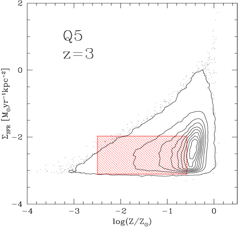
Figure 10: Projected SFR vs. gas metallicity at $z=3$ for the ‘Q5’-run. Each point in the figure represents one line-of-sight. Contours are equally spaced on a logarithmic scale. The shaded area indicates the region of observed data points by Wolfe et al. (2003b).

7.2 Redshift $z=4.5$

In Figure 11, we show the same quantities as in Figure 9, but for $z=4.5$. A noteworthy feature is that the median metallicity at $z=4.5$ is lower than that at $z=3$ by a factor of $2-3$ at column densities $\log{\rm N_{{\rm HI}}}<22$. This is consistent with the fact that the star-to-gas mass ratio at $z=4.5$ is lower than that at $z=3$ by a similar factor. The trends observed for increasing numerical resolution and wind strength are similar to those at $z=3$.

7.3 Lower redshift

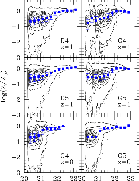
Figure 12: Gas metallicity vs. Hi  column density at $z=0$ and 1. Each point in the figure represents one line-of-sight. Contours are equally spaced on a logarithmic scale.

In Figure 12, we again analyse the same quantities as in Figure 9, but at redshifts $z=1$ and $z=0$. The most reliable of our runs at $z=1$ is ‘D5’, which shows a median metallicity that is higher by a factor of $\sim 2$ compared to that at $z=3$. A factor of 3 increase is observed for ‘G5’.

We note that the evolution in the median metallicity seen from $z=1$ to $z=0$ is quite uncertain. In fact, for the ‘G5’ run, the 3 median points at $20<\log{\rm N_{{\rm HI}}}<21$ go down by a factor of 2 from $z=1$ to $z=0$. This is because in a simulation with a large boxsize, such as ‘G5’, the mass resolution is low and many haloes are just forming at low redshift. Therefore, the number of points at $20<\log{\rm N_{{\rm HI}}}<21$ with low metallicity is still increasing from $z=1$ to $z=0$, as evidenced by the broadening of the contours towards lower metallicity. This is consistent with the fact that the value of $\Omega_{\rm HI}$ in ‘G5’ slightly increases from $z=1$ to $z=0$, as was shown in Figure 1 of Nagamine, Springel, & Hernquist (2003).

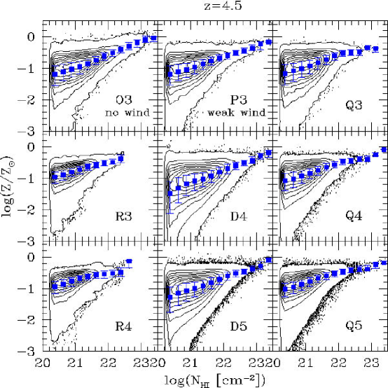
Figure 11: Gas metallicity vs. Hi  column density at $z=4.5$. Each point in the figure represents one line-of-sight. Contours are equally spaced on a logarithmic scale.

8 Mean Metallicity Evolution

In Figure 13, we compare observations of the evolution of the ${\rm N_{{\rm HI}}}$-weighted mean metallicity of DLAs with results measured from our simulations. Here, by “${\rm N_{{\rm HI}}}$-weighted”, we mean summing up all the metal mass in DLA sight-lines and dividing it by the total gas mass in all DLA sight-lines. The symbols connected by the solid lines are the direct results of our simulations for DLAs in the Q5, D5, and G5-runs. We have also tried to do the calculation in a different manner; simply taking the mean of the metallicities of all lines-of-sight in the simulations; i.e. $\left\langle Z/Z_{\odot}\right\rangle=\Sigma(Z/Z_{\odot})/N$, where $N$ is the total number of lines-of-sight. This method gives a mean metallicity which is lower by $\sim 0.1$ dex than the one obtained by the former method. This is perhaps because of the wide range of values that DLA metallicities can take, as seen in Figure 9. Our conclusion regarding the DLA metallicity does not change depending on which calculation method is used.

Column density-weighted mean observational data points by Pettini et al. (1999) (open squares) and Prochaska et al. (2003) (crosses) are also shown. Note that the error bars of Pettini et al. (1999) points are 1-$\sigma$, and those of Prochaska et al. (2003) are 95% confidence level uncertainty, both determined from a bootstrap error analysis. The long-dashed line is the best-fit line obtained by performing a least-square fit to the mean points of Prochaska et al. (2003), which exhibits a mild evolution with a slope of $-0.30$ as a function of redshift [$\log(Z/Z_{\odot})=-0.30z-0.44$]. Note that Prochaska et al. (2003) performed a least-square fit to the central values of the error bars, so they report a slope of -0.26 which is slightly different from our value, but the two agrees with each other within 1-$\sigma$.

The mean metallicity of DLAs in our simulations is again higher than current observations by about a factor of $3-5$. On the other hand, the mean metallicity of the entire simulation box (i.e. total metal mass divided by the total gas mass) is lower than the observed DLA metallicity. This makes sense because the box-mean includes low metallicity IGM that is not polluted as strongly as galaxies themselves. This simple consideration also illustrates that the metallicity values of DLAs can be quite sensitive to details of how metals are transported and mixed with gas in the haloes of galaxies and with gas in the IGM. In fact, we find that our simulations predict the correct metallicity of Lyman-$\alpha$ forest when the winds are included (Springel et al. 2003, in preparation), and that the box-mean metallicity is biased higher relative to that of the low-density IGM.

Residual differences between the results of Q5, D5, and G5 are due to numerical resolution. Higher resolution runs (like Q5) can resolve smaller haloes at high redshift than lower resolution runs (D5, G5). Therefore, Q5 has more star formation, and consequently more metal production, at high redshifts than D5 and G5.

Another noteworthy result is that the $rate$ of the evolution of mean metallicity in our simulations appears to be consistent with the most recent observed rate by Prochaska et al. (2003). In the simulation of Cen et al. (2002), a similar agreement was obtained. We will discuss this more in the following section.

9 Discussion

We have used a series of state-of-the-art hydrodynamic simulations to study the distribution of star formation rate and metallicity of DLAs. Our simulations suggest that the median projected star-to-gas mass ratio of DLAs is about a few at $z=3$, and then evolves to higher values of $\simeq 10$ at $z=1$ and $\simeq 20$ at $z=0$. However, we note that our low-redshift results should be regarded with caution because they are based on simulations with coarser resolution than those at high-redshift. Nevertheless it is encouraging that the star-to-gas mass ratio we find at $z=0$ is close to observational estimates for the Milky Way (see Section 5.3).

The projected SFR density as a function of neutral hydrogen column density follows the Kennicutt law well at all redshifts. At first sight, this may seem non-trivial and perhaps somewhat surprising. However, the star formation model adopted in the simulations depends only on local physical quantities, e.g. the local gas density. The free parameter of the model was chosen to reproduce the Kennicutt law in isolated disk galaxies at low redshift, but was kept fixed as a function of time. We hence implicitly assumed that the Kennicutt law holds at all redshifts, and our simulation results reflect this assumption.

A recent study by Kravtsov (2003) also suggests that the projected SFR follows the global ‘Schmidt’ law, and that it does not depend on redshift. He argues that the global Schmidt-law originates from a generic power-law distribution of the high-density tail of the probability distribution function of gas density. If the star formation at high-redshift follows similar physical process as in the Local Universe, it is not unreasonable that the projected SFR should follow the Kennicutt law well even at high redshift.

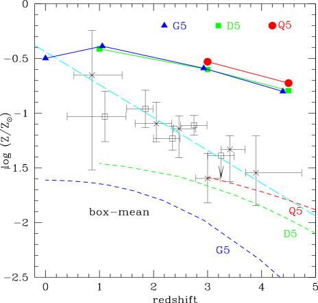
Figure 13: Evolution of the mean gas metallicity of DLAs as a function of redshift. The symbols connected by solid lines give the direct simulation results for the Q5, D5, and G5-runs. The short-dashed lines at the bottom of the figure are the mean metallicities of the entire simulation boxes. Data points with error bars show observations by Pettini et al. (1999) (open squares) and Prochaska et al. (2003) (crosses). The long-dashed line is the best-fit line obtained by performing a least-square fit to the mean points of Prochaska et al. (2003), which exhibits a mild evolution with a slope of $-0.30$ as a function of redshift.

The Hi  column density distribution in our simulations extends up to values as high as $\log{\rm N_{{\rm HI}}}\sim 23$, which is in the range of Hi  column densities seen in the nuclei of starburst galaxies in the Local Universe. This suggests that the intense star-formation seen in some of the brightest simulated galaxies at $z=3$ is similar to the star formation in local starburst galaxies. These simulated galaxies should then correspond to the observed Lyman-break galaxies, which are often estimated to have SFRs of $\sim 50-100\rm M_{\odot}\rm yr^{-1}$, or even higher. The spatial correlation between Lyman-break galaxies and DLAs is hence of significant interest to elucidate this connection further, and we will study this issue in future work.

While the star-to-gas mass ratio and the projected SFR density at $z=3$ in the simulations seems to be plausible, the median metallicity of DLAs at $z=3$ appears to be too high ($Z/Z_{\odot}\sim 1/3$) compared to typically observed values of $Z/Z_{\odot}\sim 1/30$ for DLAs (e.g. Pettini et al., 1999). There are a number of possible explanations for this problem, and we will briefly discuss some of the most prominent possibilities.

Since the SFRs and metallicities of galaxies in the simulation at $z=3$ seem plausible, one possible reason for high metallicity in DLAs is that the feedback by galactic winds is not efficient enough in blowing out metals from DLAs. Clearly, if the feedback by winds were stronger, then star formation and hence metal creation in DLAs would be more strongly suppressed. In fact, the SFR of systems with $20<\log{\rm N_{{\rm HI}}}<21$ deviates slightly from the Kennicutt law to higher values in our simulation. Reducing the SFR of these systems would bring them down to values consistent with the Kennicutt law.

However, simply making the winds stronger and blowing out more gas will not necessarily decrease the metallicity of DLAs much, because in our current simulation model, the wind transports away metals and gas at the same time, i.e. the wind’s initial metallicity is assumed to be equal to that of the gas of the DLA, leaving the ratio of metal and gas mass in the DLA unchanged.

It is however quite plausible that the wind is metal-loaded compared to the gas in the DLA, as is for example suggested by simulations of SN explosions (e.g. MacLow & Ferrara 1999, Bromm et al. 2003). After all, the ejecta of SN are heavily enriched and inject large parts of the energy that is assumed to ultimately drive the outflow. If the mixing with other DLA-gas is not extremely efficient before the outflow occurs, it can then be expected that the wind material has potentially much higher metallicity than the DLA, thereby selectively removing metals.

A related possibility concerns the metallicities of the cold and diffuse phases of the DLA. In the present study, we assumed that metals are always efficiently and rapidly mixed between the gas of the cold clouds and the ambient medium, such that there is a homogeneous metal distribution in the DLA (operationally, we used only a single metallicity variable for each gas particle, reflecting this assumption). However, this assumption may not be fully correct. If the metals were preferentially kept in the hot phase of the ISM after they are released by SN, then they would not be observed in the cold gas that is responsible for the DLAs. Since we did not track the metal distribution in cold and hot phases separately in the current simulations, we may then have overestimated the amount of metals in DLAs by counting those in the hot phase as well as those in the cold phase. Note that a more detailed tracking of metals in the simulation, separately for hot and cold phases of the gas, could in principle be done easily on a technical level. The difficulty however lies in obtaining a reasonable description of the physics that governs the exchange of metals between the different phases of the ISM, something that is presently not attainable from either observation or theory.

The viability of the feedback model in the simulations can also be tested by comparing with observations of the Lyman-$\alpha$ forest, which is generated by systems of much lower column density than the DLAs studied in this work. Curiously, an analysis using the current simulation series (Springel et al. 2003, in preparation), as well as a study by Theuns et al. (2002), suggest that the spectral features of the Ly-$\alpha$ forest are not significantly affected by the feedback from galactic outflows, despite the fact that the wind strength is taken to be on the ‘strong side’ in these studies, and despite the fact that a non-negligible fraction of the IGM volume is heated by the winds. Note that in our simulations with a strong wind model, the Hi  mass density in the entire simulation box is somewhat lower than suggested by observational estimates (Nagamine, Springel, & Hernquist, 2003), therefore it appears problematic to increase the wind strength even beyond the present value.

The high metallicity of DLAs may also be related to the steep luminosity function of galaxies in our SPH simulations. A preliminary analysis using a population synthesis model shows that the luminosity function still has a very steep slope at the faint end even at low redshift, similar to that of the dark matter halo mass function. (It is not obvious whether the steep faint end in the simulation at $z>1$ is a problem, because it is not well constrained observationally at $z>1$ yet.) This means that the formation of low-mass galaxies in our simulation was not suppressed enough, or equivalently, that star formation was too efficient in low-mass haloes. Stronger winds may help to alleviate this problem, but it appears unlikely that our present feedback model can solve it satisfactorily simply by adopting a higher efficiency parameter for feedback. It is more plausible that additional physical processes need to be considered in a more faithful way. One simple possibility for this is related to the UV background field, which is turned on by hand at $z=6$ in our present simulations to mimic reionisation of the Universe at a time when the first Gunn-Peterson troughs in spectra to distant quasars are observed (Becker et al., 2001). However, it is possible (in fact suggested by the WMAP satellite) that the Universe was reionised at much higher redshift. The associated photoheating may have then much more efficiently impaired the formation of low-mass galaxies than in our present simulations (but see Dijkstra et al., 2003). We plan to explore this possibility in future work by adopting different treatments of the UV background radiation field.

It is also interesting to compare our results with other hydrodynamic simulations of DLAs. Cen et al. (2002) have recently studied the metallicity of DLAs in an Eulerian hydrodynamic simulation of boxsize ${\rm L_{box}}=25h^{-1}{\rm\,Mpc}$. The median metallicity as a function of Hi  column density in their simulation is lower than ours by a factor of $\sim 5$, in better agreement with observations (but still higher than observations by about a factor of a few). This difference between the two simulations could be due to the difference in the efficiency of the SN feedback, which in turn originates in the widely different spatial resolutions of the two simulations. The Eulerian simulation of Cen et al. used a fixed grid, where the energy and the metals released by SN were dumped into the gas of those local cells that showed star formation activity. Since the comoving cell size of their simulation was $32.6h^{-1}{\rm\,kpc}$, metals were thus distributed efficiently over this spatial scale by construction, diluting the metal mass relative to the gas mass in the cell for a given amount of stars formed. On the other hand, in our present SPH simulations, the gravitational softening length was typically only a few kpc comoving, such that the gas particles would in fact have to travel over a large number of resolution elements in order to distribute the injected metals over similar spatial scales as in the mesh simulation.

Despite the differences in the metallicity values of DLAs measured in the two simulations, there are also important common features. One of them is the existence of high ${\rm N_{{\rm HI}}}$ systems with high metallicity, which are absent in current observations. The existence of such a population of DLAs may perhaps be a generic prediction of current CDM simulations. Cen et al. (2002) invoked a dust obscuration effect in order to reconcile their result with observations, and argued that their column density distribution, Hi  mass density, and DLA-metallicity would all become consistent with observations, provided a sizable dust extinction is assumed. However, it is presently not very clear how strong dust effects really are (e.g. Ellison et al., 2001; Prochaska & Wolfe, 2002), and the solution could rather lie in a more adequate treatment of star formation and supernova feedback, as Cen et al. (2002) also warn. For example, Schaye (2001) argues that the conversion of neutral hydrogen atoms into a molecular form, which we have not yet implemented in our simulations, would introduce a physical limit to the highest ${\rm N_{{\rm HI}}}$ that DLAs can attain. This process would eliminate the highest ${\rm N_{{\rm HI}}}$ systems, but would not reduce the metallicity of low ${\rm N_{{\rm HI}}}$ systems because it would make the star formation even more efficient than it is in current simulations. If future cosmological simulations with a more sophisticated modelling of star formation and SN feedback confirm the existence of high-metallicity, high-${\rm N_{{\rm HI}}}$ systems, then they could turn into an interesting challenge for the CDM model.

Another important common feature found in both simulation studies is the mild evolution of the mean metallicity of DLAs with redshift. It is encouraging that the two entirely different simulation methodologies agree on the rate of this evolution, which in turn is consistent with the observed rate. Note that processes such as galaxy mergers, gas infall, and outflows all play an important role in the chemical evolution of DLAs, and these processes, which often cannot be treated accurately in semi-analytic models of the chemical evolution of DLAs, are included dynamically and self-consistently in both simulations.

In conclusion, together with our previous results presented in Nagamine, Springel, & Hernquist (2003), we have shown that the DLAs found in our simulation series have many plausible properties. In particular, they are in good agreement with recent observations of the total neutral Hi  mass density, the Hi  column density distribution function, the abundance of DLAs, and the distribution of SFR in DLAs. However, our simulated DLAs show typically considerably higher metallicity than what is presently observed for the bulk of these systems. This likely indicates that metal transport and mixing processes have not been efficient enough in our simulations. It will be interesting to study more sophisticated metal enrichment models in future simulations in order to further improve our understanding of the nature of DLAs in hierarchical CDM models.

References

- Adelberger et al. (1998) Adelberger K. L., Steidel C. C., Giavalisco M., Dickinson M., Pettini M., Kellogg M., 1998, ApJ, 505, 18
- Bahcall (1984) Bahcall J. N., 1984, ApJ, 287, 926
- Bahcall, Flynn, & Gould (1992) Bahcall J. N., Flynn C., Gould A., 1992, ApJ, 389, 234
- Baugh et al. (1998) Baugh C. M., Cole S., Frenk C. S., Lacey C. G., 1998, ApJ, 498, 504
- Becker et al. (2001) Becker R. H., et al. 2001, AJ, 122, 2850
- Binney & Merrifield (1998) Binney J., Merrifield M., 1998, Galactic Astronomy, Princeton University Press, p.656-664
- Blain et al. (1999) Blain A. W., Smail I., Ivison R. J., Kneib J.-P., 1999, MNRAS, 302, 632
- Blanton et al. (1999) Blanton M., Cen R., Ostriker J. P., Strauss M. A., 1999, ApJ, 522, 590
- Boissé et al. (1998) Boissé P., Le Brun V., Bergeron J., Deharveng J. M., 1998, A&A, 333, 841
- Bromm et al. (2003) Bromm V., Yoshida N., Hernquist L., 2003, ApJ, submitted. (astro-ph/0305333)
- Cen et al. (2002) Cen R., Ostriker J. P., Prochaska J. X., Wolfe A. M., 2002, preprint (astro-ph/0203524)
- Crézé et al. (1998) Crézé M., Chereul E., Bienaymé O., Pichon C., 1998, A&A, 329, 920
- Croft et al. (2001) Croft R. A. C., Di Matteo T., Davé R., Hernquist L., Katz N., Fardal M. A., Weinberg D.H., 2001, ApJ, 557, 67
- Dame (1993) Dame T. M., 1993, Back to the Galaxy, AIP Conference Proceedings 278, eds. Holt, S. S., Verter, F. (New York: AIP), p.267
- Davé et al. (1999) Davé R., Hernquist L., Katz N., Weinberg D. H., 1999, ApJ, 511, 521
- Dijkstra et al. (2003) Dijkstra M., Haiman Z., Rees M. J., & Weinberg D. H. 2003 (astro-ph/0308042)
- Ellison et al. (2001) Ellison S. L., Yan L., Hook I. M., Pettini M., Wall J. V., Shaver P. 2001, A&A, 379, 393
- Flynn & Fuchs (1994) Flynn C., Fuchs B., 1994, MNRAS, 270, 471
- Gardner et al. (1997a) Gardner J. P., Katz N., Hernquist L., Weinberg D. H., 1997a, ApJ, 484, 31
- Gardner et al. (1997b) Gardner J. P., Katz N., Weinberg D. H., Hernquist L., 1997b, ApJ, 486, 42
- Gardner et al. (2001) Gardner J. P., Katz N., Hernquist L., Weinberg D. H., 2001, ApJ, 559, 131
- Haardt & Madau (1996) Haardt F., Madau P., 1996, ApJ, 461, 20
- Hernquist (1993) Hernquist L., 1993, ApJ, 404, 717
- Hernquist & Springel (2003) Hernquist L., Springel V., 2003, MNRAS, 341, 1253
- Holmberg & Flynn (2000) Holmberg J., Flynn C., 2000, MNRAS, 313, 209
- Jimenez et al. (1999) Jimenez R., Bowen D. V., Matteucci F., 1999, ApJ, 514, L83
- Katz, Hernquist & Weinberg (1999) Katz N., Hernquist L., Weinberg D. H., 1999, ApJ, 523, 463
- Katz et al. (1996) Katz N., Weinberg D. H., Hernquist L., 1996, ApJS, 105, 19
- Kauffmann (1996) Kauffmann G., 1996, MNRAS, 281, 475
- Kauffmann et al. (1999) Kauffmann G. A. M., Colberg J. M., Diaferio A., White S. D. M., 1999, MNRAS, 307, 529
- Kennicutt (1998) Kennicutt, R. C. Jr., 1998, ARA&A, 36, 189
- Kravtsov (2003) Kravtsov A. V. 2003, preprint (astro-ph/0303240)
- Kuijken & Gilmore (1991) Kuijken K., Gilmore G., 1991, ApJ, 367, L9
- Kuijken & Gilmore (1989) Kuijken K., Gilmore G., 1989, MNRAS, 239, 605
- Laird et al. (1988) Laird J. B., Rupen M. P., Carney B. W., Latham D. W. 1988, AJ, 96, 1908
- Lanfranchi & Friaca (2003) Lanfranchi G. A., Friaca A. C. S., 2003, MNRAS, in press (astro-ph/0304119)
- Lanzetta et al. (2002) Lanzetta K. M., Yahata N., Pascarelle S., Chen H-W., Fernández-Soto A., 2002, ApJ, 570, 492
- Lanzetta (1993) Lanzetta K. M. 1993, in The Environment and Evolution of Galaxies, eds. J. M. Shull & H. A. Thronson (Dordrecht: Kluwer), p237
- Lu et al. (1996) Lu L, Sargent W. L. W., Barlow T. A., Churchill C. W., Vogt S., 1996, ApJS, 107, 475
- Lucy (1977) Lucy L., 1977, AJ, 82, 1013
- Mac Low & Ferrara (1999) Mac Low, M. M. & Ferrara, A., 1999, ApJ, 513, 142
- Maller, Prochaska, Somerville, & Primack (2002) Maller A. H., Prochaska J. X., Somerville R. S., Primack J. R., 2002, MNRAS, submitted (astro-ph/0211231)
- Maller, Prochaska, Somerville, & Primack (2001) Maller A. H., Prochaska J. X., Somerville R. S., Primack J. R., 2001, MNRAS, 326, 1475
- McKee & Ostriker (1977) McKee C. F., Ostriker, J. P., 1977, ApJ, 218, 148
- Mo, Mao, & White (1999) Mo H. J., Mao S., White S. D. M., 1999, MNRAS, 304, 175
- Mo & Fukugita (1996) Mo H. J., Fukugita, 1996, ApJ, 467, L9
- Nagamine, Springel, & Hernquist (2003) Nagamine K., Springel V., Hernquist L., 2003, MNRAS, submitted (astro-ph/0302187)
- Nagamine (2002) Nagamine K., 2002, ApJ, 564, 73
- Nagamine et al. (2001) Nagamine K., Fukugita M., Cen R., Ostriker J. P., 2001, ApJ, 558, 497
- Pascarelle, Lanzetta, & Fernández-Soto (1998) Pascarelle S., Lanzetta K. M., Fernández-Soto A., 1998, ApJ, 508, L1
- Pearce et al. (1999) Pearce et al., 1999, ApJ, 521, 99
- Pei & Fall (1995) Pei Y. C. & Fall S. M. 1995, ApJ, 454, 69
- Pettini (2003) Pettini M. 2003, XIII Canary Islands Winter School of Astrophysics, ‘Cosmochemistry: The Melting Pot of Elements’ (astro-ph/0303272)
- Pettini et al. (1999) Pettini M., Ellison S. L., Steidel C. C., Bowen D. V. 1999, ApJ, 510, 576
- Pettini et al. (1994) Pettini M., Smith L. J., Hunstead, R. W., King D. L., 1994, ApJ, 426, 79
- Prantzos & Boissier (2000) Prantzos N., Boissier S., 2000, MNRAS, 315, 82
- Prochaska et al. (2003) Prochaska J. X., Gawiser E., Wolfe A. M., Castro S., Djorgovski G., 2003, ApJ, submitted (astro-ph/0305314)
- Prochaska & Wolfe (2002) Prochaska J. X. & Wolfe A. M., 2002, ApJ, 566, 68
- Prochaska & Wolfe (2000) Prochaska J. X. & Wolfe A. M., 2000, ApJ, 533, L5
- Prochaska & Wolfe (1999) Prochaska J. X. & Wolfe A. M., 1999, ApJS, 121, 369
- Prochaska & Wolfe (1998) Prochaska J. X. & Wolfe A. M., 1998, ApJ, 507, 113
- Schaye (2001) Schaye, J. 2001, ApJ, 562, L95
- Shapley et al. (2001) Shapley A. E., Steidel C. C., Adelberger K. L., Dickinson M., Giavalisco M., Pettini M., 2001, ApJ, 562, 95
- Sokasian et al. (2003) Sokasian A., Abel T., Hernquist L., Springel V., 2003, MNRAS, in press (astro-ph/0303098)
- Somerville, Primack, & Faber (2001) Somerville R. S., Primack J. R., Faber S. M., 2001, MNRAS, 320, 504
- Springel & Hernquist (2002) Springel V., Hernquist L., 2002, MNRAS, 333, 649
- Springel & Hernquist (2003a) Springel V., Hernquist L., 2003a, MNRAS, 339, 289
- Springel & Hernquist (2003b) Springel V., Hernquist L., 2003b, MNRAS, 339, 312
- Springel, Yoshida & White (2001) Springel V., Yoshida N., White S. D. M., 2001, New Astronomy, 6, 79
- Steidel et al. (1999) Steidel C. C., Adelberger K. L., Giavalisco M., Dickinson M., Pettini M., 1999, ApJ, 519, 1
- Storrie-Lombardi & Wolfe (2000) Storrie-Lombardi L. J., Wolfe A. M., 2000, ApJ, 543, 552
- Theuns et al. (2002) Theuns T., Viel M., Kay S., Schaye J., Carswell R. F., Tzanavaris P. 2002, ApJ, 578, L5
- Wolfe, Prochaska, & Gawiser (2003a) Wolfe A. M., Prochaska J. X., Gawiser E., 2003a, ApJ, in press (astro-ph/0304040)
- Wolfe, Prochaska, & Gawiser (2003b) Wolfe A. M., Prochaska J. X., Gawiser E., 2003b, preprint (astro-ph/0304042)
- Wolfe et al. (1995) Wolfe A. M., Lanzetta K. M., Foltz C. B., 1995, ApJ, 454, 698
- Wolfe et al. (1986) Wolfe A. M., Turnshek D. A., Smith H. E., Cohen R. S., 1986, ApJS, 61, 249
- Weinberg, Hernquist, & Katz (2002) Weinberg D. H., Hernquist L., Katz N., 2002, ApJ, 571, 15
- Yoshida et al. (2002) Yoshida N, Stoehr F., Springel V., White S. D. M., 2002, MNRAS, 335, 762
- Wyse & Gilmore (1995) Wyse R. F. G. & Gilmore G. 1995, AJ, 110, 2771