Some aspects of Relativistic Astrometry from within the Solar System

Abstract

In this article we outline the structure of a general relativistic astrometric model which has been developed to deduce the position and proper motion of stars from 1-microarcsecond optical observations made by an astrometric satellite orbiting around the Sun. The basic assumption of our model is that the Solar System is the only source of gravity, hence we show how we modeled the satellite observations in a many-body perturbative approach limiting ourselves to the order of accuracy of $(v/c)^{2}$. The microarcsecond observing scenario outlined is that for the GAIA astrometric mission.

Appl. Opt.
Maria Teresa Crosta
INAF - Osservatorio Astronomico di Torino
strada Osservatorio 20
10025 Pino Torinese (TO)
Italy

GR General Theory of Relativity; CM Center of Mass

1 Introduction

Aim of fundamental astrometry is to measure stellar positions, parallaxes and proper motion directly from optical observations. Understanding how electromagnetic waves propagate in a time dependent gravitational field is essential to answer basic questions in astrophysics. In fact, most of the physical information about the surrounding universe (see 1999PhRvD..59h4023K, 2001ApJ…556L…1K and references therein) is carried by light signals. Nowadays the scientific objectives of astrometry and astrophysics can be combined thanks to the precision achievable by the new generation of space astrometry missions like GAIA of the European Space Agency (ESA). GAIA will be launched not later then 2012 (with a possible window in 2010) and is expected to make astrometric measurements with a precision of a few $\mu$arcsec [Perryman et al. (2001)]. At this level of accuracy one should consider contributions to the light deflection not only by the mass of the Sun and of the other planets, but also by their gravitational quadrupole moments as well as their translational and rotational motion (table 1). This implies that a suitable reduction of the GAIA observational data requires the development of a model of the celestial sphere more sophisticated than the one used for Hipparcos, the first global astrometry satellite launched by ESA in 1989. All mathematical and physical assumptions which characterize our model, as we shall specify in sections 2 and 3, are tailored to the GAIA concept.

	$\delta\chi_{\textrm{pN}}$		$\delta\chi_{J_{2}}$		$\delta\chi_{L}$		$\chi_{\textrm{max}}$
Sun	$1.\!\!^{\prime\prime}75$		$\sim 1$	$\mu$as	0.7	$\mu$as	$(180^{\circ})$
Mercury	$83$	$\mu$as	–		–		$(7^{\prime})$
Venus	$493$		–		–		$(4.0^{\circ})$
Earth	$574$		$0.6$		–		$(101^{\circ})$
Moon	$26$		–		–		$(2.3^{\circ})$
Mars	$116$		$0.2$		–		$(17^{\prime})$
Jupiter	$16290$		$240$		$0.2$		$(87^{\circ}/3^{\prime})$
Saturn	$5772$		$94$		–		$(16^{\circ}/51^{\prime\prime})$
Uranus	$2030$		$7$		–		$(67^{\prime}/4^{\prime\prime})$
Neptune	$2487$		$8$		–		$(50^{\prime}/3^{\prime\prime})$
Pluto	$7$		–		–		$(0^{\prime\prime}\!\!.3)$
Io	$30$		–		–		$(18^{\prime\prime})$
Europe	$19$		–		–		$(10^{\prime\prime})$
Ganymede	$34$		–		–		$(30^{\prime\prime})$
Callisto	$27$		–		–		$(22^{\prime\prime})$

Table 1: Detectable first order post-Newtonian relativistic effects in Solar System at 1 $\mu$arcsec level. Here $\delta\chi_{\mathrm{pN}}$ is the contribution due to the spherically symmetric component of the gravitational field of the corresponding body, $J_{2}$ is that of the quadrupolar moment, and $L$ that of the rotational motion. The values whitin the parenthesis represents the maximum angular distance between the perturbing body and photon at which the effect still attains 1 $\mu$arcsec; where two values are reported, they refer to the pN and the $J_{2}$ cases respectively. The pN values have been calculated considering an observer at L2 in the Sun-Earth system, and using the data reported in 1999ssd.book…..M for the Solar System bodies.

GAIA’s main scientific objective is to shed definitive light on the origin, structure and kinematics of the Galaxy utilizing a complete census of the entire sky down to the visual magnitude $V=20$, for a total of about one billion stars. This survey is achieved by exploiting the same scanning strategy which was used with the successful astrometric mission Hipparcos. In this way GAIA will measure the effects of many thousands of extra solar planets, and determine their orbit; thousands of brown dwarf and white dwarfs will also be identified. Many thousands of new minor bodies, inner Trojans, and even new Trans-Neptune objects, including Plutinos, may be discovered. The main physical properties of asteroids ($10^{5}-10^{6}$ new objects) will be investigated including masses, densities, sizes, shapes and taxonomic classes. In particular, asteroid mass is determined by measuring the tiny gravitational perturbations experienced in case of mutual close approaches [Bienaymé and Turon (2002)].

Moreover GAIA’s $\mu$arcsecond global astrometry allows one to test General Relativity (GR). Realistic end-to-end simulations in fact [Vecchiato et al. (2003)] show that GAIA could measure the PPN parameter $\gamma$ to $\sim 10^{-7}$ (1$\sigma$) after 5 years of continuous observations. The parameter $\gamma$ measures the excess of curvature produced by mass-energy as compared to GR where its value is 1. As well known (1993PhRvL..70.2217D; Damour et al. 2002a; 2002b) a deviation from $\gamma$’s GR value would deeply affect our understanding of fundamental physics.

In what follows, greek indices run from 0 to 3 and latin indices run from 1 to 3.

2 Modeling the observations of GAIA

The astrometric problem consists in the determination, from a prescribed set of observables, of the astrometric parameters of a star namely its coordinates, parallax and proper motion. While in classical astrometry these quantities are well defined, in GR they must be interpreted consistently with the relativistic framework of the model.

The first step of the modeling is to identify the gravitational sources and then fix the background geometry. Next we choose a suitable reference system to label space-time points and describe the light trajectory, the stellar motion and the motion of the observer. Evidently the goal of our model is to write a formula which relates the observables to the astrometric parameters. To this purpose we had to take into account the way how the satellite GAIA will operate.

Our first assumption is that the Solar System is the only source of gravity; in doing so we ignore, e.g., microlensing effects which are perhaps the most important perturbations suffered by a light ray in its way to us since they generate systematic errors in the data reduction. However, their expected number is very small as compared to the number of stars surveyed by GAIA ($\geq 10^{9}$) hence we feel justified neglecting them at least at this stage of modeling.

The second assumption is to consider the Solar System as a source of a weak gravitational field. This allows us to adopt a quasi-Minkowskian metric

$$g_{\alpha\beta}=\eta_{\alpha\beta}+h_{\alpha\beta}+O(h^{2})$$ (1)

where the $h_{\alpha\beta}$ are perturbation coefficients such that $|h_{\alpha\beta}|\ll 1$; their spatial variations are at most of the order of $|h_{\alpha\beta}|$ while their time variations are at most of the order of $(v/c)|h_{\alpha\beta}|$ where $c$ is the velocity of light in vacuum and $v$ is the typical velocity within the perturbing system. Notice that $v$ represents the velocity needed to be gravitationally bounded in the Solar System Damour (1987), and its typical value for the energy balance (virial theorem) is $\sim 10~{}\textrm{km}\,\textrm{s}^{-1}$. Under these conditions we shall take $h_{\alpha\beta}=\sum_{a}h^{(a)}_{\alpha\beta}$ where the sum is extended to the bodies of the Solar System. The order of magnitude of each term $h^{(a)}_{\alpha\beta}$ can be expressed in term of powers of $(v/c)$. Since the $h$ terms are at least of order $(v/c)^{2}$, the level of accuracy which is expected to be reached within the model is fixed by the order of $(v/c)$ to which one likes to extend the calculation. Having these considerations in mind, we shall adopt the IAU recommended metric form for the barycentric reference frame inside the Solar System IAU (2000). In this case the lowest orders of magnitude of the metric coefficients are $h_{00}=O((v/c)^{2})$, $h_{ij}=O((v/c)^{2})$ and $h_{0i}=O((v/c)^{3})$. In the following we describe the construction of a model accurate to $(v/c)^{2}$ where in addition we approximate the Solar System to a static, non-rotating and non-expanding gravitating system and therefore we do not need to consider the spatial location of the individual gravitational sources at the corresponding retarded time. This assumption implies that in reconstructing the light trajectory of each photon emitted by a distant star, we keep the bodies of the Solar System fixed at the position they have with respect to its center of mass (CM) at the time of observation, say. Evidently each subsequent light ray will be reconstructed updating the positions of the bodies of the Solar System according to their actual motion. This does not mean that the bodies are at rest in the model, but that in our $(v/c)^{2}$ approximation their position can be considered fixed in a single integration. This model will serve as a touchstone for comparison once we extend our analysis to the order of $(v/c)^{3}$.

Let $(\tau,x,y,z)$ be a coordinate system with respect to which the spacetime metric takes the form (1). Up to the order $(v/c)^{2}$ the space-time certainly admits a vorticity free congruence of curves which allows for a spacetime foliation into three dimensional hypersurfaces with equation $\tau=$constant; we shall term them $S(\tau)$ and identify the normals with a unitary vector field $u^{\alpha}=dx^{\alpha}/d\sigma$ with $x^{\alpha}\equiv{\tau,x,y,z}$ as $\alpha=0,1,2,3$. In this case the spatial coordinates can be fixed within each slice up to spatial transformations only. We can then give the vector field $u^{\alpha}$ the form $u^{\alpha}=(-g_{00})^{-1/2}\delta^{\alpha}_{\tau}$ which makes the vector unitary. The vector field so defined describes a physical observer with proper time $\sigma$ who Lie-transports the spatial coordinates. We also require that the CM of the Solar System (figure 1) and the planets belong to this congruence. At this point of the modeling we have characterized the metric, the coordinate system and a physical observer $u$$u$$u$ who is at rest with respect to the CM of the Solar System and therefore termed baricentric; we can now trace the light path.

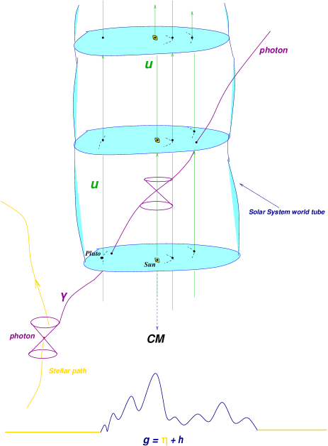
Figure 1: The astronomical set-up. A photon crosses the Solar System which is the only source of gravity. The vector field $u$$u$$u$ describes physical observers who Lie-transports the spatial coordinates (including those of the planets at the $(v/c)^{2}$ order).

Let $\mit\Upsilon$ be a null geodesic with tangent vector field $k^{\alpha}\equiv d\xi^{\alpha}/d\lambda$ (here $\lambda$ is a real parameter on $\mit\Upsilon$). A photon traveling from a distant star to the astrometric satellite within the Solar System would see the spacetime as a time development of the spatial hypersurfaces $S(\tau)$. The light trajectory will end at the satellite at a coordinate time $\tau_{0}$ and at a point with spatial coordinates $x^{i}_{o}$. Because the spacetime is foliated into slices $S(\tau)$ each representing a surface of simultaneity for the baricentric observer $u$$u$$u$ namely her/his rest space, each point $\mit\Upsilon(\lambda)$ on the null geodesic can be mapped into the point on the slice $S(\tau_{0})$ where the unique normal to $S(\tau)$ at $\mit\Upsilon(\lambda)$ crosses $S(\tau_{0})$, (see figure 2). In doing so the entire curve $\mit\Upsilon$ is mapped into a curve $\bar{\mit\Upsilon}$ in $S(\tau_{0})$; this curve has a tangent vector $\ell^{\alpha}$ which at every point of $\bar{\mit\Upsilon}$ is numerically equal to the components of the null vector $k^{\alpha}$ in the rest space of $u$$u$$u$ at the corresponding point of $\mit\Upsilon(\lambda)$.

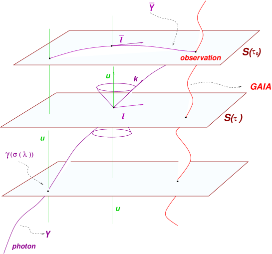
Figure 2: Mapping the null ray into the rest space of the barycentric observer in the case of a model accurate at the $(v/c)^{2}$ order.

Neglecting the time variations of the metric and imposing $h_{0i}=0$ the geodesic equation for the light ray leads, after some algebra, to the differential equations of $\bar{\mit\Upsilon}$. For the corresponding tangent field $\ell$$\ell$$\ell$ these differential equations read:

$$\frac{d\bar{\ell}^{k}}{d\sigma}+\bar{\ell}^{k}\left(\frac{1}{2}\bar{\ell}^{i}\partial_{i}h_{00}\right)+\left(\partial_{i}h_{kj}-\frac{1}{2}\partial_{k}h_{ij}\right)\bar{\ell}^{i}\bar{\ell}^{j}-\frac{1}{2}\partial_{k}h_{00}=0,$$ (2)

where $\bar{\ell}$$\bar{\ell}$$\bar{\ell}$ is the unitary tangent vector field obtained reparametrizing the tangent field $\ell$$\ell$$\ell$, which is in general not unitary, and $\delta^{ks}$ is the Kronecker delta.

To integrate equation (2) one needs to fix boundary conditions; these will be given by the components $\bar{\ell}^{i}_{0}$ of the vector field $\bar{\ell}$ at the observation point, namely at $\tau=\tau_{0}$ and $x^{i}=x^{i}_{0}$. When the light ray is intercepted by the satellite then the angles between the direction of the incoming photon as seen by an observer comoving with the satellite and the three spatial directions of a triad adapted to that observer, will be the observables. These are essential to fix the required boundary conditions namely to express the components $\bar{\ell}^{i}_{0}$ in terms of known quantities alone. Our task now is to solve this problem.

Let ${\bf u^{\prime}}$ be the unitary vector field tangent to the satellite’s world line and let {${\kern-0.24994pt\hbox{$\lambda$}\kern-5.83336pt\kern 0.50003pt\hbox{$\lambda$}\kern-5.83336pt\kern-0.24994pt\raise 0.43304pt\hbox{$\lambda$}_{\hat{a}}}$} (where $\hat{a}=1,2,3$) be a space-like triad carried by the satellite. The expressions of the angle cosines ${\kern-0.24994pt\hbox{$e$}\kern-4.65627pt\kern 0.50003pt\hbox{$e$}\kern-4.65627pt\kern-0.24994pt\raise 0.43304pt\hbox{$e$}^{\prime}}_{\hat{a}}$ are given by a well known formula (see for instance 1990recm.book…..D or 1991ercm.book…..B) containing the four-velocity of the satellite, the components of the triad which identifies the satellites’s rest-frame, the metric coefficients at the observation time and of course the components $\bar{\ell}_{0}^{i}$ which are our unknowns. The most important terms entering that formula are the components of the satellite triad. As well known the latter identifies the rest-space of the observer comoving with the satellite. Such a triad is defined up to spatial rotations, namely transformations which leave the satellite’s four-velocity $\kern-0.24994pt\hbox{$u$}\kern-5.72458pt\kern 0.50003pt\hbox{$u$}\kern-5.72458pt\kern-0.24994pt\raise 0.43304pt\hbox{$u$}^{\prime}$ unchanged. Each triad vector ${\kern-0.24994pt\hbox{$\lambda$}\kern-5.83336pt\kern 0.50003pt\hbox{$\lambda$}\kern-5.83336pt\kern-0.24994pt\raise 0.43304pt\hbox{$\lambda$}_{\hat{\alpha}}}$ can be expressed in terms of coordinate components with respect to the coordinate basis $\{\kern-0.24994pt\hbox{$\partial$}\kern-5.30904pt\kern 0.50003pt\hbox{$\partial$}\kern-5.30904pt\kern-0.24994pt\raise 0.43304pt\hbox{$\partial$}_{\alpha}\}_{\alpha=\tau,x,y,z}$ in the CM frame. If we denote the four-velocity of the satellite as

$${\kern-0.24994pt\hbox{$u$}\kern-5.72458pt\kern 0.50003pt\hbox{$u$}\kern-5.72458pt\kern-0.24994pt\raise 0.43304pt\hbox{$u$}^{\prime}}=\zeta\left({\kern-0.24994pt\hbox{$\partial$}\kern-5.30904pt\kern 0.50003pt\hbox{$\partial$}\kern-5.30904pt\kern-0.24994pt\raise 0.43304pt\hbox{$\partial$}}_{\tau}+X_{s}{\kern-0.24994pt\hbox{$\partial$}\kern-5.30904pt\kern 0.50003pt\hbox{$\partial$}\kern-5.30904pt\kern-0.24994pt\raise 0.43304pt\hbox{$\partial$}}_{x}+Y_{s}{\kern-0.24994pt\hbox{$\partial$}\kern-5.30904pt\kern 0.50003pt\hbox{$\partial$}\kern-5.30904pt\kern-0.24994pt\raise 0.43304pt\hbox{$\partial$}}_{y}+Z_{s}{\kern-0.24994pt\hbox{$\partial$}\kern-5.30904pt\kern 0.50003pt\hbox{$\partial$}\kern-5.30904pt\kern-0.24994pt\raise 0.43304pt\hbox{$\partial$}}_{z}\right)$$ (3)

where $\zeta$ is a function which makes the vector field $\kern-0.24994pt\hbox{$u$}\kern-5.72458pt\kern 0.50003pt\hbox{$u$}\kern-5.72458pt\kern-0.24994pt\raise 0.43304pt\hbox{$u$}^{\prime}$ unitary and $X_{s},Y_{s},Z_{s}$ are its $x,y,z$-components, a triad solution is given by

$${\kern-0.24994pt\hbox{$\lambda$}\kern-5.83336pt\kern 0.50003pt\hbox{$\lambda$}\kern-5.83336pt\kern-0.24994pt\raise 0.43304pt\hbox{$\lambda$}_{\hat{1}}} = T_{1}{\kern-0.24994pt\hbox{$\partial$}\kern-5.30904pt\kern 0.50003pt\hbox{$\partial$}\kern-5.30904pt\kern-0.24994pt\raise 0.43304pt\hbox{$\partial$}}_{\tau}+X_{1}{\kern-0.24994pt\hbox{$\partial$}\kern-5.30904pt\kern 0.50003pt\hbox{$\partial$}\kern-5.30904pt\kern-0.24994pt\raise 0.43304pt\hbox{$\partial$}}_{x}+Y_{1}{\kern-0.24994pt\hbox{$\partial$}\kern-5.30904pt\kern 0.50003pt\hbox{$\partial$}\kern-5.30904pt\kern-0.24994pt\raise 0.43304pt\hbox{$\partial$}}_{y}$$

$${\kern-0.24994pt\hbox{$\lambda$}\kern-5.83336pt\kern 0.50003pt\hbox{$\lambda$}\kern-5.83336pt\kern-0.24994pt\raise 0.43304pt\hbox{$\lambda$}_{\hat{2}}} = T_{2}{\kern-0.24994pt\hbox{$\partial$}\kern-5.30904pt\kern 0.50003pt\hbox{$\partial$}\kern-5.30904pt\kern-0.24994pt\raise 0.43304pt\hbox{$\partial$}_{\tau}}+X_{2}{\kern-0.24994pt\hbox{$\partial$}\kern-5.30904pt\kern 0.50003pt\hbox{$\partial$}\kern-5.30904pt\kern-0.24994pt\raise 0.43304pt\hbox{$\partial$}}_{x}+Y_{2}{\kern-0.24994pt\hbox{$\partial$}\kern-5.30904pt\kern 0.50003pt\hbox{$\partial$}\kern-5.30904pt\kern-0.24994pt\raise 0.43304pt\hbox{$\partial$}}_{y}+Z_{2}{\kern-0.24994pt\hbox{$\partial$}\kern-5.30904pt\kern 0.50003pt\hbox{$\partial$}\kern-5.30904pt\kern-0.24994pt\raise 0.43304pt\hbox{$\partial$}}_{z}$$

$${\kern-0.24994pt\hbox{$\lambda$}\kern-5.83336pt\kern 0.50003pt\hbox{$\lambda$}\kern-5.83336pt\kern-0.24994pt\raise 0.43304pt\hbox{$\lambda$}_{\hat{3}}} = T_{3}{\kern-0.24994pt\hbox{$\partial$}\kern-5.30904pt\kern 0.50003pt\hbox{$\partial$}\kern-5.30904pt\kern-0.24994pt\raise 0.43304pt\hbox{$\partial$}_{\tau}}+Z_{3}{\kern-0.24994pt\hbox{$\partial$}\kern-5.30904pt\kern 0.50003pt\hbox{$\partial$}\kern-5.30904pt\kern-0.24994pt\raise 0.43304pt\hbox{$\partial$}}_{z}.$$

where the $T_{a},X_{a},Y_{a},Z_{a}$ are the $\tau,x,y,z$-components of the corresponding $\kern-0.24994pt\hbox{$\lambda$}\kern-5.83336pt\kern 0.50003pt\hbox{$\lambda$}\kern-5.83336pt\kern-0.24994pt\raise 0.43304pt\hbox{$\lambda$}_{\hat{a}}$ vector of the triad and are well defined functions of the components of the four-vector $\kern-0.24994pt\hbox{$u$}\kern-5.72458pt\kern 0.50003pt\hbox{$u$}\kern-5.72458pt\kern-0.24994pt\raise 0.43304pt\hbox{$u$}^{\prime}$ and of the metric coefficients, which are known quantities. As stated, we can relate the observed quantities ${\kern-0.24994pt\hbox{$e$}\kern-4.65627pt\kern 0.50003pt\hbox{$e$}\kern-4.65627pt\kern-0.24994pt\raise 0.43304pt\hbox{$e$}^{\prime}}_{\hat{a}}$ to the unknowns $\bar{\ell}^{\alpha}_{(0)}$ by means of the above properties of the satellite frame.

Although the general expressions of the boundary conditions that we have briefly mentioned will be published elsewhere, here we like to show them in the simple case of a satellite moving on a circular orbit around the Sun with coordinate angular velocity $\omega$. Recalling that the origin of the coordinate system is at the center of mass of the Solar System we obtain:

$$\bar{\ell}_{(o)}^{x} = \frac{1}{\sqrt{g_{xx}}\sqrt{\Sigma}}\times$$

$$\left[\frac{{\bf e^{\prime}}_{\hat{1}}(x_{0}-x_{\odot})\sqrt{g_{yy}}\sqrt{-\Pi}+(y_{0}-y_{\odot})\sqrt{g_{xx}}(\omega\sqrt{\Sigma}+{\bf e^{\prime}}_{\hat{2}}\sqrt{-g_{00}})}{({\bf e^{\prime}}_{\hat{2}}\omega\sqrt{\Sigma}-\sqrt{-g_{00}})}\right]$$

$$\bar{\ell}_{(o)}^{y} = \frac{1}{\sqrt{g_{yy}}\sqrt{\Sigma}}\times$$

$$\left[\frac{{\bf e^{\prime}}_{\hat{1}}(y_{0}-y_{\odot})\sqrt{g_{xx}}\sqrt{-\Pi}-(x_{0}-x_{\odot})\sqrt{g_{yy}}(\omega\sqrt{\Sigma}+{\bf e^{\prime}}_{\hat{2}}\sqrt{-g_{00}})}{({\bf e^{\prime}}_{\hat{2}}\omega\sqrt{\Sigma}-\sqrt{-g_{00}})}\right]$$

$$\bar{\ell}^{z}_{(o)} = -\frac{{\bf e^{\prime}}_{\hat{3}}\,\sqrt{-\Pi}}{\sqrt{g_{zz}}\left({\bf e^{\prime}}_{\hat{2}}\omega\sqrt{\Sigma}-\sqrt{-g_{00}}\right)}$$

where $x_{0},y_{0},z_{0}$ are the coordinates of the satellite at the observation time, $x_{\odot},y_{\odot},z_{\odot}$ are those of the Sun, $\Sigma\equiv g_{xx}(y_{0}-y_{\odot})^{2}+g_{yy}(x_{0}-x_{\odot})^{2}$, and $\Pi\equiv g_{00}+(g_{xx}(y_{0}-y_{\odot})^{2}+g_{yy}(x_{0}-x_{\odot})^{2})\omega^{2}$.

3 Testing the model

The extension of the many-body model to higher orders is expected to be complicated not only by the mathematical structure of the relativistic equations, but also by the numerical methods needed to implement it into a software code suitable for the reduction of the satellite data when they become available. Testing the model is of course essential; a basic step is to verify whether to the order $(v/c)^{2}$ and under the same conditions our model is consistent with the Schwarzschild non-perturbative model developed in de Felice et al. de Felice et al. (1998, 2001). The tests that we have devised had the purpose to verify whether: i) the perturbative model restore full spherical symmetry when we consider the spherical Sun as the only source of gravity; ii) the light deflection caused by each individual body of the Solar System as evaluated in our perturbative model agrees within the $(v/c)^{2}$ approximation with that expected in the Schwarzschild metric under the same observational conditions; iii) our model is able to reconstruct stellar distances. The tests as to the point i) were completely successful hence we shall only discuss those regarding points ii) and iii).

An analytical formula for the light deflection as a function of the angular displacement $\psi$ of a star from the Sun, is given in 1973grav.book…..M. Since that formula is itself approximated to the order of $(v/c)^{2}$ and refers to a spherical Sun, we expect that its predictions coincide with ours, in case the Sun is the only source of gravity and spherical as well, at the $(v/c)^{2}$ order, that is at $\sim 0.1$ milliarcsec. Taking the same stars and computing the light deflection, the tests have shown a difference between the values deduced from our model and those obtained with the analytical formula of $\lesssim 15~{}\mu$arcsec for almost limb grazing light rays. The difference becomes rapidly less than $0.1~{}\mu$arcsec for $\psi>5^{\circ}$. We are now performing a new series of numerical tests with our perturbative model to better investigate the reason of that discrepancy and the results will be published separately as soon as they are available de Felice et al. (2003).

In the exact Schwarzschild model we found a formula that expressed the components of the tangent vector $k^{i}$ to the null geodesic with respect of the spatial polar axes $\hat{r}$, $\hat{\theta}$ and $\hat{\phi}$ of a phase-locked tetrad associated to an observer moving on a circular orbit around the Sun. Given the position of a star and that of the observer (in Schwarzschild coordinates), we are able to deduce the cartesian components of the tangent to the null geodesic at the position of the observer by means of an almost completely analytical procedure, because the complete set of Schwarzschild coordinates of the star $(r^{*},\theta^{*},\phi^{*})$ can be recovered by analytical integration. Practically, in this test we have considered the observer at two opposite positions on his orbit which we took as that of the Earth around the Sun (i.e. $r_{1}=r_{2}=r_{\oplus}$, $\theta_{1}=\theta_{2}=\pi/2$ and $\phi_{2}=\phi_{1}+\pi$). The stars are also lying on the orbital plane ($\theta^{*}=\pi/2$) so that the two observers are symmetrically placed about the Sun ($\phi^{*}=(\phi_{1}+\phi_{2})/2$). The distance $r^{*}$ from the stars ranges from $1$ pc to $10$ kpc. With this configuration it is easy to calculate the parallax of a star as $p^{*}=1/r^{*}$ rad (the distances being in AU), and so it is equally easy to determine the numerical accuracy of the position in terms of angles by simply subtracting the parallax $p^{*}_{s}$ of the Schwarzschild model and the approximate one reconstructed from the numerical integrations described above, namely $p^{*}_{a}$. The final tests show that the difference $p^{*}_{s}-p^{*}_{a}$ is $\sim 18~{}\mu$arcsec for the entire distance range simulated. Here again we find a difference perhaps due to an insufficinet numerical accuracy and our present task is to improve on this situation.