An ISOCAM survey through gravitationally lensing galaxy clusters

ESA’s Infrared Space Observatory (ISO) was used to perform a deep survey with ISOCAM through three massive gravitationally lensing clusters of galaxies. The total area surveyed depends on source flux, with nearly seventy square arcminutes covered for the brighter flux levels in maps centred on the three clusters Abell 370, Abell 2218 and Abell 2390. We present maps and photometry at 6.7 $\mu$m (hereafter 7 $\mu$m) and 14.3 $\mu$m (hereafter 15 $\mu$m), showing a total of 145 mid-infrared sources and the associated source counts. At 15 $\mu$m these counts reach the faintest level yet recorded. Almost all of the sources have been confirmed on more than one infrared map and all are identified with counterparts in the optical or near-infrared. Detailed models of the three clusters have been used to correct for the effects of gravitational lensing on the background source population. Lensing by the clusters increases the sensitivity of the survey, and the weakest sources have lensing corrected fluxes of 5 and 18 $\mu$Jy at 7 and 15 $\mu$m, respectively. Roughly 70% of the 15 $\mu$m sources are lensed background galaxies. Of sources detected only at 7 $\mu$m, 95% are cluster galaxies for this sample. Of fifteen SCUBA sources within the mapped regions of the three clusters seven were detected at 15 microns. The redshifts for five of these sources lie in the range 0.23 to 2.8, with a median value of 0.9.
Flux selected subsets of the field sources above the 80% and 50% completeness limits were used to derive source counts to a lensing corrected sensitivity level of 30 $\mu$Jy at 15 $\mu$m, and 14 $\mu$Jy at 7 $\mu$m. The source counts, corrected for the effects of completeness, contamination by cluster sources and lensing, confirm and extend earlier findings of an excess by a factor of ten in the 15 $\mu$m population with respect to source models with no evolution. The observed mid-infrared field sources occur mostly at redshifts between 0.4 and 1.5.
For the counts at 7 $\mu$m, integrating in the range 14 $\mu$Jy to 460 $\mu$Jy, we resolve (0.49$\pm$0.2)$\times$10^-9 W m^-2 sr^-1 of the infrared background light into discrete sources. At 15 $\mu$m we include the counts from other extensive ISOCAM surveys to integrate over the range 30$\mu$Jy to 50 mJy, reaching two to three times deeper than the unlensed surveys to resolve (2.7$\pm$0.62)$\times$10^-9 W m^-2 sr^-1 of the infrared background light. These values correspond to 10% and 55%, respectively, of the upper limit to the infrared background light, derived from photon-photon pair production of the high energy gamma rays from BL-Lac sources on the infrared background photons. However, the recent detections of TeV gamma rays from the z=0.129 BL Lac H1426+428 suggest that the value for the 15 $\mu$m background reported here is already sufficient to imply substantial absorption of TeV gamma rays from that source.

1 Introduction

1.1 General introduction and background

Following the identification of a double quasar as the first recognised cosmological gravitational lens (Young et al. 1980), the theoretical and observational exploitation of the lensing phenomenon developed rapidly. In 1986 luminous giant arcs were discovered in the fields of some galaxy clusters by Lynds & Petrosian (1986 & 1989), and independently by Soucail et al. (1987a & b). These were soon recognised to be Einstein rings (Paczynśki 1987), this proposition being thereafter quickly confirmed spectroscopically (Soucail et al. 1988).

Since then observations of cluster-lenses have been extended to wavelengths other than the visible (e.g. Smail et al. 1997 & 2002, Cowie et al. 2002 & Blain et al. 1999 for the sub-millimetre region; Bautz et al. 2000 - for the X-ray). At the same time models describing lensing have been well understood (e.g. Kneib et al. 1996; Bézecourt et al. 1999; Smith et al. 2001) to the point where source counts made through a cluster lens can be corrected to yield the counts and source fluxes which would be found in the absence of the lens.

Figure 1: (a) shows a regular rectangular pattern laid down over the ISO contour map of the cluster A2218, itself overlaid on an optical map of the cluster. This defines a regular region of sky, as observed in the direction of the lensing cluster. The distorted version of the pattern shown in (b) demonstrates how a regular region of sky, as observed, projects back through the gravitational lens into smaller regions in the source plane. The background sky has been amplified and the transformation of area within each contour of the grid is proportional to the amplification of the lens over the corresponding region of sky. (See also Figs.6 and 7).

In recent years, observations through massive cluster lenses with well constrained mass models have played an important role in extending sub-millimetre (submm) observations to the deepest levels (Smail et al. 1997 & 2002; Cowie et al. 2002; Ivison et al. 2000; Blain et al. 1999). Sufficient submm sources have been resolved to account for a diffuse 850 $\mu$m background comparable to that measured by COBE (Fixsen et al. 1998). Blain et al. (2000) interpret the submm sources to be a population of distant, dusty galaxies emitting in the submm waveband, missing from optical surveys, and tracing dust obscured star formation activity at high redshift (z $\la$ 5). The total energy emitted is five times greater than inferred from rest-frame UV observations. They discuss the difficulty of distinguishing between star formation and recycling of AGN emission, as mechanisms for powering the submm emission. This couples to a long-standing question concerning the origin of the diffuse hard-X-ray background. The spectrum of this background in the 1 to 100 keV range, peaking around 30 keV (Fig.1 of Wilman et al. 2000b), is too flat to be traced to any known population of extragalactic sources. However, it could be synthesised if a component is attributed to highly obscured type 2 AGN (Setti & Woltjer 1989).

Bautz et al. (2000) reported Chandra X-ray observations through the lensing cluster Abell 370, with detection of hard X-ray counterparts for the two prominent SCUBA sources. They concluded that their results are consistent with 20% of submm sources exhibiting significant AGN emission.

Meanwhile, deep surveys performed in fields relatively free of foreground source contamination have resolved into discrete background sources a significant fraction of the diffuse mid-infrared radiation background. Elbaz et al. (1999 & 2002), Gruppioni et al. (2002), Lari et al. (2001) and Serjeant et al. (2000), using the mid-infrared camera, ISOCAM (Cesarsky et al. 1996), on board ESA’s Infrared Space Observatory (ISO) mission (Kessler et al. 1996), have reported the results of deep 15 $\mu$m field surveys in the Hubble Deep Fields North and South, in the Marano Field and in the Lockman Hole.

The mid-infrared-luminous galaxies observed have been interpreted (Aussel et al. 1999b; Elbaz et al. 1999 & 2002; Serjeant et al. 2000) as a population of dust-enshrouded star forming galaxies. Within the detection limits the 15 $\mu$m population has a median redshift of about 0.8.

Mushotsky et al. (2000) reported the resolution, by Chandra, of at least 75% of the 2 to 10 keV X-ray background into discrete sources. Hasinger et al. (2001) also resolve the hard X-ray background and in addition benefit from the higher energy limit of XMM-Newton to study the hard X-ray sources. More recently, Rosati et al. (2002) further extended the Chandra number counts to resolve up to 90% of the X-ray background, but positing a non-negligible population of faint hard sources still to be discovered at energies not well probed by Chandra.

Franceschini et al. (2002) and Fadda et al. (2002) have investigated the relationship between the mid-infrared population seen by ISO and the Chandra and XMM-Newton X-ray sources responsible for the X-ray background, finding an upper limit of about 20% to the contribution of AGN to the mid-infrared population.

Against the background of ongoing efforts to achieve the deepest possible surveys on the well established deep fields, and considering the emerging potential of lensing work to allow amplified surveys to be performed through gravitationally lensing galaxy clusters, we initiated a gravitational lensing deep-survey programme over a decade ago as part of the “Central Programme” of the ISO mission. This has extended the exploitation of the gravitational lensing phenomenon to the mid-infrared. The programme has achieved deep and ultra-deep imaging through a sample of gravitationally lensing clusters of galaxies, benefiting from the lensing to search for background objects to a depth not otherwise achievable (Metcalfe et al. 2001; Altieri et al. 1999, Barvainis et al. 1999). In this paper we report the results which have been obtained in the mid-infrared providing, not only deep counts of the lensed sources, but extensive mid-infrared photometry of the lensing clusters themselves. In future work we will compare the mid-infrared results with available archival data at other wavelengths.

In Sec.2 some of the benefits of observing through a gravitational lens are discussed with specific reference to the properties of this survey. Section 3 describes the observations performed. Section 4 describes the several steps of the data reduction. This includes the use of Monte-Carlo simulations to calibrate the faint-source data and assign completeness limits to the survey. The method employed to correct the results for the effects of the lensing amplification of the cluster is described.

Section 5 presents maps of the fields showing IR contours at 7 $\mu$m and 15 $\mu$m overlaid on optical images, and also tables of the 7 $\mu$m and 15 $\mu$m sources detected, giving measured coordinates and flux densities.

Section 6 gives 7 $\mu$m and 15 $\mu$m source counts based upon a subset of the sources listed in the tables of Sec.5, and includes an estimate of the contribution of the source populations to the Infrared Background Light (IBL) at the above wavelengths.

The results are discussed in Sec.7, and the conclusions stated in Sec.8

2 The benefits of observing through a gravitational lens

Lensing amplifies sources and, for a given apparent flux limit, suppresses confusion due to the apparent surface area dilation.

Fig. 1 describes the action of a lensing cluster. Fig. 1a shows a regular rectangular pattern laid down over the field of the lensing cluster Abell 2218. Fig. 1b shows how that region of sky is mapped by the lens onto a plane on the background sky at a redshift of 1, typical of our sources. The expansion of apparent surface area in passing from the source plane (b) to the observed sky (a) is very significant near the centre of the lens, and commensurate flux amplification and reduction of source confusion at a given flux follow. The amplification in the inner regions exceeds 5 over a significant area (typically $\sim$ 1 arcmin², depending on the cluster), and factors of more than 1.5 to 2 apply over much of the field illustrated.

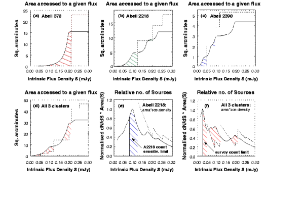
Figure 2: Increased sensitivity due to lensing: In (a), (b) and (c) the dashed line defines, per cluster field, the area of sky accessible to the survey as a function of flux in the absence of lensing. The profile is stepped because the rastering measurement performed on the sky covered different regions to different depth. The solid curve in each case shows how the area of sky covered depends on the limiting 15 $\mu$m flux after lensing is taken into account. (d) shows the same parameters for the composite survey which results from combining observations on the three clusters. In (e) and (f) the measured distribution of sources with flux density (dN/dS) has been folded with the previously illustrated flux-dependent accessible area in such a way that the resulting curves - (e) for the example of A2218 and (f) for the three-cluster survey - show the relative number of sources accessible to a lensing survey at each flux level. It is seen that a significant population of sources below the unlensed sensitivity limit (the dashed line) becomes accessible to the measurement. In each of (e) and (f) a solid vertical line delineates the 50% completeness limit for source counts. The dashed (unlensed) case also refers to the 50% completeness limit in the absence of lensing. The peaks in the source-density plots are due to the discontinuities in the sensitivity levels in the “accessible-areas” plots, arising from the raster measuring strategy used.

Fig. 2 illustrates an important benefit of observing through a gravitational lens. As described in the caption, it compares the surface areas of sky covered to a given limiting flux, with and without the action of the lensing cluster. The dashed lines in the figure refer to the unlensed case. The solid lines in Fig. 2.a through Fig. 2.d trace the relationship between achieved sensitivity and associated area surveyed, after correction for lensing gain. This is surface area in the source plane, or observed surface area corrected for lensing effects. It is seen that, as a result of lensing, it becomes possible to detect sources below the limits achievable in the absence of lensing. The flux-density domains in which these fainter sources become available are indicated by the hatched regions in the figure. However, to properly appreciate the benefit of the lensing survey it is necessary to consider, not simply the area of sky accessed to a given depth, but to fold in the number density of sources as a function of flux, in order to highlight the significant population of fainter sources made accessible by lensing. The result of this combination is represented by the shaded regions of Figs.2.e and 2.f, for the example of Abell 2218 and for the full three-cluster survey, respectively. To arrive at (e) and (f) the area accessed to a given flux has been folded with the 15 $\mu$m source density as a function of flux (i.e. with dN/dS). The subset of the overall source population made accessible by lensing is very significant in comparison with the subset of the population falling above the unlensed sensitivity threshold.

Lensing effects must be corrected during analysis (see Sec.4.8) in order to compare lensing results with unlensed sky counts (e.g. in the Hubble Deep Field and the Lockman Hole – Rowan-Robinson et al. 1997; Taniguchi et al. 1997; Aussel et al. 1999a; Elbaz et al. 1999 & 2002).

Table 1: Observational parameters and lensing clusters of galaxies used in the survey. On-chip integration time (t_int) was always 5.04 seconds and the 3 ^′′ per-pixel field-of-view was used. Sensitivity in $\mu$Jy is quoted at the 80% (and 50%) completeness limits, before taking account of the deepening achieved through the lensing amplification. In the table, M and N are the number of steps along each dimension of the raster. The increment for each raster step is denoted by dm and dn. Each raster was repeated k times.

Field	Filter †	Reads	n Steps	dm	dn	area	Max. depth ($\mu$Jy)	Done k	Tot. t
	$\lambda_{ref}$ $\mu$m	per step	M    N	′′	′′	${}^{\prime\prime^{-2}}$	80% (50%) complete	times	sec.
A2390	6.7	13	10    10	7	7	7	52 (38)	4	28488
	14.3	13	10    10	7	7	7	92 (50)	4	28493
A2218	6.7	14	12    12	16	16	20.5	79 (54)	2	22300
	14.3	14	12    12	16	16	20.5	167 (121)	2	22300
A370	6.7	10	14    14	22	22	40.5	80 (52)	2	22366
	14.3	10	14    14	22	22	40.5	293 (210)	2	22820

($\dagger$) 6.7 and 14.3 $\mu$m are, respectively, the reference wavelengths of the ISOCAM LW2 (7 $\mu$m) and LW3 (15 $\mu$m) filters, which have widths (5 to 8.5) $\mu$m and (12 to 18) $\mu$m.

3 Observations

3.1 Raster observations

The fields of the well-known gravitationally lensing galaxy clusters Abell 370, Abell 2218 and Abell 2390 were observed using the 7 $\mu$m (LW2: 5 to 8.5$\mu$m) and 15 $\mu$m (LW3: 12 to 18$\mu$m) filters of ISOCAM (Cesarsky et al. 1996). These filters employ the CAM long-wavelength (LW) detector, which was a 32 $\times$ 32 SiGa array. The fields were observed in raster mode. The parameters for the rasters and the details of the instrument configurations used are given in Table 1.

By employing the CAM 3^′′ per-pixel field-of-view (PFOV) and raster step sizes which were multiples of 1/3 of a pixel, over many raster steps, a final mosaic pixel size of 1″ was achieved. The diameter of the PSF central maximum at the first Airy minimum is 0.84$\times\lambda$($\mu$m)″.  The FWHM is about half that amount. More precisely, Okumura (1998) reports PSF FWHM values of 3.3″ at 7 $\mu$m and 5″ at 15 $\mu$m. The final 1″ pixel size improves resolution and allows better cross-identification with observations at other wavelengths. This strategy differs from many other CAM deep surveys which used the 6 ^′′ per-pixel field-of-view [for example the ELAIS survey (Oliver et al. 2000; Serjeant et al. 2000), the ISOCAM HDF (Rowan-Robinson et al. 1997), and the Lockman Hole survey (Taniguchi et al. 1997)].

The rasters achieve greatest depth around their centres because the dwell–time per position on the sky is a maximum in the centre of each raster. For purposes of data analysis and interpretation the rasters were divided into sensitivity zones. The total time required to execute each individual raster map is listed in Table 1. For the most sensitive, most redundant, rasters (on A2390) these are also the maximum per-pixel dwell-times for the inner regions of each raster, because the corresponding points on the sky “saw” the detector array for all raster positions. Execution times close to 30000 seconds represent rasters occupying a full half of an ISO revolution - this being the longest possible individual observation time with the spacecraft due to ground-station visibility constraints. Table 1 gives the limiting sensitivities achieved in each raster before correcting for the effects of cluster lensing.

Results obtained from a subset of the data employed in this paper have previously been reported by Altieri et al. (1999). Lémonon et al. (1998) reported results obtained from a shallower raster over A2390. Both groups used the reduction method called PRETI, described in Starck et al. (1999). Barvainis et al. (1999) reported CAM photometry of sources in the field of Abell 2218. The independent reduction method employed in the current work therefore enables a comparison of results obtained with different reduction strategies. As can be seen in Table 2, the results show excellent consistency within the 15 to 20% quoted precision.

Table 2: Comparison of 7 and 15 $\mu$m photometry from this paper with corresponding values from Lémonon et al. (1998) and Barvainis et al. (1999), for the few overlap cases. Column 1 lists the label assigned to each source in this paper. Columns 2 and 3 (L and B) give the identification numbers from the Lémonon and Barvainis papers respectively. Columns 4 and 7 list Lémonon et al. (1998) 15 and 7 $\mu$m photometry. Column 5 gives the Barvainis et al. (1999) photometry, and columns 6 and 8 give the photometry found in the tables later in this paper.

Source	L	B	Lémonon	Barvainis	Metcalfe	Lémonon	Metcalfe
			15 $\mu$m	15 $\mu$m	15 $\mu$m	7 $\mu$m	7 $\mu$m
			($\mu$Jy)	($\mu$Jy)	($\mu$Jy)	($\mu$Jy)	($\mu$Jy)
ISO_A2390_18	4		350${}^{+50}_{-40}$		382+/-59	110${}^{+40}_{-60}$	103+/-30
ISO_A2390_27	3		400${}^{+60}_{-50}$		321+/-58		153+/-21
ISO_A2390_28a	2		440${}^{+60}_{-60}$		461+/-58
ISO_A2390_37	1		500${}^{+80}_{-70}$		524+/-61	300${}^{+50}_{-40}$	361+/-26
ISO_A2218_27		395		1100+/-200	759+/-57		451+/-42
ISO_A2218_35		317		670+/-200	541+/-54		100+/-57
ISO_A2218_38		289		850+/-200	919+/-61		113+/-53
ISO_A2218_42		275		570+/-200	445+/-54		78+/-70

4 ISOCAM faint-source data reduction and analysis

4.1 General remarks

Methods and applications of ISOCAM data analysis directed at the extraction of the faintest sources have been described by Elbaz et al. (1998), Starck et al. (1999), Aussel et al. (1999a), and Lari et al. (2001).

Here we describe an independent method for extracting faint sources from ISOCAM data. The method can be readily applied by any user within the ISOCAM Interactive Analysis (CIA) system (Ott et al. 1997 & 2001; Delaney & Ott, 2002). Many of the steps developed have been incorporated into CIA as an indirect result of this work.

This section describes the steps required to achieve the removal of cosmic-ray induced glitches with first and second-order corrections, the correction of long-term signal drifts, compensation for short-term responsive transients, faint-source extraction and Monte-Carlo simulations to calibrate the faint-source data and assign completeness limits to the survey, and the method employed to correct the results for the effects of the lensing amplification of the cluster.

ISOCAM raw data takes the form of a cube comprised of large numbers of individual detector image frames, each frame corresponding to one readout of the full 32x32 detector array. A raw data cube may contain frames associated with more than one instrument configuration. The process of decomposing the data into configuration-specific structures is referred to as ”slicing” and is a standard reduction step provided for in the CAM Interactive Analysis system (Delaney & Ott, 2002; Ott et al. 1997). After slicing, one observation in one instrument configuration again takes the form of a cube of readouts. In the case of a raster measurement this cube can be decomposed into sub-units associated with each raster position. A source seen, perhaps repeatedly, by the detector as it rasters over the sky, will then appear in the data cube as pulsed signal buried in the data stream. The signal in an individual detector element, followed throughout the raster, may then typically take the form of a stream of signal recording the sky background, combined with dark-current, shot noise, irregular spikes induced by cosmic ray impacts (glitches), and possibly containing the quasi-periodic signature of sources seen during the raster. Even under stable illumination the signal from a given detector element may drift in time in a manner at least partly correlated with the illumination history of the array element. This occurs as the response of the detector element stabilises following any flux step associated with the start of the observation. Similar response drifts follow cosmic-ray induced glitches (see Fig. 3). Apart from the source-flux-induced drift behaviour, which can be modeled and corrected (Coulais & Abergel, 2000; Delaney & Ott, 2002), a lower level drift occurs at a few percent of the background signal. This long-term transient must be corrected by purely empirical means. The cumulative behaviour is manifested differently for each element of the detector array, since the elements differ in intrinsic sensitivity (i.e. the flat-field) and in their illumination and glitch histories.

It follows that the reduction of ISO faint source data is extremely challenging and many work-years have been invested in developing effective and reliable reduction techniques. The ultimate performance is particularly sensitive to the effectiveness with which the detector’s global responsive transient and the cosmic-ray-induced glitches can be removed from the data.

Figure 3: A typical time history for readout of a CAM LW detector pixel after primary deglitching. From the start of the sequence at image 0 the signal is seen to be subject to complex drifts. The spike around image 46 is the residue of a cosmic-ray-induced glitch left after initial deglitching. Another glitch residue near image 230 is followed by a severe dip in signal which recovers slowly (a “dipper” glitch). Between images 120 and 150 a faint source is detected. Its small, upward, signal growth-curve is characteristic of the short term responsive transient which affects sources at all flux levels in varying degrees. Truly faint sources, such as most of the sources discussed in this paper, are not immediately discernible in this way above the noise of such a single pixel data stream. This figure gives an indication of the challenges facing the efforts to accurately extract the faintest sources. Well established techniques exist to meet these challenges.

4.2 Initial reduction and first order deglitching

The data reduction begins as follows: after slicing, to render the data into instrument configuration-specific structures, the dark current is subtracted using a time-dependent dark model which takes account of a well characterised secular variation of current throughout the orbit (Biviano et al. 2000; Roman & Ott, 1999). The data-stream from each detector element is then deglitched using an iterative sigma clipping method which takes advantage of the fact that, for faint source work, the uniform celestial background flux dominates the measured signal while sources are very faint. Abrupt spikes and troughs in the data stream reveal the occurrence of glitches (rather than sources seen repeatedly (cyclically) during the raster).

Glitches are an important, and often dominant, limiting factor for all aspects of ISOCAM data analysis. However, primary glitch spikes often stand far above the already high background signal level. Sigma clipping around the average value of readouts of a pixel with such a perturbed history leads to a skewed clipping, because the mean value used as reference is severely perturbed.

For relatively stabilised (within a few percent of the asymptote) data, typical of the long-duration data sets used in this paper, the “Best Iterative Sigma Clipping Deglitcher” (BISC) was developed. It applies an iterative method consisting of four basic steps:

1. for each raster-position, the flux per pixel is estimated

2. the data vector, which covers many raster positions, is normalised by subtracting this flux estimate, reducing the effect of signal drifts in comparison with glitches

3. the variance of the normalised data vector is computed

4. outliers are identified by sigma clipping

5. a new (and now improved) estimate of the flux per pixel is made, masking the outliers, and the process is repeated until the flux level of each pixel in each raster-position reaches a stable value.

Clipping of the original data vector based upon its mean and standard deviation, with the glitched elements masked, results in a good rejection of glitch spikes with minimum loss of valid data points.

Very long glitches, referred to as faders and dippers (see Fig. 3), can induce long-lasting signal gradients seen strongly in the background signal. To identify and reject these, the mean and variance of the slope per pixel and raster-position are computed. Data showing a consistent upward or downward trend are rejected as being of low quality.

4.3 Removal of short and long–term transients

After this first-order deglitching the data cube is flat-fielded using the median frame from the entire raster, but excluding the initial strong responsive transient which follows the establishment of the observing configuration. At this stage an inspection of the data stream from an individual detector element will typically show a smoothly varying signal with residual glitch spikes and troughs (see Fig. 3). These two remaining characteristics, temporal variation and residual glitches, represent the fundamental challenge to the successful extraction of faint point sources.

The temporal drift is decomposed as follows : (a) a “short-term” responsive transient following changes in incident illumination on a detector element (e.g. the onset of a source - see Fig. 3), (b) short term responsive perturbations following cosmic-ray induced glitches, & (c) a long-term responsive transient in the measured background, at a level of a few percent of the background.

The three sources of drift are corrected as follows :

(a) ”Short-term” responsive transients

The responsive transient which occurs, for example, whenever a source moves onto a new pixel causes the source signal as recorded by that pixel to appear roughly like a growing exponential curve (in appearance, somewhat like the charging-curve of a capacitor, though not having the same functional form). This response will, in general, not have stabilised before the raster carries the source on to some other detector pixel. The result is that the cumulative signal from that source over the full raster will be suppressed relative to the value it would have if the signal were allowed to stabilise on each detector pixel. This effect can be corrected by applying a physical model to the data–stream for each detector pixel. However, such application causes a reduction in the S/N in the final raster mosaic. For this reason we reduce the rasters without applying the model correction for the short-term transient, and so recover the maximum number of faint sources. We then separately reduce the data applying the transient model and compare the results achieved in this way with those obtained without transient modeling, so deriving a global correction factor to apply to all sources in the non-transient-corrected map.

(b) The correction for short term responsive perturbations following cosmic-ray induced glitches, and other glitch residues is discussed in Sec.4.4, below.

(c) ”Long-term” responsive transients

The low-level long-term signal drift is not significant in terms of photometric accuracy. However, it leads to an apparent illumination gradient of one or two percent of the background across the reconstructed raster maps, and this is sufficient to swamp faint point sources given the high background characteristic of most ISO bandpasses. We have found entirely satisfactory results removing the long-term drift by simply fitting the signal-stream from each detector pixel with a broad running median, and then subtracting the smoothed signal history from the unsmoothed version. The signal-stream from each detector pixel consists of many readouts of the pixel, with typically 10 to 15 readouts corresponding to one raster position (Table 1). The filtering suppresses the long-term drifts and any large scale extended structure. However, provided the width of the running-filter is several times the number of readouts associated with a raster position the record of point sources in the data-stream is preserved. We describe below extensive Monte-Carlo simulations which allow us to compensate for any residual perturbations of photometry which might arise due to this filtering procedure, and due to the overall processing chain in general.

After subtraction of the smoothed time history from the unsmoothed data the signal history of each detector pixel takes the form of noise scattered about zero, interspersed with weak point-source detections and glitch residues.

4.4 Removal of glitch residues - Second-order deglitching

First-order deglitching, described above, removes glitch spikes from the data-stream generated in individual detector pixels. That deglitching process is not perfect. It may leave residues of glitches in the data-stream which can resurface in the final raster mosaic and mimic faint point-sources. The first-order deglitching takes no account of the fact that a given celestial source will, in general, be seen by many detector pixels in the course of a full raster observation. The number of times a source is seen by different detector pixels is referred to as the raster redundancy for that source. The fact that actual sources are multiply detected while glitches are isolated events allows discrimination of real faint sources from glitch residues.

The data cube is reorganised as follows to facilitate this discrimination. For each raster position the corresponding detector readouts are averaged to yield a single image. A large data cube is created having the X and Y dimensions corresponding to the full raster mosaic on the sky. In the end, each (x,y) coordinate of this cube represents one pixel on the sky. The Z dimension is the number of raster positions in the raster map. The raster-position-images are then placed into this ”sky-cube” in such a way that the first plane of the sky-cube holds the image from the first raster position, the second plane of the sky-cube holds the image from the second raster position displaced laterally in the cube by an amount equal to one raster step, the third plane of the sky-cube holds the image from the third raster position, and this process is continued until the full sky-cube is produced. The corresponding Z track through the cube, for pixel (x,y), traces each of the occasions on which that sky-pixel was seen by some detector pixel. If the raster caused the detector to move completely off some patch of sky then the corresponding part of the sky cube will contain zeros or undefined values which will be ignored in further data reduction.

If one chooses some (x,y) in the sky map, the corresponding vector defined by looking down the Z-axis of the cube is a time history of samples for that sky-pixel. The Z vector will consistently record enhanced signal when that sky pixel corresponds to a source. Glitch residues appear as spikes on top of this constant source signal and can be efficiently rejected by sigma-clipping. Sigma clipping with a two-sigma threshold is possible without having any significant effect on the source photometry because all samples for such a sky-pixel represent flux measurements on the same source. The extensive Monte-Carlo simulations validate and calibrate this process.

Once all of the above reduction steps have been completed the raster data cube can be collapsed to produce the final raster map of the target field.

4.5 Point-source extraction

Sources listed in this paper fall into two categories: (i) sources included in the photometric lists, and (ii) sources more stringently screened for inclusion in the statistical source counts.

Case (i): for inclusion only in photometric lists detections are accepted as real which either (a) are confirmed by eye on at least two separate IR maps (almost always the case for sources listed in this paper) or which (b) in the case of a very few sources near the noisy edges of the map, may fall off the edge of one map due to small deliberate mutual displacements of successive rasters on the same field, but which have clear optical counterparts. All sources listed in this paper have optical counterparts. In a few cases these are quite faint - at the limits of the deepest ground-based observations.

Case (ii): it was necessary that point-sources to be used for source counting be extracted by automatic and objective means in order to impart well defined statistical properties to the sample.

The following method was adopted to extract the list of sources for the source counts, and to characterise the statistical properties of that sample:

• First, the real sources in a given field were identified independently of the automatic extraction process by identifying as real those sources which were visually confirmed on at least two independent raster maps, and which have optical counterparts. Not all sources identified in this way are counted!

• The parameters of the automatic source extraction tool, SExtractor (Bertin & Arnouts, 1996) were then tuned for each map to reproduce as closely as possible the above set of real sources. Only the set of sources detected in this manner are available for source counting. Sources not found using the chosen settings of SExtractor (only a few percent of the real sources) are listed among the uncountable sources at the end of each photometric table later in this paper. The small attrition is not a problem, indeed it must be accepted in order to benefit from the intrinsic objectivity of the automatic process. It simply means that the source extractor is tuned to detect some signal levels of the underlying source population with less than 100% completeness.

• Fake source Monte-Carlo simulations (described in detail in the following section) are then performed to calibrate the completeness characteristics of the automatically and rigourously selected source sample as a function of source brightness, and in the process to characterise the signal transfer function of the data reduction algorithm.

4.6 Monte-Carlo “fake-source” simulations

In what follows we will use the terms “real” data to designate data recorded during the actual in-flight measurements. “Fake” sources are model point sources inserted into the real data for purposes of simulation. A detection derived from an actual source on the sky is termed a real source, as defined in the previous section. An apparent detection derived from a cosmic-ray glitch or noise spike is termed a “false” detection. False detections are rejected with high efficiencey because (a) they do not meet the criteria specified above for identification as real sources, and (b) they do not correspond to any known, inserted, fake source.

The Monte-Carlo simulations address two questions:

• What fraction of a well defined source population is recovered by the source extractor to given signal limits. i.e. what is the completeness of the survey to different signal limits.

• how does signal in the final map relate to signal in the raw data.

Extensive fake-source simulations were performed as follows to address the above issues:

Artificial point sources, which were filter-specific models of the CAM PSF (Okumura 1998), were inserted into the individual detector readouts of the raw data cubes for the observations. These fake sources were inserted into regions of the cube free of real sources. The positions of the fake sources within the source-free regions of the data frames for a given simulation were determined by a random number generator. For any given raster observation a total of typically one thousand fake sources were inserted into the raw data through 100 independent simulations.

For each individual simulation, ten fake sources were inserted into the raw raster cube, all with the same signal level. Then the data were reduced through the full reduction process, including automatic source extraction. Fake sources and real sources face exactly the same reduction steps.

The simulation was then repeated for ten new fake sources at new positions. This process was repeated for typically ten ensembles of sources and further repeated for typically ten to twenty different signal levels of the sources.

For each fake-source signal level in the raw data the fraction of signal recovered during source extraction on the final map was determined. This allows recovered signal to be correlated with signal in the raw data cube over the full range of signal levels spanned by the real sources.

For each fake-source signal level in the raw data the fraction of the total number of inserted fake-sources that were recovered during the source extraction process was determined, so establishing the completeness of the map to that signal level.

4.7 Correlation of detector signal with actual flux density

Now in each of the above cases the properties of sources in the final map are correlated, through the simulation, with source signal in the raw data, rather than with source brightness on the sky. To establish the correlation with source flux on the sky, as opposed to signal in the detector, the transformation from source signal in the raw data, measured in ADU (Analogue-to-Digital Units), to mJy on the sky, is needed.

We treat this transformation as having two components as follows. First, the ISOCAM instrument teams determined through the mission the filter-specific transformation from ADU to mJy for a source which has been seen by the detector long enough for its signal to have stabilised. The CAM Interactive Analysis (CIA) system (Delaney & Ott, 2002) contains these factors, and the ISO Handbook Volume III (CAM) (Blommaert et al. 2001) describes and lists them for all CAM filters, as derived from hundreds of calibration measurements throughout the ISO operational mission.

Second, since our detections refer to sources which have been seen by any given detector pixel for on-the-order-of only ten readouts, their signals have not stabilised completely. The inserted fake-sources do not attempt to model this transient response behaviour, therefore a scaling factor must be applied, on top of the standard calibration factor just described, in order to correctly relate source signal in the raw data to mJy. The method for determining this additional scaling factor has been described in Sec.4.3 above (Coulais & Abergel, 2000).

In the end, if n ADU per unit electronic gain per second of point-source signal is detected within the photometric aperture on the final map, this is related to source strength in mJy by the transformation : $S=n\times f\times R\times T$

• n = source signal in detector units (ADU/gain/second) derived by aperture photometry in the final map (a 9 arcsecond aperture was used in all cases)

• f = the photometric scaling function, determined by simulations. It relates measured signal in a photometric aperture to total point source signal

• R = the standard photometric scaling factor relating signal in the detector for stabilised data to flux on the sky and taken from the ISOCAM Handbook as described above [units mJy/(ADU/g/s)]

• T = responsive transient scaling factor: i.e. the ratio [stabilised_signal/unstab_signal] for the particular measurement in question, derived by reference to a physical model (see Sec.4.3 (Coulais & Abergel, 2000)).

4.8 Correction for the gravitational lensing amplification

As has been discussed earlier in this paper, the advantage of using clusters of galaxies as natural telescopes is that it becomes possible to probe fainter and more distant sources than would otherwise be reachable in the same time with standard techniques. However, source fluxes, and the effective area of sky surveyed, have to be corrected for the effects of the lensing amplification. The necessary corrections require a good knowledge of the mass distribution of the clusters based on multiple images of background sources with measured redshift. These allow accurate probing of the mass distribution of the lensing cluster. Detailed lensing models of the three clusters used here have been computed (Kneib et al. 1996, Pelló et al. 1999, and Bézecourt et al. 1999). The correction technique is now well tested and has been applied on different catalogues of faint sources, e.g. by Blain et al. (1999) and by Cowie, Barger & Kneib (2002) on the submillimetre faint lensed galaxy population, and by Smith et al. (2002) on the lensed ERO galaxy population.

We face a further complication in determining the area surveyed to a given flux. In addition to the fact that the lensing-amplification-corrected detection sensitivity depends on position within the map, the apparent detection sensitivity is also non–uniform and depends upon position in the final image. This is a consequence of the rastering observing strategy needed to cover sufficient area while obtaining a good flat-field. This effect is not critical for wider field observations, like the Abell 370 case, but becomes important for the Abell 2390 observation, where the number of measurement samples per sky position varies strongly from the centre to the edge of the map. However, this variation in measurement sensitivity is highly regular over the map due to the uniform geometrical character of the raster, and the Monte Carlo simulations, which probe sensitivity from region to region within the maps, suffice to fully take it into account.

In addition to the above, the redshift distribution of the observed mid-Infrared sources is broad, with available measured redshifts ranging up to z=2.8 and with the redshift distribution of the lensed sources peaking around z $\simeq 0.7$. The value of the lensing amplification depends on redshift. For those sources for which a measured redshift was not available, we have employed the method described in Sec.6.1.1 to sort the sources into cluster and non-cluster objects, and for the sources deemed to be background sources the median redshift of the sample, $z\,\sim\,0.7$, has been assigned.

To compute the source counts corrected for the effects of lensing, the lensing amplification is computed for each source using the cluster mass model in order to determine the unlensed flux density of the source. Then we compute in the corresponding source plane the area surveyed at the completeness limit (flux limit) applicable to the source measurement, taking into account the fact that the detection sensitivity on the sky (in the image plane) is not uniform due to the rastering measurement. I.e. different sensitivities apply to different regions of the maps, so some regions are not viable at some flux levels. The inverse of the area surveyed for a given source (a given flux level), multiplied by the completeness correction for that flux level, gives the source count for that lensing corrected source flux. Binning and summing these results allows us to derive the differential and cumulative source counts corrected for the effects of lensing. The cumulative unlensed source counts are presented and discussed in Sec.6.

5 Results - Images and Photometry

In this section we present maps of the fields observed showing IR contours at 7 and 15 $\mu$m overlaid on optical images, and also tables of the 7 and 15 $\mu$m sources detected for each of the three cluster fields, giving measured coordinates and flux densities. The coordinates are those measured by ISOCAM, and may have an apparent, cluster/filter dependent, systematic offset of a few arcseconds from the optically determined coordinates of their counterparts.

5.1 Cluster images at 7 and 15 $\mu$m

The areas of sky covered in the cluster fields are listed in Table 1. The mid-infrared sources are labeled in each map in order of increasing RA. The noise level increases towards the edges of the ISOCAM maps.

Figures 4, 6 and 8 show the 7 $\mu$m deep images of the three lensing cluster fields. Figures 5,  7 and  9 show the 15 $\mu$m maps. Spatial resolution of the ISO maps is sufficiently good to allow identification of IR correlations with the optical morphology of objects. For example the ISO source ISO_A2390_28a in Fig. 9 matches the bright optical knot in the straight arc (Pelló et al. 1991) near the centre of the A2390 map. From these images we can remark that the optical arc(lets) are generally not detected at mid-infrared wavelengths. Yet large numbers of mid-infrared sources that spectroscopic, photometric or lensing redshifts show to be behind the lens are detected. Thanks to our comparatively high-resolution images the correlation of ISO sources with (sometimes extremely faint) optical counterparts in deep NIR and optical images (e.g. from HST/WFPC2 or ground-based telescopes) has been quite straightforward. We found that at 7 $\mu$m the bulk of the sources are cluster galaxies, the rest are lensed background sources, field sources, or stars. Most 15 $\mu$m sources for which spectroscopic redshifts are available are found to be lensed background galaxies. The photometric and lensing-inversion redshifts for the remaining sources, where available, are consistent with this conclusion. At 15 $\mu$m, the cluster-core essentially disappears.

Figure 4: Contours of the ISOCAM 7 $\mu$m image of Abell 370 (z = 0.37) overlaid on a deep CFHT I-band image (also used in figure 5). Sources are labelled in order of increasing RA. The + sign identifies sources detected at 7 $\mu$m but not at 15 $\mu$m. If the ID number of a source is enclosed within a square then the source has been detected at X-ray wavelengths in Chandra data (Bautz et al.  2000). If the ID number of a source is enclosed within a circle then the source has been detected at submm wavelengths with SCUBA (Ivison et al. 1998; Smail et al. 2002; Cowie et al. 2002). The giant arc (near foreground source 11b) is barely detected at 7 $\mu$m, but the two giant ellipticals (11c and 12) at the centre of A370 are both detected. Source 18 falls off this map and its approximate location is simply indicated by an arrow. Axes are labelled in arcseconds. North is to the top and East to the left. The ISO raster was centred at approximately R.A. 02 39 52.9 DEC -01 35 05 (J2000).

Figure 5: Contours of an ISOCAM 15 $\mu$m image of Abell 370 (z = 0.37) overlaid on a deep CFHT I-band image. The sources are labeled in order of increasing RA. The - sign identifies sources detected at 15 $\mu$m but not at 7 $\mu$m. If the ID number of a source is enclosed within a square then the source has been detected at X-ray wavelengths in Chandra data (Bautz et al.  2000). If the ID number of a source is enclosed within a circle then the source has been detected at submm wavelengths with SCUBA (Ivison et al. 1998; Smail et al. 2002; Cowie et al. 2002). The giant arc (source number 11) is well detected by ISO. Some of the mid-IR sources have quite faint optical counterparts. Axes are labelled in arcseconds. North is to the top and East to the left. The ISO raster was centred at approximately R.A. 02 39 52.9 DEC -01 35 05 (J2000).

Figure 6: Contours of an ISOCAM 7 $\mu$m image of Abell 2218 (z = 0.18) overlaid on a deep Palomar 5m I-band image (Smail, private communication). The sources are labeled in order of increasing RA. The + sign identifies sources detected at 7 $\mu$m but not at 15 $\mu$m. If the ID number of a source is enclosed within a square then the source has been detected at X-ray wavelengths in Chandra archival images. Axes are labelled in arcseconds. North is to the top and East to the left. The ISO raster was centred at approximately R.A. 16 35 55.7 DEC 66 12 30 (J2000).

Figure 7: Contours of an ISOCAM 15 $\mu$m image of Abell 2218 (z = 0.18) overlaid on a deep Palomar 5m I-band image (Smail, private communication). The sources are labeled in order of increasing RA. The - sign identifies sources detected at 15 $\mu$m but not at 7 $\mu$m. If the ID number of a source is enclosed within a square then the source has been detected at X-ray wavelengths in Chandra archival images. Note the strong ISO detection of the giant arc (number 38), the several mid-infrared sources corresponding to faint optical counterparts [e.g. 43, 67] and the fact that the IR “arclets” are generally not from the same population as the known optical arclets. Source 27 is a foreground galaxy. Axes are labelled in arcseconds. North is to the top and East to the left. The ISO raster was centred at approximately R.A. 16 35 55.7 DEC 66 12 30 (J2000).

Figure 8: Contours of an ISOCAM 7 $\mu$m image of Abell 2390 (z = 0.23) overlaid on a KPNO R-band image (Soucail, private communication). The sources are labeled in order of increasing RA. The + sign identifies sources detected at 7 $\mu$m but not at 15 $\mu$m. If the ID number of a source is enclosed within a square then the source has been detected at X-ray wavelengths in Chandra data (Fabian et al. 2000; Wilman et al. 2000a). If the ID number of a source is enclosed within a circle then the source has been detected at submm wavelengths with SCUBA (Smail et al. 2002; Cowie et al. 2002). Axes are labelled in arcseconds. North is to the top and East to the left. The ISO raster was centred at approximately R.A. 21 53 33.9 DEC 17 42 00 (J2000).

Figure 9: Contours of an ISOCAM 15 $\mu$m image of Abell 2390 (z = 0.23) overlaid on a KPNO R-band image (Soucail, private communication). The sources are labeled in order of increasing RA. The - sign identifies sources detected at 15 $\mu$m but not at 7 $\mu$m. If the ID number of a source is enclosed within a square then the source has been detected at X-ray wavelengths in Chandra data (Fabian et al. 2000; Wilman et al. 2000a). If the ID number of a source is enclosed within a circle then the source has been detected at submm wavelengths with SCUBA (Smail et al. 2002; Cowie et al. 2002). Note the ISO detection of part of the straight arc near the centre of the image (source number 28a), and the two strong ISO detections of the optically very faint sources 18 and 25. These objects have extremely red colours and very faint visual fluxes. Axes are labelled in arcseconds. North is to the top and East to the left. The ISO raster was centred at approximately R.A. 21 53 33.9 DEC 17 42 00 (J2000).

Some ISO targets have extremely red optical and NIR colours. It appears that 15 $\mu$m imaging favours selection of star-forming galaxies and dusty AGNs that are not evident in UV/optical surveys.

5.2 Photometry

Table 3 lists, for all clusters and both bandpasses, the sensitivities achieved to three completeness levels (90%, 80% and 50%) in each of the sensitivity zones defined for each raster. The areas of the zones are given in square arcseconds. The zones are labeled a, b, c, and d, and represent steps of a factor of 2 in observation dwell–time per sky pixel (or raster redundancy per pixel). The low redundancy noisy “a”-regions were excluded from contributing to the source counts, but contributed sources to the photometric lists.

Table 3: Sensitivities achieved in the survey. For each cluster in each filter the raster is divided into zones a to d. Zone d is the inner, most redundant and sensitive region. Zone a is the outer, least redundant and sensitive region. The limiting flux for detections with 90%, 80% and 50% completeness, and the area covered, is given in square arcseconds for each zone.

Field	Filter †	Zone	Depth (mJy)			Zone	Tot. Usable
			90%	80%	50%	Area	Area
						[$\prime\prime^{2}$]	[$\prime\prime^{2}$]
	LW2	a	0.163	0.149	0.107	6135
		b	0.087	0.08	0.06	5154
		c	0.063	0.059	0.046	6835
		d	0.057	0.052	0.038	7157	25281
Abell 2390	LW3	a	0.475	0.392	0.220	6125
		b	0.415	0.281	0.116	5192
		c	0.140	0.128	0.092	6804
		d	0.107	0.092	0.050	7160	25281
	LW2	a	0.294	0.268	0.180	9728
		b	0.180	0.166	0.124	13564
		c	0.112	0.103	0.078	19004
		d	0.087	0.79	0.054	31688	73984
Abell 2218	LW3	a	0.449	0.412	0.300	9608
		b	0.328	0.309	0.251	13319
		c	0.266	0.249	0.198	19100
		d	0.186	0.167	0.121	31957	73984
	LW2	a	Insufficient redundancy			10187
		b	Insufficient redundancy			21344
		c	0.135	0.124	0.09	32579
		d	0.1	0.08	0.052	81814	114393
Abell 370	LW3	a	Insufficient redundancy			9434
		b	Insufficient redundancy			22358
		c	Insufficient redundancy			31808
		d	0.331	0.293	0.21	82324	82324

($\dagger$) LW2 and LW3 filters have reference wavelengths 6.7 and 15 $\mu$m, respectively.

The photometry for the 145 mid-infrared background, cluster and foreground sources detected in the survey is listed in Tables 4 to 9. For each table, the significance of the columns is as follows :

Column 1 gives the source identifier. A minus sign beside the source number indicates a source seen only at 15 $\mu$m. A plus sign indicates a source seen only at 7 $\mu$m. Column 2 gives the source signal in detector units with the precision in detector units listed in Column 3. The square brackets in Column 4 enclose the value of the significance of the detection with reference to the local background noise in the map. The significance is not the same as the signal divided by the precision. The precision includes factors roughly dependent on source signal (for example due to cosmic-ray induced glitches which change the detector responsivity) and which affect the accuracy of the flux determination. The significance is the ratio of the source signal to the 1-sigma local noise floor of the map as derived from the Monte-Carlo simulations (the scatter on the recovered signal of the faintest fake sources recovered with greater than 50% completeness). The distinction is clearly understood if one considers a bright source affected by a glitch (limited precision but high significance). Column 5 gives the flux density of the source in mJy, with the associated precision listed in Column 6. Column 7 gives the intrinsic flux density of the source after correction for lensing amplification, with the associated precision listed in Column 8, which is the quadrature sum of the apparent flux precision with an estimate of the accuracy of the lensing amplification model at the source location. (The absoulte uncertainty on the intrinsic flux-density is smaller than the absoulte uncertainty on the apparent flux-density because of the lensing factor, but the fractional error on the intrinsic flux-density is, of course, increased by the quadrature summation of errors.) Columns 9 and 10 list the Right Ascenscion and Declination in J2000 coordinates, as determined by the ISO Attitude and Orbit Control System (AOCS). Due to jitter in the positioning of ISOCAM’s lens wheel the inherent accuracy of the AOCS ($\sim$3″ ) was not always achieved, and these coordinates may differ systematically by a few arcseconds (typically less than 6″) from the coordinates of optical counterparts, with map dependent offsets being needed from map to map to align the ISO images with the optical data. Column 11 lists the spectroscopic redshift for the source, if known, along with a key indicating the origin of the z information. The key is decoded at the end of each table. Where no redshift information is available sources are sorted into cluster-member and non-cluster-member background-source categories based on their IR colours, as mentioned above in Sec.4.8 and described in detail in Sec.6.1.1. As already stated in Sec.4.8, sources identified as background sources in this way are assigned a redshift of 0.7, roughly the median value for the 15 $\mu$m background population.

Each 15 $\mu$m table is organised into three sections vertically, separated by blank rows across the table. The upper section lists the sources meeting all of the criteria for countability, and detected above the 80% completeness threshold. The middle section lists the sources meeting all of the criteria for countability, and detected above the 50% completeness threshold. The bottom section of each table lists the sources rejected for counting (as cluster members or as stars) or detected below the 50% completeness threshold. In all cases the significance of the detection is given.

The 7 $\mu$m tables are divided into two sections vertically, separated by a blank row across the table. The upper section lists the sources meeting all of the criteria for countability, and detected above the 80% completeness threshold. The bottom section of each table lists the sources rejected for counting (as cluster members or as stars) or detected below the 80% completeness threshold. In every case the significance of the detection is given.

Table 4: 15 $\mu$m sources detected in the field of Abell 370. The significance of the columns is explained in the text (Sec.5.2). Horizontal blank lines divide the table into three parts. The upper section holds non-cluster sources detected above the 80% completeness limit. The middle section holds non-cluster sources detected above the 50% completeness limit. The bottom section holds cluster sources and any non-cluster sources not meeting statistical criteria for inclusion in the counts. (See Sec.4.5 & Sec.4.6.) When the redshift is given in italics it has been assigned to 0 for stars, or to the median redshift of the background population, $\sim$0.7, for background objects lacking spectroscopic redshift (see Sections 6.1.1 and 7.1), or the source is in the cluster. The letters associated with z values identify the origin of the z value, expanded at the end of the table. Source IDs accompanied by (-) signs are sources detected at 15 $\mu$m, but not at 7 $\mu$m. The mean redshift of the cluster is z = 0.374.

Object ID	S	Precision		F	Precision	Lens corr.	Precision	R.A.	DEC	zspec
ISO_A370	(ADU)	(ADU) &		(mJy)	+/-mJy	F (mJy)	+/-mJy			if known
		Significance			(1$\sigma$)		(1$\sigma$)
		[$S/\sigma_{floor}$]
01 -	0.325	0.062	[8.5 ]	0.361	0.280	0.325	0.070	2: 39: 45.6	-1: 33: 13	0.700
03 -	0.560	0.064	[14.7]	0.656	0.080	0.615	0.077	2: 39: 48.1	-1: 33: 26	0.44K
08 -	0.395	0.059	[10.3]	0.449	0.074	0.449	0.074	2: 39: 51.7	-1: 35: 16	0.306M
09	0.399	0.059	[10.5]	0.454	0.074	0.198	0.040	2: 39: 51.7	-1: 35: 52	2.803I
10 -	0.314	0.057	[8.3 ]	0.347	0.071	0.331	0.070	2: 39: 51.7	-1: 36: 09	0.42K
11 -	1.08	0.285	[28.4]	1.300	0.360	0.200	0.060	2: 39: 53.0	-1: 34: 59	0.724S8
15	0.434	0.058	[11.4]	0.498	0.073	0.498	0.073	2: 39: 54.4	-1: 32: 28	0.045N
16 -	0.346	0.061	[9.1 ]	0.388	0.077	0.357	0.071	2: 39: 55.9	-1: 37: 01	0.700
17	1.148	0.062	[30.2]	1.395	0.078	0.788	0.080	2: 39: 56.4	-1: 34: 21	1.062S9/B
19 -	0.279	0.057	[7.3 ]	0.303	0.071	0.278	0.066	2: 39: 56.9	-1: 36: 49	0.700
21 -	0.705	0.285	[18.6]	0.840	0.360	0.780	0.080	2: 39: 58.0	-1: 32: 26	0.700
23 -	0.318	0.061	[8.4 ]	0.352	0.077	0.320	0.071	2: 40: 00.1	-1: 35: 34	0.700
02 -	0.239	0.047	[6.3 ]	0.253	0.059	0.238	0.056	2: 39: 46.3	-1: 36: 48	0.700
20 -	0.218	0.047	[5.7 ]	0.227	0.059	0.196	0.051	2: 39: 57.5	-1: 33: 16	0.700
24 -	0.26	0.047	[6.8 ]	0.280	0.059	0.258	0.055	2: 40: 00.6	-1: 33: 44	0.700
25 -	0.262	0.047	[6.9 ]	0.282	0.059	0.282	0.059	2: 40: 00.8	-1: 36: 11	0.23M
04 -	0.203	0.038	[5.3 ]	0.208	0.047	0.152	0.035	2: 39: 48.6	-1: 35: 14	0.700
05 -	0.203	0.038	[5.3 ]	0.208	0.047	0.154	0.036	2: 39: 49.4	-1: 35: 33	0.700
14 -	0.384	0.059	[10.1]	0.435	0.074	0.435	0.074	2: 39: 54.3	-1: 33: 30	0.375M
22	0.55	0.064	[14.5]	0.644	0.080	0.644	0.081	2: 39: 59.0	-1: 33: 55	0 star
Redshift references : S8 = Soucail et al. 1988; M = Mellier et al. 1988; I = Ivison et al. 1998.
S9 = Soucail et al. 1999; B = Barger et al. 1999; K = Kneib, unpublished; N = NED

Table 5: 15 $\mu$m sources detected in the field of Abell 2218. The significance of the columns is explained in the text (Sec.5.2). Horizontal blank lines divide the table into three parts. The upper section holds non-cluster sources detected above the 80% completeness limit. The middle section holds non-cluster sources detected above the 50% completeness limit. The bottom section holds cluster sources and any non-cluster sources not meeting statistical criteria for inclusion in the counts. (See Sec.4.5 & Sec.4.6.) When the redshift is given in italics it has been assigned to 0 for stars, or to the median redshift of the background population, $\sim$0.7, for background objects lacking spectroscopic redshift (see Sections 6.1.1 and 7.1), or the source is in the cluster. The letters associated with z values identify the origin of the z value, expanded at the end of the table. Source IDs accompanied by (-) signs are sources detected at 15 $\mu$m, but not at 7 $\mu$m. The mean redshift of the cluster is z = 0.1756.

Object ID	S	Precision		F	Precision	Lens corr.	Precision	R.A.	DEC	zspec
ISO_A2218	(ADU)	(ADU) &		(mJy)	+/-mJy	F (mJy)	+/-mJy			if known
		Significance			(1$\sigma$)		(1$\sigma$)
		[$S/\sigma_{floor}$]
02	0.363	0.016	[21.2]	0.472	0.028	0.406	0.030	16: 35: 32.2	66: 12: 02	0.53K
08 -	0.306	0.019	[18]	0.393	0.026	0.249	0.034	16: 35: 37.2	66: 13: 12	0.68K
13 -	0.314	0.019	[18.5]	0.404	0.026	0.222	0.037	16: 35: 40.9	66: 13: 30	0.700
15a -	0.279	0.041	[16.4]	0.368	0.054	0.222	0.044	16: 35: 42.1	66: 12: 10	0.700
17	0.134	0.046	[7.9]	0.177	0.061	0.115	0.042	16: 35: 43.7	66: 11: 54	0.700
19 -	0.213	0.017	[12.5]	0.264	0.024	0.208	0.024	16: 35: 44.4	66: 14: 23	0.72K
27	0.575	0.046	[34]	0.759	0.057	0.759	0.057	16: 35: 48.8	66: 13: 00	0.103L2
35	0.41	0.041	[24]	0.541	0.054	0.204	0.050	16: 35: 53.2	66: 12: 57	0.474Eb
38	0.696	0.046	[41]	0.919	0.061	0.222	0.064	16: 35: 54.9	66: 11: 50	1.034P
42	0.337	0.041	[20]	0.445	0.054	0.274	0.048	16: 35: 55.3	66: 13: 13	0.45K
43 -	0.349	0.019	[20.5]	0.452	0.028	0.367	0.031	16: 35: 55.4	66: 10: 30	0.700
46 -	0.137	0.046	[8.1]	0.181	0.061	0.144	0.049	16: 35: 56.6	66: 14: 03	0.700
48	0.214	0.045	[12.6]	0.283	0.059	0.248	0.053	16: 35: 57.2	66: 14: 37	0.700
50 -	0.353	0.051	[10.7]	0.415	0.073	0.364	0.066	16: 35: 57.5	66: 10: 08	0.700
51	0.188	0.045	[11]	0.248	0.059	0.132	0.038	16: 35: 58.0	66: 11: 11	0.700
52	0.358	0.041	[22]	0.473	0.054	0.178	0.044	16: 35: 58.7	66: 11: 47	0.55K
53 -	0.341	0.041	[20]	0.450	0.054	0.113	0.034	16: 35: 58.8	66: 11: 59	0.693Eb
61a	0.14	0.046	[8.2]	0.185	0.061	0.136	0.061	16: 36: 03.6	66: 13: 32	0.700
65 -	0.657	0.031	[38.1]	0.878	0.043	0.734	0.052	16: 36: 05.1	66: 10: 43	0.64K
67	0.27	0.041	[15.9]	0.356	0.054	0.259	0.045	16: 36: 06.4	66: 12: 30	0.700
68	0.221	0.044	[13]	0.292	0.058	0.247	0.050	16: 36: 07.2	66: 12: 59	0.42K
69 -	0.137	0.046	[8]	0.181	0.061	0.135	0.047	16: 36: 07.6	66: 12: 21	0.700
73b -	0.284	0.046	[8.6]	0.326	0.060	0.292	0.055	16: 36: 10.3	66: 13: 48	0.700
09 -	0.168	0.017	[10]	0.202	0.024	0.111	0.021	16: 35: 39.0	66: 13: 07	0.68K
10 -	0.098	0.037	[5.8]	0.129	0.049	0.091	0.036	16: 35: 39.4	66: 12: 05	0.700
26 -	0.093	0.037	[5.5]	0.123	0.049	0.056	0.025	16: 35: 48.2	66: 12: 01	0.700
29 -	0.112	0.044	[6.6]	0.148	0.049	0.079	0.029	16: 35: 49.6	66: 13: 34	0.521Eb
37 -	0.117	0.037	[6.9]	0.154	0.049	0.109	0.036	16: 35: 54.8	66: 10: 53	0.700
44 -	0.101	0.037	[6]	0.133	0.049	0.086	0.033	16: 35: 55.7	66: 13: 28	0.596Eb
05 -	0.208	0.046	[6.3]	0.227	0.060	0.164	0.046	16: 35: 34.3	66: 13: 11	0.700
06	0.128	0.017	[7.5]	0.147	0.024	0.147	0.024	16: 35: 34.7	66: 12: 32	0.180L2
07 -	0.203	0.046	[6.1]	0.220	0.060	0.151	0.043	16: 35: 36.4	66: 13: 31	0.700
20 -	0.068	0.037	[4]	0.090	0.049	0.018	0.011	16: 35: 44.7	66: 12: 45	0.475Eb
25 -	0.103	0.037	[6]	0.136	0.049	0.136	0.049	16: 35: 48.3	66: 11: 26	0.1741L2
30	0.13	0.046	[7.6]	0.172	0.058	0.172	0.058	16: 35: 49.7	66: 12: 22	0.178L2
34 -	0.072	0.037	[4.2]	0.095	0.049	0.095	0.049	16: 35: 53.1	66: 12: 30	0.179Eb
36a -	0.079	0.037	[4.6]	0.104	0.049	0.080	0.038	16: 35: 54.2	66: 14: 05	0.700
49	0.316	0.019	[18.6]	0.407	0.026	0.407	0.026	16: 35: 57.8	66: 14: 22	0.15SED
55 -	0.515	0.216	[2.8]	0.686	0.282	0.637	0.262	16: 36: 00.3	66: 09: 41	0.700
56	0.087	0.037	[5.1]	0.115	0.049	0.115	0.049	16: 36: 00.7	66: 13: 20	0 star
59 -	0.129	0.017	[7.6]	0.148	0.024	0.123	0.021	16: 36: 02.4	66: 13: 50	0.700
60	0.087	0.037	[5.1]	0.115	0.049	0.085	0.036	16: 36: 04.1	66: 13: 03	0.2913L2
70 -	0.144	0.017	[8.5]	0.169	0.024	0.128	0.021	16: 36: 07.7	66: 11: 37	0.1703L2
72	0.132	0.017	[7.8]	0.152	0.024	0.152	0.024	16: 36: 09.6	66: 11: 57	0 star
73a -	0.190	0.046	[5.8]	0.204	0.060	0.182	0.054	16: 36: 09.6	66: 13: 47	0.700
74 -	0.135	0.017	[7.9]	0.156	0.024	0.134	0.021	16: 36: 09.9	66: 13: 15	0.700
Redshift references : P = Pelló et al. 1991; L2 = LeBorgne et al. 1992; Eb = Ebbels et al. 1998; K = Kneib, unpublished.
SED = Spectral fitting.

Table 6: 15 $\mu$m sources detected in the field of Abell 2390. The significance of the columns is explained in the text (Sec.5.2). Horizontal blank lines divide the table into three parts. The upper section holds non-cluster sources detected above the 80% completeness limit. The middle section holds non-cluster sources detected above the 50% completeness limit. The bottom section holds cluster sources and any non-cluster sources not meeting statistical criteria for inclusion in the counts. (See Sec.4.5 & Sec.4.6.) When the redshift is given in italics it has been assigned to 0 for stars, or to the median redshift of the background population, $\sim$0.7, for background objects lacking spectroscopic redshift (see Sections 6.1.1 and 7.1), or the source is in the cluster. The letters associated with z values identify the origin of the z value, expanded at the end of the table. Source IDs acompanied by (-) signs are sources detected at 15 $\mu$m, but not at 7 $\mu$m. The mean redshift of the cluster is z = 0.232.

Object ID	S	Precision		F	Precision	Lens corr.	Precision	R.A.	DEC	zspec
ISO_2390	(ADU)	(ADU) &		(mJy)	+/-mJy	F (mJy)	+/-mJy			if known
		Significance			(1$\sigma$)		(1$\sigma$)
		[$S/\sigma_{floor}$]
02 -	0.165	0.033	[10.3]	0.201	0.044	0.153	0.035	21: 53: 29.5	17: 42: 14	0.700
03 -	0.173	0.033	[13]	0.217	0.047	0.166	0.038	21: 53: 30.3	17: 41: 45	0.700
08a -	0.103	0.027	[7.7]	0.118	0.038	0.071	0.025	21: 53: 31.2	17: 42: 25	0.648K
09	0.105	0.027	[7.8]	0.121	0.038	0.087	0.028	21: 53: 32.0	17: 41: 24	0.700
13	0.131	0.028	[8.2]	0.155	0.039	0.069	0.022	21: 53: 32.3	17: 42: 48	0.700
15	0.231	0.041	[17.2]	0.298	0.058	0.250	0.050	21: 53: 32.6	17: 41: 19	0.34L1
18	0.29	0.042	[21.6]	0.382	0.059	0.052	0.019	21: 53: 33.0	17: 42: 09	2.7C
24 -	0.275	0.039	[12]	0.372	0.051	0.288	0.045	21: 53: 33.8	17: 40: 49	0.700
25	0.295	0.042	[22]	0.389	0.059	0.188	0.044	21: 53: 33.8	17: 42: 41	1.467C
27	0.247	0.041	[18]	0.321	0.058	0.103	0.031	21: 53: 34.2	17: 42: 21	0.913P
28a -	0.346	0.041	[26]	0.461	0.058	0.051	0.018	21: 53: 34.3	17: 42: 02	0.913P
33 -	0.14	0.033	[10.5]	0.170	0.047	0.102	0.031	21: 53: 35.4	17: 42: 36	0.628K
42a -	0.116	0.028	[7.2]	0.135	0.038	0.033	0.013	21: 53: 38.0	17: 41: 56	0.9K
22	0.058	0.016	[4.33]	0.054	0.023	0.032	0.014	21: 53: 33.6	17: 41: 15	0.700
29 -	0.062	0.016	[4.6]	0.060	0.023	0.037	0.015	21: 53: 34.4	17: 41: 19	0.53K
36 -	0.075	0.019	[5.6]	0.078	0.027	0.033	0.013	21: 53: 36.6	17: 42: 16	0.700
40 -	0.093	0.016	[5.8]	0.104	0.021	0.078	0.017	21: 53: 37.5	17: 42: 30	0.42K
04 -	0.146	0.056	[2.7]	0.100	0.084	0.073	0.062	21: 53: 30.4	17: 42: 56	0.700
07	0.254	0.033	[16]	0.320	0.044	0.320	0.044	21: 53: 31.2	17: 41: 32	0.246L1
19 -	0.074	0.016	[4.6]	0.078	0.021	0.043	0.013	21: 53: 33.1	17: 42: 49	0.700
23	0.216	0.056	[4.0]	0.206	0.084	0.206	0.084	21: 53: 33.7	17: 43: 23	0.247Y/N
26 -	0.302	0.069	[5.6]	0.335	0.104	0.281	0.088	21: 53: 34.2	17: 40: 27	0.700
30 -	0.217	0.056	[4.0]	0.207	0.084	0.170	0.070	21: 53: 34.4	17: 43: 23	0.700
32 -	0.202	0.056	[3.74]	0.185	0.084	0.156	0.071	21: 53: 35.2	17: 43: 26	0.700
37	0.391	0.043	[29.2]	0.524	0.061	0.524	0.061	21: 53: 36.6	17: 41: 44	0.230L1
41 -	0.114	0.024	[5]	0.160	0.032	0.160	0.032	21: 53: 37.5	17: 41: 09	0.239L1
43 -	0.074	0.016	[4.6]	0.078	0.021	0.046	0.014	21: 53: 38.3	17: 42: 17	0.700
45 -	0.231	0.056	[4.3]	0.228	0.084	0.161	0.061	21: 53: 38.9	17: 42: 27	0.700
Redshift references : P = Pelló et al. 1991; L1 = LeBorgne et al. 1991; Y = Yee et al. 1996; C = Cowie et al. 2001;
K = Kneib, unpublished; N = NED.

Table 7: 7 $\mu$m sources detected in the field of Abell 370. The significance of the columns is explained in the text (Sec.5.2). A horizontal blank line divides the table into two parts. The upper section holds non-cluster sources detected above the 80% completeness limit. The bottom section holds cluster sources and any non-cluster sources not meeting statistical criteria for inclusion in the counts. (See Sec.4.5 & Sec.4.6.) When the redshift is given in italics it has been assigned to 0 for stars, or to the median redshift of the background population, $\sim$0.7, for background objects lacking spectroscopic redshift (see Sec. 6.1.1 and 7.1), or the source is in the cluster. The letters associated with z values identify the origin of the z value, expanded at the end of the table. Source IDs accompanied by (+) signs are sources detected at 7 $\mu$m, but not at 15 $\mu$m. The mean redshift of the cluster is z = 0.374.

Object ID	S	Precision		F	Precision	Lens corr.	Precision	R.A.	DEC	zspec
ISO_A370	(ADU)	(ADU) &		(mJy)	+/-mJy	F (mJy)	+/-mJy			if known
		Significance			(1$\sigma$)		(1$\sigma$)
		[$S/\sigma_{floor}$]
07 +	0.464	0.033	[14.6]	0.444	0.033	0.444	0.033	2: 39: 51.1	-1: 32: 28	fgnd.
09	0.176	0.033	[5.3]	0.149	0.034	0.069	0.020	2: 39: 51.9	-1: 36: 01	2.803I
15	1.339	0.11	[40.6]	1.340	0.113	1.340	0.113	2: 39: 54.7	-1: 32: 35	0.045N
17	0.479	0.033	[14.5]	0.460	0.033	0.256	0.043	2: 39: 56.6	-1: 34: 29	1.062S9/B
18 +	5.021	0.52	[109]	5.155	0.703	5.155	0.703	2: 39: 56.4	-1: 31: 39	0.026N
06 +	0.842	0.043	[25.5]	0.830	0.044	0.830	0.044	2: 39: 49.5	-1: 35: 14	0 star
11b +	0.173	0.033	[5.2]	0.146	0.013	0.146	0.013	2: 39: 52.7	-1: 35: 06	0.37 (composite)S8
11c +	0.144	0.033	[4.4]	0.117	0.013	0.117	0.013	2: 39: 53.2	-1: 34: 59	0.374M
12 +	0.269	0.032	[8.2]	0.245	0.034	0.245	0.034	2: 39: 52.9	-1: 34: 21	0.379M
13 +	0.149	0.033	[4.5]	0.122	0.013	0.122	0.013	2: 39: 53.5	-1: 33: 20	cluster
22	3.437	0.134	[104]	3.489	0.137	3.489	0.137	2: 39: 59.2	-1: 34: 02	0 star
Redshift references : S8 = Soucail et al. 1988; M = Mellier et al. 1988; I = Ivison et al. 1998; N = NED.

Table 8: 7 $\mu$m sources detected in the field of Abell 2218. The significance of the columns is explained in the text (Sec.5.2). A horizontal blank line divides the table into two parts. The upper section holds non-cluster sources detected above the 80% completeness limit. The bottom section holds cluster sources and any non-cluster sources not meeting statistical criteria for inclusion in the counts. (See Sec.4.5 & Sec.4.6.) When the redshift is given in italics it has been assigned to 0 for stars, or to the median redshift of the background population, $\sim$0.7, for background objects lacking spectroscopic redshift (see Sections 6.1.1 and 7.1), or the source is in the cluster. The letters associated with z values identify the origin of the z value, expanded at the end of the table. Source IDs accompanied by (+) signs are sources detected at 7 $\mu$m, but not at 15 $\mu$m. The mean redshift of the cluster is z = 0.1756.

Object ID	S	Precision		F	Precision	Lens corr.	Precision	R.A.	DEC	zspec
ISO_A2218	(ADU)	(ADU) &		(mJy)	+/-mJy	F (mJy)	+/-mJy			if known
		Significance			(1$\sigma$)		(1$\sigma$)
		[$S/\sigma_{floor}$]
02	0.236	0.026	[11.2]	0.220	0.027	0.189	0.020	16: 35: 32.2	66: 12: 04	0.53K
17	0.11	0.02	[6.1]	0.099	0.021	0.078	0.017	16: 35: 43.6	66: 11: 57	0.700
27	0.451	0.04	[25]	0.451	0.042	0.451	0.042	16: 35: 48.9	66: 13: 02	0.103L2
35	0.111	0.02	[6.2]	0.100	0.021	0.039	0.012	16: 35: 53.5	66: 12: 58	0.474Eb
38	0.124	0.018	[6.9]	0.113	0.019	0.027	0.006	16: 35: 55.1	66: 11: 51	1.034P
42	0.09	0.022	[5]	0.078	0.023	0.049	0.018	16: 35: 55.7	66: 13: 16	0.45K
51	0.137	0.018	[7.6]	0.127	0.019	0.065	0.013	16: 35: 58.1	66: 11: 13	0.700
52	0.112	0.02	[6.2]	0.101	0.021	0.039	0.012	16: 35: 59.0	66: 11: 48	0.55K
61a	0.133	0.021	[7.4]	0.128	0.022	0.094	0.022	16: 36: 03.8	66: 13: 33	0.700
67	0.129	0.018	[7.2]	0.119	0.019	0.086	0.018	16: 36: 06.4	66: 12: 30	0.700
68	0.094	0.031	[5.2]	0.088	0.032	0.074	0.024	16: 36: 07.5	66: 13: 02	0.42K
03 +	0.128	0.038	[3.3]	0.090	0.036	0.090	0.036	16: 35: 33.1	66: 12: 58	0 star
04 +	0.907	0.22	[13]	0.818	0.124	0.818	0.124	16: 35: 33.7	66: 11: 12	0 star
06	0.262	0.026	[12.5]	0.247	0.027	0.247	0.027	16: 35: 34.6	66: 12: 34	0.180L2
11 +	0.191	0.022	[9.1]	0.173	0.023	0.173	0.023	16: 35: 40.0	66: 13: 21	0 star
12 +	0.128	0.069	[1.9]	0.081	0.066	0.081	0.066	16: 35: 40.4	66: 14: 25	0 star
14 +	0.172	0.029	[8.2]	0.153	0.030	0.153	0.030	16: 35: 41.3	66: 13: 47	0.183L2
15b +	0.431	0.04	[24]	0.431	0.042	0.431	0.042	16: 35: 42.4	66: 12: 10	0 star
16 +	0.133	0.069	[1.9]	0.085	0.066	0.085	0.066	16: 35: 42.8	66: 14: 28	0 star
18 +	0.131	0.018	[7.3]	0.121	0.019	0.121	0.019	16: 35: 43.9	66: 13: 21	0.178L2
21 +	0.079	0.027	[4.4]	0.073	0.028	0.073	0.028	16: 35: 46.7	66: 12: 22	0.1638S01
22 +	0.041	0.018	[2.3]	0.034	0.027	0.034	0.027	16: 35: 47.1	66: 13: 16	0.18L2
23 +	0.143	0.038	[3.7]	0.104	0.036	0.104	0.036	16: 35: 47.3	66: 14: 45	0.1545N
24 +	0.178	0.022	[9.9]	0.169	0.023	0.169	0.023	16: 35: 47.6	66: 11: 08	0.164L2
28 +	0.243	0.037	[13.5]	0.236	0.039	0.236	0.039	16: 35: 48.9	66: 12: 44	0.172L2
30	0.245	0.037	[13.6]	0.238	0.039	0.238	0.039	16: 35: 50.2	66: 12: 24	0.178L2
32 +	0.07	0.018	[3.9]	0.063	0.018	0.063	0.018	16: 35: 51.3	66: 13: 13	0.1537N
33 +	0.155	0.02	[8.6]	0.145	0.021	0.145	0.021	16: 35: 51.6	66: 12: 34	0.164L2
36b +	0.107	0.02	[6]	0.096	0.021	0.096	0.021	16: 35: 54.6	66: 14: 01	0.1598N
39 +	0.131	0.031	[6.2]	0.111	0.032	0.111	0.032	16: 35: 54.9	66: 10: 15	0.1517N
40 +	0.031	0.018	[1.7]	0.023	0.027	0.005	0.005	16: 35: 55.0	66: 12: 38	0.702SED
41 +	0.085	0.027	[4.7]	0.079	0.028	0.079	0.028	16: 35: 55.3	66: 14: 14	cluster
45 +	0.227	0.037	[12.6]	0.220	0.039	0.220	0.039	16: 35: 56.5	66: 11: 54	0.1768L2
47 +	0.184	0.037	[10.2]	0.175	0.039	0.175	0.039	16: 35: 57.1	66: 11: 09	0.176L2
48	0.101	0.038	[2.6]	0.065	0.036	0.056	0.030	16: 35: 57.4	66: 14: 38	0.700
49	0.135	0.031	[6.4]	0.115	0.032	0.115	0.032	16: 35: 58.0	66: 14: 23	0.15SED
54 +	0.111	0.02	[6.2]	0.100	0.021	0.100	0.021	16: 35: 59.2	66: 12: 06	0.180L2
56	0.454	0.04	[25]	0.454	0.042	0.454	0.042	16: 36: 00.7	66: 13: 21	0 star
57 +	0.198	0.038	[11]	0.190	0.040	0.190	0.040	16: 36: 02.1	66: 12: 34	0.175L2
58 +	0.142	0.02	[7.9]	0.132	0.021	0.132	0.021	16: 36: 02.3	66: 11: 53	0.183L2
60	0.053	0.026	[3]	0.046	0.027	0.034	0.021	16: 36: 04.1	66: 13: 03	0.2913L2
61b +	0.166	0.022	[9.2]	0.158	0.023	0.158	0.023	16: 36: 04.1	66: 13: 27	0.174L2
62 +	0.142	0.02	[7.9]	0.132	0.021	0.132	0.021	16: 36: 03.9	66: 11: 41	0.176L2
64 +	0.192	0.022	[9.1]	0.174	0.023	0.174	0.023	16: 36: 04.4	66: 10: 56	cluster
66 +	0.097	0.02	[5.4]	0.085	0.023	0.085	0.023	16: 36: 06.3	66: 12: 48	0.168L2
71 +	0.272	0.05	[7]	0.220	0.043	0.220	0.043	16: 36: 09.2	66: 11: 18	0 star
72	0.921	0.037	[44]	0.934	0.039	0.934	0.039	16: 36: 09.6	66: 11: 57	0 star
75 +	0.102	0.038	[2.6]	0.066	0.036	0.066	0.036	16: 36: 11.7	66: 12: 52	cluster
Redshift references : P = Pelló et al. 1991; L2 = LeBorgne et al. 1992; Eb = Ebbels et al. 1998; S01 = Smail et al. 2001;
K = Kneib, unpublished; N = NED; SED = spectral fitting.
ISO_A2218_28+ and 45+ are extended sources even at ISO resolution. The reduction algorithm is not adapted to treat
extended structure and the transformation of extended structure has not been characterised. No attempt has been made
here to correct for this in the case of these two cluster sources. For these sources, the quoted fluxes should be regarded
as probable underestimates, especially in the case of 28+.

Table 9: 7 $\mu$m sources detected in the field of Abell 2390. The significance of the columns is explained in the text (Sec.5.2). A horizontal blank line divides the table into two parts. The top section holds non-cluster sources detected above the 80% completeness limit. The bottom section holds cluster sources and any non-cluster sources not meeting statistical criteria for inclusion in the counts. (See Sec.4.5 & Sec.4.6.) When the redshift is given in italics it has been assigned to 0 for stars, or to the median redshift ot the background population, $\sim$0.7, for background objects lacking spectroscopic redshift (see Sections 6.1.1 and 7.1), or the source is in the cluster. The letters associated with z values identify the origin of the z value, expanded at the end of the table. Source IDs accompanied by (+) signs are sources detected at 7 $\mu$m, but not at 15 $\mu$m. The mean redshift of the cluster is z = 0.232.

Object ID	S	Precision		F	Precision	Lens corr.	Precision	R.A.	DEC	zspec
ISO_A2390	(ADU)	(ADU) &		(mJy)	+/-mJy	F (mJy)	+/-mJy			if known
		Significance			(1$\sigma$)		(1$\sigma$)
		[$S/\sigma_{floor}$]
15	0.125	0.017	[8.9]	0.118	0.021	0.100	0.019	21: 53: 32.7	17: 41: 22	0.34 K
18	0.11	0.017	[7.9]	0.103	0.030	0.015	0.006	21: 53: 33.1	17: 42: 12	2.7C
22	0.087	0.017	[6.2]	0.079	0.029	0.046	0.018	21: 53: 33.8	17: 41: 17	0.700
25	0.19	0.017	[13.6]	0.186	0.021	0.091	0.019	21: 53: 34.0	17: 42: 43	1.467C
27	0.158	0.017	[11.3]	0.153	0.021	0.051	0.014	21: 53: 34.4	17: 42: 23	0.913P
06 +	0.051	0.017	[3.2]	0.028	0.018	0.028	0.018	21: 53: 31.1	17: 41: 23	starL1
07	0.151	0.017	[10.8]	0.243	0.021	0.243	0.021	21: 53: 31.3	17: 41: 35	0.246L1
08b +	0.094	0.017	[6.7]	0.086	0.029	0.086	0.029	21: 53: 31.4	17: 42: 30	0.2205L1
09	0.046	0.017	[3.3]	0.037	0.011	0.025	0.008	21: 53: 32.3	17: 41: 30	0.700
10 +	0.104	0.017	[7.4]	0.097	0.030	0.097	0.030	21: 53: 32.2	17: 41: 43	0 star
13	0.071	0.017	[4.4]	0.049	0.018	0.049	0.008	21: 53: 32.4	17: 42: 52	0.700
20 +	0.086	0.017	[6.1]	0.078	0.029	0.078	0.029	21: 53: 33.4	17: 41: 59	0.23 L1
21 +	0.082	0.017	[5.9]	0.074	0.029	0.074	0.029	21: 53: 33.6	17: 41: 29	0.218L1
23	0.147	0.019	[2.7]	0.091	0.064	0.091	0.064	21: 53: 33.8	17: 43: 24	0.247Y/N
28b +	0.095	0.017	[6.8]	0.087	0.030	0.087	0.030	21: 53: 34.4	17: 42: 00	0.23 L1
31 +	0.062	0.017	[4.4]	0.053	0.026	0.053	0.026	21: 53: 35.1	17: 41: 54	0.23 L1
34 +	0.059	0.017	[3.7]	0.037	0.018	0.037	0.018	21: 53: 35.4	17: 41: 11	0.209L1
35 +	0.161	0.017	[10.1]	0.143	0.029	0.143	0.029	21: 53: 36.2	17: 41: 13	0.249L1
37	0.359	0.017	[25.6]	0.361	0.026	0.361	0.026	21: 53: 36.8	17: 41: 46	0.23 L1
38 +	0.118	0.017	[7.4]	0.098	0.017	0.098	0.017	21: 53: 37.4	17: 41: 24	0.229L1
39 +	0.086	0.017	[5.4]	0.064	0.018	0.064	0.018	21: 53: 37.4	17: 41: 45	0.23 L1
42b +	0.067	0.017	[4.2]	0.045	0.018	0.045	0.018	21: 53: 37.8	17: 41: 55	0.236L1
44 +	0.166	0.017	[10.4]	0.148	0.029	0.148	0.029	21: 53: 38.3	17: 41: 47	0.233L1
47 +	0.185	0.019	[3.4]	0.135	0.077	0.135	0.077	21: 53: 39.8	17: 41: 56	0 starL1
49 +	0.138	0.017	[2.5]	0.081	0.064	0.051	0.042	21: 53: 38.3	17: 41: 47	0.700
Redshift references : P = Pelló et al. 1991; L1 = LeBorgne et al. 1991; C = Cowie et al. 2001; Y = Yee et al. 1996;
K = Kneib, unpublished; N = NED.

6 Results - Number counts and source properties

We have extracted 15 $\mu$m and 7 $\mu$m source counts for the three clusters to 80% and (for 15 $\mu$m only) 50% completeness levels, which approximate to 5$\sigma$ and 4$\sigma$ minimum thresholds, respectively. At these significance levels Eddington bias (Eddington 1913, Hogg & Turner 1998) is not expected to affect the counts, because all but a very few of the counted sources are above 5$\sigma$ (refer to Tables 4 to 9, and note that, as explained in Sec.5.2, the sources in the bottom section of each table have not been used for source counting.) The two faintest counted 15 $\mu$m sources have significance levels of 4.3$\sigma$ and 4.6$\sigma$ respectively, all others being above 5$\sigma$. It is worth noting that, because of the variation of sensitivity and lensing amplification over the fields, sources detected with a high apparent flux level may appear at the faint flux end of the counts plot, which refers to intrinsic (lensing-corrected) flux, and vice versa. It follows that sources of all accepted significance levels are spread throughout the range of intrinsic flux covered in the counts. This further mitigates concern about any bias selectively affecting the faint end of the counts and adds significance to the agreement between the counts to 80% and 50% completeness.

Table 10 lists the number of 15 $\mu$m and 7 $\mu$m non-stellar, non-cluster, field sources falling above the 80% and (for 15 $\mu$m only) above the 50% completeness thresholds.

At 15 $\mu$m the flux interval bins for count plotting were chosen in such a way as to have at least 9 counts per bin for the 50% completeness counts while maintaining reasonable bin widths across the flux range. At 7 $\mu$m we accepted 7 to 8 counts per bin and restricted to 80% completeness counts (in large part because the lens properties in the flux-density region between 50% and 80% completeness at 7 $\mu$m led to only a small increase in survey area when passing from 80% to 50% completeness, and so there was little to be gained by extracting 50% completeness counts at 7 $\mu$m.)

Table 11 lists the number of sources detected in each of the count bins appearing in the counts plots (Figs.12,  13,  14 and  15,  16).

6.1 Corrections applied in deriving the counts

Several factors were taken into account in deriving source counts from the raw list of detected sources (Tables 4 to 9). These factors are listed here, and are discussed throughout this paper in the sections indicated :

• lensing amplification and area dilation (see Sec.4.8)

• completeness of the counts (see Sec.4.6 & 4.8)

• cluster contamination (see Sec.6.1.1)

• appropriate selection of the flux value at which to plot the counts for each bin (see Sec.6.1.2).

6.1.1 Removal of cluster contamination from the galaxy counts

In order to determine the number density of field galaxies it is necessary to eliminate cluster galaxies from the counts. In cases where redshift information is available this is straightforward. However, we have redshifts for 89 of the 145 sources detected. Of the remaining 56 sources, 34 meet the S/N and completeness criteria for inclusion in the source counts.

A strong correlation exists between the 15 to 7 $\mu$m colour of the 89 sources with known redshift and the galaxy status as a cluster or non-cluster-member. This correlation enables sorting of the 34 unknown-redshift countable sources into cluster and non-cluster categories, so that they could be included or excluded from the source counts as appropriate.

The following approach was adopted to perform the sorting. The sources from the 15 $\mu$m sample having known redshift were sorted into the categories foreground, background and cluster-member. This was done independently for sources having 15 $\mu$m-only detections, and for sources seen at both 15 and 7 $\mu$m.

It was found (Fig. 10) that between 73% and 78% of the set of sources fulfilling the condition [detected at both 15 and 7 $\mu$m (solid line) OR detected only at 15 $\mu$m (dashed line)], are non-cluster members. However, as shown in Fig. 10.a, the distribution with flux of the known-z sources (solid line) does not quite correspond to the flux distribution of the unknown-z sources (broken-line), in the sense that the known-z set has bright outliers. So the sorting rule defined on the known-z set may not apply well to the unknown-z set.

We therefore selected from the set of sources with known z, a subset matching in its flux distribution (Fig. 10.c - solid line) the flux-distribution of the sources lacking z and needing to be sorted (Fig. 10.c - broken line). For that subset of known-z sources, the sorting rule represented by Fig. 10.d was found. Consistent with the result on the full set of known-z sources, of cases detected only at 15 $\mu$m (dashed line) 75% are background galaxies. Of known-z source detected at both 15 and 7 $\mu$m (solid line) about 60% are background sources.

We used these rough but adequate rules to sort the unknown-z sources as follows: the 26 countable 15 $\mu$m-only sources were assigned to the category of background sources, counting them with a weight of 0.75. And we assigned the 8 cases of unknown-z countable sources having both 7 and 15 $\mu$m detections to the background category, counting them with a weight of 0.6. Even if we assumed, for example, that the 0.75 weighting factor, which acts on 26 sources, were off by, say, 0.15 (which is outside the range of any fluctuation we obtained in different sortings on the known-z sources), the cumulative error for the 26 sources would be four counts distributed across the 5 count bins: essentially neglectable compared with other error sources (e.g. the Poisson error on the counts themselves). It would not significantly impact the results of this paper.

Fig. 11 describes the corresponding approach applied to the set of 7 $\mu$m sources. Fig. 11.a compares the flux distribution of known-z sources having a 7-micron detection (solid line) with the flux distribution of unknown-z otherwise countable 7 $\mu$m sources (broken line). Fig. 11.c is the corresponding plot obtained when the chosen set of known-z sources is matched in its flux distribution to the unknown-z set. Fig. 11.d is the sorting rule defined on this subset of known-z sources. It is seen that, for sources detected only at 7 $\mu$m (broken line) 95 to 100% are cluster sources, while for sources detected at both 7 $\mu$m and 15 $\mu$m something between 70% and 100% are background sources, and we have taken a value of 85%.

We therefore used these rough but adequate rules to assign the 4 unknown–z otherwise–countable 7 $\mu$m-only sources to the category of cluster sources, eliminating them from the counts. And we assigned the 5 cases of unknown–z otherwise–countable sources having both 7 and 15 $\mu$m detections to the background category, counting them with a weight of 0.85 in that category. Even if it is supposed that the weighting factor of 0.7 implied by the full population of Fig. 11 should be applied, the cumulative delta-contribution from the 5 sources would be 0.75 counts, distributed across all bins, which is negligible with respect to the error bars.

Similar tests on individual clusters showed these sorting rules to be robust for the survey, within about 0.l of the quoted weighting factors.

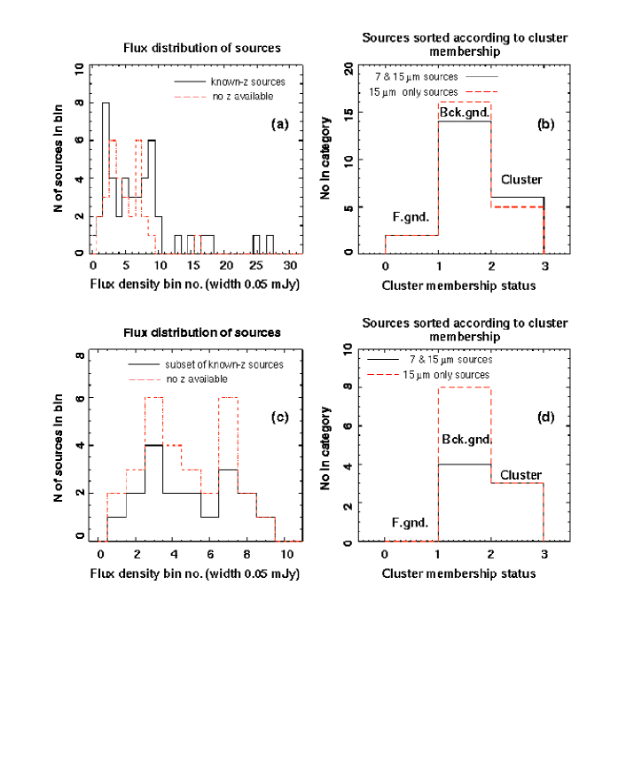
Figure 10: (a) gives, for the 15$\mu$m sample, the distribution with respect to flux-density of all sources having available redshift information (solid line), superimposed on the distribution of countable sources lacking redshift information (broken line). The known-z sample has bright outliers relative to the unknown-z sample. Nevertheless, (b) shows that between 73 and 78% of the galaxies seen at both 7 and 15 $\mu$m (solid line) or at 15 $\mu$m-only (broken line) in this sample are non-cluster galaxies (see text for further explanation). (c) gives the distributions with respect to flux-density of a subset of sources in the 15$\mu$m sample having available redshift (solid line) and yielding a flux distribution closer to the distribution of countable sources lacking redshift information (broken line). (d) shows that 75% of the galaxies seen at 15 $\mu$m-only (broken line) or 60% of galaxies seen at both 7 and 15 $\mu$m (solid line), in this sample, are non-cluster galaxies.

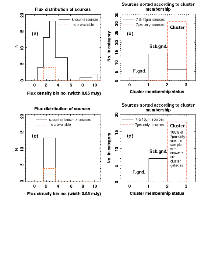
Figure 11: (a) gives, for the 7$\mu$m sample, the distribution with respect to flux-density of all sources having available redshift information (solid line), superimposed on the distribution of countable sources lacking redshift information (broken line). The known-z sample has bright outliers relative to the unknown-z sample. Nevertheless, (b) shows that 95% of the galaxies seen at 7 $\mu$m-only (broken line) are cluster members, while only 27% of galaxies seen also at 15 $\mu$m are in the clusters. (c) gives the distributions with respect to flux-density of a subset of sources in the 7$\mu$m sample having available redshift (solid line) and yielding a flux distribution closer to the distribution of countable sources lacking redshift information (broken line). (d) shows that 100% of the galaxies seen at 7 $\mu$m-only (broken line) are cluster members, while 100% of galaxies seen at both 7 and 15 $\mu$m (solid line), in this sample, are non-cluster galaxies.

6.1.2 Appropriate selection of the flux value at which to plot the counts for each bin

In order to plot the number counts reliably it is necessary to take account of the fact that the bins are quite broad and the value of the population density being sampled changes substantially across a bin. A continuous function is being sampled with a crude histogram, and so simply plotting each sample at the central flux-density of each bin results in plotted values which may fall well off the curve of the underlying population being sampled.

Assume that the population being sampled, expressed in terms of number of sources per square degree per mJy, n, is described by a power-law of the form $n=C.S^{a}$, S being the flux-density and C a constant. We sample this population by counting the number of sources dN within some flux range $S_{1}$ to $S_{2}$, and the resulting differential counts are plotted. We require that the data point for a value of the differential counts dN/dS be plotted at a flux value such that the point falls on the curve of the underlying population.

That is :

$\int_{{\Delta}S}n.dS=dN=\int_{{\Delta}S}C.S^{a}.dS=[C.S^{(a+1)}/(a+1)]_{S_{1}}^{S_{2}}$

and the differential count dN/dS should be plotted at flux-density $S_{plot}$ such that :

$dN/dS=$
$\hskip 28.45274pt[C/(a+1)].[S_{2}^{(a+1)}-S_{1}^{(a+1)}]/(S_{2}-S_{1})=C.S_{plot}^{a}$

which immediately gives the appropriate value of $S_{plot}$ for each value of the differential counts, provided one has a first-order estimate of the characteristic population index, a.

To make the differential counts plots we have derived a first-order estimate of the index by plotting the counts without any weighting, deriving a best fit slope, and then iterating. The count indices converge to the values given on the counts plots (Figs.12, 13, 14 and 15). [Obviously, in the case of the integral source counts plots showing sources per square degree down to a series of flux-density limits, the data points are always plotted at the lower end of the flux bin being integrated.]

The above approach results in Integrated Galaxy Light (IGL) totals from differential and integral counts which are mutually consistent to within a few percent. The IBL values so derived also agree well with a simple summation $\sum_{allbins}(countsperbin\times S_{plot})$. If the counts per bin are not plotted as described above to take account of bias due to the crude binning of the underlying population function, then the different methods of computing the background integral yield inconsistent results at the level of at least 20%.

6.1.3 Propagation of errors - estimation of precision

For source photometry, the flux-density uncertainty associated with each source is determined from the Monte Carlo simulations, and is the observed 1-sigma scatter in recovered flux for fake-sources of corresponding brightness inserted into the raw data cube. The scatter in recovered signal is not independent of the signal level, reflecting detailed behaviour of the reduction algorithm traced by the simulations. The noise floor for each redundancy zone of each map is determined by taking the scatter of recovered signal for the faintest fake sources recovered with at least 50% completeness. This is the noise level used to determine the significance of each detection.

We fold in quadrature the Poisson error on the number of sources detected in any given bin with a 10% uncertainty for the value of the lensing model area correction and a 10% uncertainty derived from fluctuations in the simulation completeness correction to arrive at the error estimate for counts in each counting bin.

6.1.4 Variation of area surveyed with flux - implications for cosmic variance

As described in association with Fig. 2, the area surveyed decreases as flux decreases, because the raster observation sensitivity is dependent upon position (redundancy) within the raster, and also because the amplification of the lens is dependent upon position on the sky. The mean area surveyed for the deepest bin was 2 square arcminutes in the lensing-corrected source plane, an area corresponding to a mean lensing amplification of about three and an apparent surveyed area on the sky of about 6 square arcminutes. The most sensitive 15 $\mu$m counts bin, plotted in the differential counts at 47 $\mu$Jy, relies entirely on sources from the deepest field, A2390. The second faintest 15 $\mu$m bin, plotted in the differential counts at 107 $\mu$Jy, addresses an average area of 8.2 square arcminutes in the lensing-corrected source plane and is based upon sources from the A2390 and A2218 fields. The faintest 7 $\mu$m bin reported here derives from an average area of 8.7 square arcminutes in the lensing-corrected source plane, with about equal contributions from the A2390 and A2218 fields. Overall, three cluster fields in very different directions on the sky contribute to the counts. Counts derived on a cluster by cluster basis (Metcalfe et al. 1999) were found to be consistent among the clusters.

However, it is not possible to exclude some impact of cosmic variance on the faintest 15 $\mu$m data point. Yet the clearly apparent internal consistency of the reported results (Figs.12, 13, 14 and 15), and the excellent agreement with models for the diffuse infrared background (Figs.16, 17), underline the fact that no indications have been found that we are encountering any effects of cosmic variance.

6.1.5 Source count plots

Figs.12 & 13 present respectively lensing-corrected 15 $\mu$m differential and integral source counts accumulated from the observations of the three lensing clusters.

Figs.14 & 15 present respectively lensing-corrected 7 $\mu$m differential and integral source counts accumulated from the observations of the three lensing clusters. The captions contain a detailed description of the figures.

Table 10: Number of 15 $\mu$m and 7 $\mu$m non-stellar, non-cluster, field sources falling above the 80% and 50% completeness thresholds for the survey.

Filter	Cluster	no. of	no. of
		sources	sources
		above 80%	above 50%
15 $\mu$m	A370	12	16
	A2218	23	29
	A2390	13	17
7 $\mu$m	A370	5	N/A
	A2218	11	N/A
	A2390	5	N/A

Table 11: Number of 15 $\mu$m and 7 $\mu$m countable sources per flux-density bin in the source-count plots

Filter	no. of sources above	no. of sources above
	80% compl. in bin	50% compl. in bin
	1   2    3    4    5	1    2    3    4    5
15 $\mu$m	5   10   13   10   10	9   16   15   12   10
7 $\mu$m	7   8    4 – Two sources	fell outside any used bin

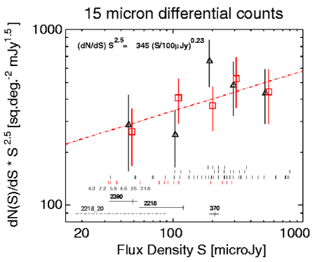
Figure 12: Lensing-corrected 15 $\mu$m differential source counts accumulated from the observations of the three lensing clusters and normalised to the Euclidean distribution. The triangles correspond to the lensing-and-completeness-corrected counts to 80% completeness. The squares represent the lensing-and-completeness-corrected counts to 50% completeness. The broken line through the data points is a simple fit to the 50% completeness data. The horizontal rows of thin vertical bars indicate the flux-densities for each of the sources used to make the counts, after correction for lensing gain. Where sources have very similar fluxes the bars have been offset vertically so that they can all be recognised. The bottom row indicates sources counted between the 50% and 80% completeness threshold. The three upper rows represent sources counted above the 80% completeness limit. The six numbers under the vertical lines list the detection significance ($\times\sigma$) for the six intrinsically weakest sources counted. (Not necessarily the apparently weakest, because of lensing.) The horizontal bars near the bottom of the plot show, for the faintest source counted in each cluster field, the apparent brightness of the source (right end of bar) and the intrinsic brightness after correction for lensing (left end). The detection limit for that cluster in the absence of lensing is indicated in each case by the intersecting vertical bar. The dashed horizontal line labelled ‘2218_20’ indicates in a similar manner the apparent and intrinsic brightness of the intrinsically faintest 15 $\mu$m source listed in the photometric tables for this survey (ISO_A2218_20).

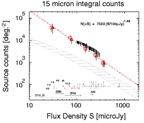
Figure 13: Lensing-corrected 15 $\mu$m integral source counts accumulated from the observations of the three lensing clusters. The triangles correspond to the lensing-and-completeness-corrected counts to 80% completeness. The squares represent the lensing-and-completeness-corrected counts to 50% completeness. The broken line through the data points is a simple fit to the data. As explained in Gruppioni et al. (2002), the hatched area represents the range of possible expectations from no–evolution models normalised to the IRAS 12 $\mu$m Local Luminosity Function (upper limit from Rush et al. 1993; lower limit from Fang et al. 1998). The black vertical hatching is the set of error bars for the HDFN counts of Elbaz et al. (1999) & Aussel et al. (1999a). Other features in the plot are as described in the caption to Fig. 12.

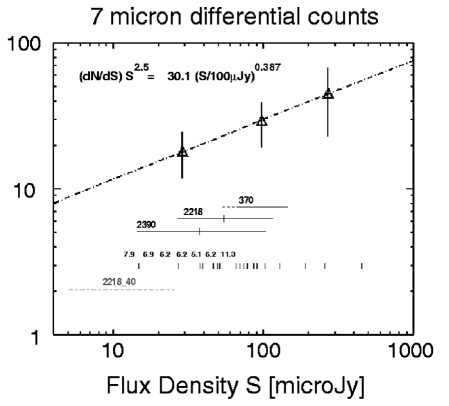
Figure 14: Lensing-corrected 7 $\mu$m differential source counts accumulated from the observations of the three lensing clusters and normalised to the Euclidean distribution. The triangles correspond to the lensing and completeness corrected counts to 80% completeness. Other features in the plot are as described in the caption to Fig. 12, but the dashed horizontal line labelled ‘2218_40’ indicates (in the manner described for Fig. 12) the apparent and intrinsic brightness of the intrinsically faintest 7 $\mu$m source listed in the photometric tables for this survey (ISO_A2218_40).

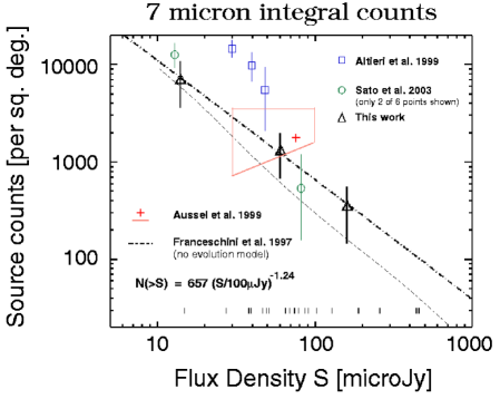
Figure 15: Lensing-corrected 7 $\mu$m integral source counts accumulated from the observations of the three lensing clusters. The triangles correspond to the lensing and completeness corrected counts to 80% completeness. The broken line through the data points is a simple fit to the data. The low dashed line corresponds to the no-evolution model of Franceschini et al. (1997). The polyhedron containing the (+) symbol indicates the 1-sigma error-box and best estimate 7 $\mu$m counts value of Aussel et al. (1999a), based on Hubble Deep Field observations. The circles and squares are as indicated on the plot. Other features in the plot are as described in the captions to Fig. 12 and Fig. 14.

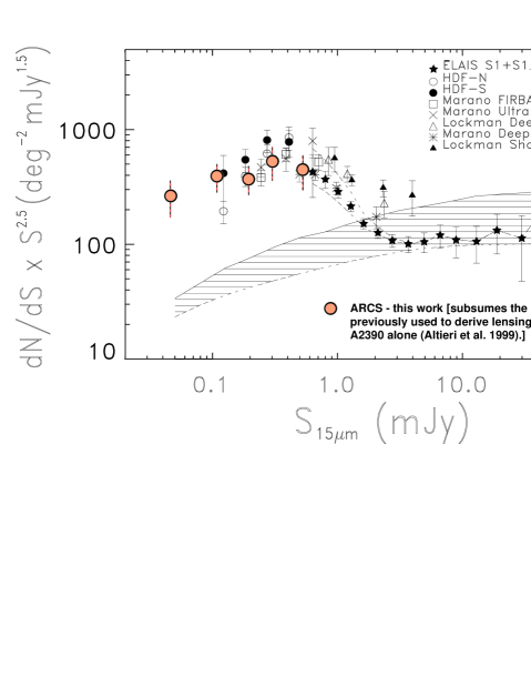
Figure 16: Adapted from Gruppioni et al. (2002) figure 8. Differential source counts at 15 $\mu$m normalised to the Euclidean distribution ($dN/dS\propto S^{-2.5}$). The results from various ISO surveys are shown in the figure, including the present lensing survey, which extends the plot to fainter sources. As explained in Gruppioni et al. (2002), the hatched area represents the range of possible expectations from no–evolution models normalised to the IRAS 12 $\mu$m Local Luminosity Function (upper limit from Rush et al. (1993); lower limit from Fang et al. (1998)).

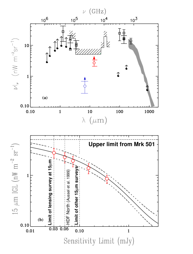
Figure 17: This figure is adapted from figs.3 and 10 of Elbaz et al. (2002). (a) presents limits to, and measurements of, the Integrated Galaxy Light (IGL, filled dots) and Extragalactic Background Light (EBL, open squares, grey area) from the UV to sub-millimeter, as described in the Elbaz et al. (2002) figure 10. EBL measurements from COBE: 200-1500 $\mu$m EBL from COBE-FIRAS (grey area, Lagache et al. 1999), 1.25, 2.2, 3.5, 100, 140 $\mu$m EBL from COBE-DIRBE (open squares). IGL in the U,B,V,I,J,H,K bands from Madau & Pozzetti (2000). The upper end of the arrows indicate the revised values suggested by Bernstein et al. (2002, a factor of two higher). The hatched upper limit at 5 $\times 10^{-9}$ Wm^-2 sr^-1 is obtained from the absorption of TeV photons with the extragalactic infrared background. We have concatenated our 15 $\mu$m counts with higher flux data from the Elbaz et al. paper to arrive at a deeper and so higher value of the 15 $\mu$m IGL, (2.7$\pm$0.62)$\times$10^-9 W m^-2 sr^-1. We have replaced the Altieri et al. (1999) value for the 7 $\mu$m integral which Elbaz et al. (2002) plotted with the revised value (0.49$\pm$0.2)$\times$10^-9 W m^-2 sr^-1. (b) shows values of the integral over the 15 $\mu$m source counts evaluated to various flux limits and plotted over the Elbaz et al. (2002) Fig.3 fit to the counts of other ISOCAM deep surveys. Our data points extend the flux-limit of the observations and remain consistent with the fit. The dashed lines correspond to 1-$\sigma$ error bars obtained by Elbaz et al. (2002) fitting the upper and lower limits of the source counts from other surveys. The error bars on our overplotted data points are obtained by integrating over the upper and lower limits of the differential counts values.

7 Discussion

7.1 Source counts and Log N-Log S distributions

Several independent field surveys were conducted in the mid-infrared using ISOCAM (e.g. Rowan-Robinson et al., 1997; Taniguchi et al., 1997; Altieri et al., 1999; Aussel et al., 1999a; Elbaz et al., 1999 & 2000; Serjeant et al., 2000; Oliver et al., 2000; Lari et al., 2001; Gruppioni et al., 2002; Sato et al., 2003). Many of their results have been summarised in Elbaz et al. (1999 & 2002). The Elbaz et al. (1999) paper includes all counts from the Lockman Hole, Marano Field, HDFN, HDFS and the results of our earlier work on A2390 (Altieri et al. 1999).

Fig. 16, adapted from figure 8 of Gruppioni et al. (2002), compares the 15 $\mu$m differential source counts from this work with corresponding results from various ISO surveys, as identified in the figure. The 15 $\mu$m lensing corrected source counts from the three clusters presented here are in excellent agreement with the other surveys where the flux ranges overlap. (The A2390 lensing points from Altieri et al. (1999) which appear in the figure in Lari et al. are here revised and subsumed in our global analysis of the three lensing clusters.)

Extending, and confirming, the results of the earlier surveys, the 15 $\mu$m counts in Fig. 12 & Fig. 13 show a steadily increasing excess by a factor of order 10 over no-evolution models (see references in figure captions). The slope of the 15 $\mu$m differential counts is -2.28 down to the 30 $\mu$Jy limit. These source densities favour extreme evolution models. The mid-infrared-luminous galaxies have been interpreted (Aussel et al. 1999b; Elbaz et al. 1999 & 2000; Serjeant et al. 2000) as a population of dust-enshrouded star forming galaxies. Within the current detection limits, they have a median redshift of about 0.8 over all CAM deep surveys (Elbaz et al. 2002). The median z of all field (non-cluster) galaxies in the present work is 0.6, with a value of 0.65 applying to the background lensed sources. We attribute the difference between the Elbaz-quoted value and the value from this work to two possible sources: (a) spectroscopic redshift values were not available for all counted sources. For sources lacking spectroscopic redshift values we inferred that they are non-cluster sources based on strong IR colour rules derived on the known redshift set (see Sec.6.1.1. It seems reasonable to suggest that the sources lacking spectroscopic redshift values will be the optically fainter, therefore more distant, sources. Now we determined our median value from the set of sources for which we have spectroscopic z values. Therefore our median redshift estimate is likely to be biased towards lower redshift. (b) As discussed in Sec.6.1.4, we cannot rule out some impact of cosmic variance on our results, due to the limited field areas surveyed.

As pointed out in Elbaz et al. (2002), the 15 $\mu$m number counts cannot be explained without invoking either a strong evolution of the whole luminosity function (Xu 2000, Chary & Elbaz 2001) or preferentially of a sub-population of starburst galaxies evolving both in luminos-

ity and density (Franceschini et al. 2001, Chary & Elbaz 2001, Xu et al. 2001).

The evidence for strong evolution does not show up so clearly in the 7 $\mu$m counts (Fig. 14 & Fig. 15) which, within the error bars, are consistent with the Franceschini et al. (1997) no-evolution model. This is not surprising, because the powerful starbursts associated with strong evolution are hidden in the optical and near-infrared by absorbing clouds of dust. They become apparent through the reprocessing of the starburst radiation into Unidentified Infrared Band (UIB) dust emission. (For a local example see Vigroux et al. 1996; Mirabel et al. 1998). For the redshift range of the observed mid-infrared population, i.e. beyond z=0.4, the 7 $\mu$m filter bandpass band is no longer sensitive to the UIB emission, but is dominated by redshifted stellar light from the rest-frame near-IR. On the other hand, at similar redshifts the UIB emission associated with dust absorbed starburst emission has been redshifted into the 15 $\mu$m band, and falls in that band for redshift values up to $\sim$2.

The redshift range of the 7 $\mu$m known-z non-cluster field sources is 0.026 to 2.8, with a median value of 0.55. The slope of the 7 $\mu$m differential counts is -2.11 down to the 14 $\mu$Jy limit. It is important to note that, of the 20 sources used to derive the three 7 $\mu$m data points in Figs.14 & 15, fourteen have spectroscopic redshifts, one is morphologically an obvious foreground elliptical (ISO_A370_07+), three (ISO_A2218_17, _51, and _67) have been securely identified as galaxies based on SED modelling (Biviano, private communication), one (ISO_A2218_61a) has been classified morphologically (as S0) from HST images by Smail et al. (2001), and one (ISO_A2390_22) has galactic, not stellar, mid-infrared colour. So our 7 $\mu$m counts are not at all contaminated by stars, nor are they contaminated by cluster galaxies (see Sec.6.1.1, above).

7.2 Extragalactic Infrared Background

The population of mid-infrared bright galaxies observed by ISOCAM at 15 $\mu$m can account for the bulk of the Cosmic Infrared Background (CIRB), so that a large fraction of stars seen today must have formed in dusty starbursts, such as those affecting the ISOCAM galaxies (Elbaz et al.  2002, Lari et al, 2001, Altieri et al. 1999). It is interesting that Elbaz et al. (2002) also remark that the unlensed ISOCAM and SCUBA surveys do not sample the same redshift and luminosity ranges, and hence show virtually no overlap (Hughes et al. 1998), but that greater overlap of the samples is expected in the deeper, lensed, cases. Indeed we find that from a sample of 15 SCUBA sources reported in the three clusters discussed in this paper (Ivison et al. 1998; Smail et al. 2002; Cowie et al. 2002) seven are seen in our ISOCAM 15 $\mu$m sample. [I.e. sources ISO_A370_09, ISO_A370_17, ISO_A2390_43, ISO_A2390_37 (cD galaxy), ISO_A2390_19, ISO_A2390_28a and ISO_A2390_42]. We will discuss these cases in more detail in a later paper.

We concatenate the source counts obtained from the sample of lensed background sources (and the few foreground sources) to the extensive results of the other ISOCAM field surveys reported by Elbaz et al. (2002). Integrating in the achieved flux density range from 30$\mu$Jy to 50 mJy, we resolve (2.7$\pm$0.62)$\times$10^-9 W m^-2 sr^-1 of the 15 $\mu$m infrared background into discrete sources. We similarly have resolved a significant fraction of the 7 $\mu$m diffuse infrared background, finding a lower value than reported in Altieri et al. (1999), but agreeing well with the 7 $\mu$m counts of Sato et al. (2003) recorded on the SSA13 field. The 7 $\mu$m integral relies entirely on the lensing counts in the limited flux-density range from 14 $\mu$Jy and 460 $\mu$Jy to resolve (0.49$\pm$0.2)$\times$10^-9 W m^-2 sr^-1, or $\sim$10%, of the 7 $\mu$m infrared background. In all cases the error limits are 1$\sigma$ values.

We attribute the lower values found here for the IGL integrals, relative to the Altieri et al. (1999) value, to a much more thorough rejection of cluster galaxy contamination (in the 7 $\mu$m case), and generally, to a much more rigourous Monte Carlo analysis of the completeness threshold performed in this work over the several intervening years.

Fig. 17(a) and (b) are adapted from figures 10 and 3, respectively, of Elbaz et al. (2002). (a) gives current limits to, and measurements of, the background radiation from UV to sub-millimetre wavelengths, as described in Elbaz et al. (2002) figure 10. The two mid-infrared points take into account the results of the work reported here, placed into the context of all the ISOCAM surveys. The 15 $\mu$m resolved Intergalactic Light (IGL) integral benefits from the results of shallower surveys to reach deeper, and so higher, integral values which are, as can be seen in Fig. 17(b), consistent with the fit derived by Elbaz et al. (2002), but extending to fainter flux-densities the experimental confirmation of their fit.

The spectra of high energy gamma-ray sources are predicted to be modified by absorption effects caused by the pair-production interaction of the gamma-rays with the extragalactic background light (EBL) (Stecker, de Jager and Salamon 1992). The peak absorption occurs at wavelengths of $\lambda(\mu m)$ = 1.24 $E_{\gamma}(TeV)$ and infrared photons are very effective at attenuating gamma-rays of energies $E_{\gamma}\sim$ 1-100 TeV (see Hauser and Dwek 2001 for a recent review). The probing of the infrared background has recently become practical with a range of gamma-ray observatories and observations that have recently been reviewed by Catanese and Weekes (2002). The spectra of the high energy gamma rays from Mkn 421 and 501 have been used to place an upper limit of 5.0 $\times 10^{-9}$ Wm^-2 sr^-1 on the infrared background around 15 $\mu$m, as shown by the hatched region in Fig 17(a) (Aharonian et al. 1999; de Jager and Stecker 2002; Stanev and Franceschini 1997; Malkan and Stecker 2001; Renault et al. 2001; Hauser and Dwek 2001). The contribution reported here to the infrared background light is 55% of the upper limit and most of the infrared background is now resolved into discrete sources (Figs. 17(a) and (b)).

However the recent detections of TeV gamma rays (Horan et al. 2002: Petry et al. 2002: Aharonian et al. 2002) from the BL Lac H1426+428 at z = 0.129, well beyond the redshifts of Mkn 421 (z=0.03) and Mkn 501 (z=0.034), imply severe absorption of TeV photons by the optical and infrared backgrounds. The value of the 15 $\mu$m background presented here has important consequences for the TeV emission from H1426+428 because it implies a factor of 20 attenuation for the TeV photons, additional to the factor for Mkn 501. It is now reasonable to expect that further observations of TeV gamma ray blazars will determine both the optical and infrared extragalactic backgrounds (Aharonian et al. 2002; Weekes et al. 2002).

7.3 Star formation history

We take the opportunity to underline here the particular importance of the ISOCAM mid-infrared observations in constraining important aspects of the global history of star formation (Elbaz et al. 2002). The Madau plot underestimates the star formation rate density per comoving volume in the universe because in the first version (Madau et al. 1996) no correction for extinction was included, and in subsequent work (Madau et al. 1999) and other studies (e.g. Adelberger & Steidel, 2000; Meurer et al. 1999) the extinction correction is done assuming the Calzetti law (Calzetti 1997) or the beta-slope technique from Meurer et al. (1999). These techniques used to correct for extinction also underestimate the true star formation rate which is measured in the mid and far IR, as shown in the more recent paper by Goldader et al. (2002) (see their Fig.1).

Luminous infrared galaxies appear to play a major role in the star formation events that took place during the last 8-10 Gyr (since z$\sim$1-1.2), as shown by the survey results already discussed and their interpretation in terms of contribution to the star formation history and cosmic infrared background (Elbaz et al. 2002; Chary & Elbaz 2001). The initial Madau plot, from rest-frame UV data, was missing two thirds of the star formation activity in galaxies, and correcting for extinction with the UV-slope technique, as done by several authors, still misses most of it, since this law does not work for luminous IR galaxies (see Goldader et al. 2002, Fig.1).

8 Conclusions

In this paper, we have described the use of the ISOCAM camera on board ESA’s Infrared Space Observatory mission to employ clusters of galaxies as natural lenses to extend the mid-Infrared source counts of field sources to the deepest levels, at both 7 $\mu$m and 15 $\mu$m. A flux selected subset of the sources above the 80% and 50% completeness limits was used to derive cumulative source counts to a lensing corrected sensitivity level of 30 $\mu$Jy at 15 $\mu$m, and 14 $\mu$Jy at 7 $\mu$m. For the 7 $\mu$m bandpass cluster sources were numerous, but cluster contamination could be eliminated by reference to source spectroscopic redshift, and in a few cases by the strong correlation between mid-IR colour and cluster membership. The 15 $\mu$m source counts, corrected for the effects of contamination by cluster sources and lensing, confirm and extend earlier findings of an excess by a factor of 10 with respect to source models with no evolution.

We resolve (2.7$\pm$0.62)$\times$10^-9 W m^-2 sr^-1 of the 15 $\mu$m infrared background into discrete sources by integrating over our source counts, concatenated to those from other extensive ISOCAM surveys, in the flux range from 30$\mu$Jy to 50 mJy. We resolve (0.49$\pm$0.2)$\times$10^-9 W m^-2 sr^-1 of the 7 $\mu$m infrared background into discrete sources by integrating over our source counts in the flux range from 14 $\mu$Jy to 460 $\mu$Jy.

Recent detections of TeV gamma rays from more distant BL Lac sources serve to underline the opacity, to TeV photons, of the mid-infrared photon densities reported in this work and give reason to suspect that the mid-infrared flux-densities found may indeed account for a larger fraction of the diffuse background than the 55% mentioned just above in the discussion.

These results suggest that abundant star formation occurs in very dusty environments at z$\sim$1. The next Mid-Infrared (SIRTF, NGST) and Far-Infrared (Herschel) mission, will clearly help in understanding star-formation processes at high redshift.

We have demonstrated over an unprecedentedly large source sample that gravitational lens models for galaxy clusters can be successfully used to perform statistical source-counting surveys to depths otherwise unachievable with the same instrumentation. We have presented a photometric catalogue of 145 mid-infrared sources to unprecedented depth, containing roughly 15% of all deep survey sources detected in the several extensive ISOCAM surveys.

When deep cosmological surveys are planned for future missions, the use of nature’s own telescopes to increase the depth of the surveys should not be considered as a novelty. It should form an indispensible part of the core survey strategy from the outset. The potential of this technique has only been illustrated in this work, which has drawn upon what has probably been close to the minimum viable dataset for these purposes. The more clusters used in a lensing survey the more area is accumulated at the highest amplification values. As the plots in Fig. 2 illustrate, lensing has the potential to make sources available at intrinsic fluxes arbitarily fainter than the apparent flux limit for deep blank–field surveys made with the same instrumentation.