How magnetic helicity ejection helps large scale dynamos

Abstract

There is mounting evidence that the ejection of magnetic helicity from the solar surface is important for the solar dynamo. Observations suggest that in the northern hemisphere the magnetic helicity flux is negative. We propose that this magnetic helicity flux is mostly due to small scale magnetic fields; in contrast to the more systematic large scale field of the 11 year cycle, whose helicity flux may be of opposite sign, and may be excluded from the observational interpretation. Using idealized simulations of MHD turbulence as well as a simple two-scale model, we show that shedding small scale (helical) field has two important effects. (i) The strength of the large scale field reaches the observed levels. (ii) The evolution of the large scale field proceeds on time scales shorter than the resistive time scale, as would otherwise be enforced by magnetic helicity conservation. In other words, the losses ensure that the solar dynamo is always in the near-kinematic regime. This requires, however, that the ratio of small scale to large scale losses cannot be too small, for otherwise the large scale field in the near-kinematic regime will not reach the observed values.

INTRODUCTION

In recent years a new term has entered the solar physics vocabulary: magnetic helicity. This topic has received significant attention on two quite different fronts that now seem to converge in their mutual importance. The detection of helical features has received interest firstly as a purely diagnostic tool to characterize topological complexity. As magnetic helicity is a conserved quantity (neglecting boundary losses and resistivity), this has secondly been seen to impose constraints on mean-field dynamo theory; with the advent of powerful massively parallel computers, these constraints are now also being confirmed numerically as progressively larger magnetic Reynolds numbers are becoming possible.

In the following we discuss briefly the observational aspects relevant to the dynamo problem and turn then to the connection with dynamo theory. We then present arguments linking the loss of small scale (SS) field to an enhancement of the large scale (LS) dynamo.

THE OBSERVED LARGE SCALE FIELD

The question of scales is very important: what is large scale to an observer could be small scale to a dynamo theorist, for example. Looking at the magnetic field in helmet streamers reveals structures comparable to the solar radius, which might be taken to belong to the large scale field. This may be misleading, however. For a dynamo theorist who wants to explain the 11 year solar cycle it matters that there are bipolar regions with systematic orientation and tilt, but longitudinal departures from the mean axisymmetric form are secondary to the underlying effect that sustains the field. Longitudinal averages are therefore a sensible tool to extract what a dynamo theorist might want to call large scale field.

That such a definition makes some sense can be seen by looking at longitudinally averaged magnetograms of the solar surface as a function of latitude and time. We reconstruct such a space-time diagram from the amplitude and phase coefficients, $\hat{B}_{\ell}$ and $\phi_{\ell}$ respectively, given by Stenflo (1988). Following earlier work (Stenflo & Vogel 1986, Stenflo & Güdel 1988) he described the radial component of the longitudinally averaged field of dipole symmetry in the form

$$\overline{B}_{r}(\theta,t)=\sum_{\ell=1,3,...}\hat{B}_{\ell}P_{\ell}(\cos\theta)\,\cos[\omega(t-t_{0})+\phi_{\ell}],$$ (1)

where $P_{\ell}$ is the Legendre polynomial and $\omega=2\pi/22{\rm years}$ is the cycle frequency; the values of $\hat{B}_{\ell}$ and $\phi_{\ell}$ are reproduced in Table 1.

Table 1: Phase and amplitude coefficients describing the mean dipole symmetry radial field at the solar surface, from Stenflo (1988). The last row gives the contributions to the root-mean-square value of the field, $\hat{B}_{\ell}/\sqrt{2(2\ell+1)}$. The phase is defined relative to the epoch $t_{0}=1960\,{\rm yr}$.

$\ell$ 1 3 5 7 9 11 13 $\phi_{\ell}/2\pi$ 0.24 0.29 1.07 1.59 1.95 2.45 2.85 $\hat{B}_{\ell}\,\mbox{[gauss]}$ 1.49 1.66 3.15 2.28 2.64 1.56 0.92 $\hat{B}_{\ell}/\sqrt{2(2\ell+1)}\,\mbox{[gauss]}$ 0.61 0.44 0.67 0.42 0.43 0.23  0.12

Since the mean field is (by definition) axisymmetric, its poloidal part can be written in the form $\overline{\mbox{\boldmath$B$}}_{\rm pol}=\mbox{\boldmath$\nabla$}{}\times(\overline{A}_{\phi}\hat{\mbox{\boldmath$\phi$}}{})$. This allows us to relate the surface values of $\overline{B}_{r}$ to $\overline{A}_{\phi}$,

$$\overline{B}_{r}={1\over r\sin\theta}\,{\partial\over\partial\theta}\,\left(\sin\theta\overline{A}_{\phi}\right),\quad r=R_{\odot}.$$ (2)

Note that no radial derivatives enter, so that we can obtain $\overline{A}_{\phi}$ by surface integration. To express $\overline{A}_{\phi}$ more simply, note that we can also write $\overline{\mbox{\boldmath$B$}}_{\rm pol}$ in terms of the poloidal potential $\overline{S}$, i.e.

$$r\overline{B}_{r}=\mbox{\boldmath$r$}{}\cdot\mbox{\boldmath$\nabla$}{}\times\mbox{\boldmath$\nabla$}{}\times(\overline{S}\mbox{\boldmath$r$}{})\equiv-L^{2}\overline{S},$$ (3)

where $L^{2}$ is the angular part of the Laplacian, in spectral space satisfying $-L^{2}=\ell(\ell+1)$. Since $\overline{A}_{\phi}=-\partial\overline{S}/\partial\theta$ and $\partial P_{\ell}/\partial\theta=P_{\ell}^{1}$, we have

$$\overline{A}_{\phi}(\theta,t)=-\sum_{\ell=1,3,...}{r\over\ell(\ell+1)}\hat{B}_{\ell}P_{\ell}^{1}(\cos\theta)\,\cos[\omega(t-t_{0})+\phi_{\ell}].$$ (4)

In Figure 1 we show both $\overline{B}_{r}$ and $\overline{A}_{\phi}$, as reconstructed using equations (1) and (4).

Fig. 1: Mean dipole symmetry radial field, $\overline{B}_{r}$, reconstructed from the coefficients of Stenflo, 1988 (upper panel). The corresponding toroidal component of the mean vector potential, $\overline{A}_{\phi}$, derived from $\overline{B}_{r}$ (lower panel). Solid contours denote positive values, dotted contours negative values. The solar cycle maximum of 1981 is highlighted, as is the latitude of 10^∘ where $\overline{B}_{r}$ was then strongest. The signs of various quantities at or around this epoch are also shown (see text for more details).

Stenflo’s coefficients suggest that the sun’s large scale magnetic field is dominated by the higher harmonics around $\ell=5$. The coefficient of the basic dipole mode, $\hat{B}_{1}$, is only the sixth-largest among all coefficients. This misrepresents the energy present in the various modes, however. The integral of $\overline{B}_{r}^{2}$ over the full surface and over one cycle divided by the surface area and the length of the cycle is equal to the sum of $\hat{B}_{\ell}^{2}/[2(2\ell+1)]$. In Table 1 its square root, i.e. the contribution to the rms field strength, is given. Although the contribution from $\ell=5$ is still the largest, the basic dipole contribution is now the second largest. In that sense one is justified in talking of the Sun’s field as dipolar.

The magnetic helicity of the large scale field, as defined above, is an important quantity. Magnetic helicity, $\int\overline{\mbox{\boldmath$A$}}\cdot\overline{\mbox{\boldmath$B$}}\,{\rm d}{}V$, can be tricky to work with, since it involves the magnetic vector potential, $\overline{\mbox{\boldmath$A$}}$ (with $\overline{\mbox{\boldmath$B$}}=\mbox{\boldmath$\nabla$}{}\times\overline{\mbox{\boldmath$A$}}$), which is not directly observable. Attempts to reconstruct $\overline{\mbox{\boldmath$A$}}$ from $\overline{\mbox{\boldmath$B$}}$ raise the question of the choice of a gauge; and the magnetic helicity is not in general gauge invariant. This problem can be avoided by considering instead the gauge invariant magnetic helicity of Berger & Field (1984),

$$H=\int_{V}(\overline{\mbox{\boldmath$A$}}+\overline{\mbox{\boldmath$A$}}_{\rm P})\cdot(\overline{\mbox{\boldmath$B$}}-\overline{\mbox{\boldmath$B$}}_{\rm P})\;{\rm d}{}V,$$ (5)

where $\overline{\mbox{\boldmath$B$}}_{\rm P}=\mbox{\boldmath$\nabla$}{}\times\overline{\mbox{\boldmath$A$}}_{\rm P}$ is a potential reference field inside $V$ with the boundary condition $\mbox{\boldmath$r$}{}\cdot\overline{\mbox{\boldmath$B$}}_{\rm P}=\mbox{\boldmath$r$}{}\cdot\overline{\mbox{\boldmath$B$}}$. As shown in Brandenburg, Dobler & Subramanian (2002), for an axisymmetric mean field expressed as $\overline{\mbox{\boldmath$B$}}=\overline{B}_{\phi}\hat{\mbox{\boldmath$\phi$}}{}+\mbox{\boldmath$\nabla$}{}\times(\overline{A}_{\phi}\hat{\mbox{\boldmath$\phi$}}{})$, with $\overline{A}_{\phi}=\overline{B}_{\phi}=0$ on the axis, this yields simply

$$H=2\int_{V}\overline{A}_{\phi}\overline{B}_{\phi}\;{\rm d}{}V.$$ (6)

There is no way to determine this quantity for the sun without knowing both $\overline{A}_{\phi}$ and $\overline{B}_{\phi}$ throughout the entire sphere. Experience with axisymmetric mean field dynamos shows, however, that the product $\overline{A}_{\phi}\overline{B}_{\phi}$ does not vary strongly in radius, so considering this quantity at the surface may still be useful.

The question of the sign of $\overline{A}_{\phi}\overline{B}_{\phi}$ is related to the question of the phase relation between toroidal and poloidal field, which was investigated in the mid seventies (Stix 1976a,b, Yoshimura 1976). By estimating the phase shift between $\overline{B}_{r}$ and $\overline{B}_{\phi}$, it was argued that the radial angular velocity gradient, $\partial\Omega/\partial r$, should be negative. This, together with the fact that the solar dynamo wave propagates equatorward, suggested that $\alpha$ is positive (negative) in the northern (southern) hemisphere. Our knowledge has changed since then: (i) we now know from helioseismology that $\partial\Omega/\partial r$ is positive (suggesting that something may be wrong with the observed phase relation); (ii) the direction of propagation of the dynamo wave can be reversed by meridional circulation (Durney 1995, Choudhuri, Schüssler & Dikpati 1995). The question of the sign of $\overline{A}_{\phi}\overline{B}_{\phi}$ differs somewhat from that of the phase relation; the former should depend on the sign of $\alpha$, not on the sign of $\partial\Omega/\partial r$. Let us ignore for a moment the problems with the traditional phase relation then, and discuss what can be said about the sign of $\overline{A}_{\phi}\overline{B}_{\phi}$ at the surface.

Yoshimura (1976) estimated the magnitude of the toroidal field by averaging the unsigned surface flux in an appropriate fashion. The idea is that the toroidal field emerges as $\Omega$-loops at the surface, and that a stronger toroidal field shows up as an increased level of unsigned flux, i.e. $|\overline{B}_{\phi}|\propto\overline{|B_{r}|}$ (note that the modulus is underneath the average of $B_{r}$). He then determined the sign of $\overline{B}_{\phi}$ simply by looking at the orientation of the bipolar regions on solar magnetograms. This tells us that during the maximum of Cycle 21 in 1981 or 1982 the toroidal field was negative (positive) in the northern (southern) hemisphere. Comparing with $\overline{B}_{r}$ of Figure 1 (upper panel) we see that $\overline{B}_{r}$ was positive (solid contours at 10^∘; here we focus on latitudes near the equator where $\overline{B}_{r}$ is strongest); hence $\overline{B}_{r}\overline{B}_{\phi}$ was negative. This verifies the original finding of Stix (1976a) and Yoshimura (1976). Comparing with $\overline{A}_{\phi}$ of Figure 1 (lower panel), the situation is less clear; $\overline{A}_{\phi}\overline{B}_{\phi}$ may be negative just before solar maximum and positive just after solar maximum. This suggests that the gauge invariant magnetic helicity $H$ (given by equation (6)) might be close to zero. This analysis clearly requires more complete data for $\overline{B}_{\phi}$, however. Given that a much longer data record is now available, it is surprising that the analysis of Yoshimura (1976) has never been repeated; better constraints on this quantity would be very useful.

In the following we emphasize the importance of determining the sign of the magnetic helicity of the LS field and we suggest that, on theoretical grounds, its sign should be opposite to that of the SS field. We know that in active regions the magnetic helicity is negative (positive) in the northern (southern) hemisphere (Seehafer 1990, Pevtsov, Canfield & Metcalf 1995, Bao et al. 1999, Démoulin et al. 2002). We use this to support our expectation that what is observed in active regions is actually the helicity of the SS field.

1 RELATIONSHIP BETWEEN LARGE AND SMALL SCALE FIELDS

Kinematic theory is able to explain the growth of helical fields at large scales (LS) and the growth of helical and non-helical fields at small scales (SS). The growth rate of the SS field is usually much larger than that of the LS field, and it was therefore thought that the rapid growth of this SS fields tends to suppress the growth of the LS field (Kulsrud & Anderson 1992), and that the solar magnetic field may therefore be of primordial origin (Vainshtein & Cattaneo 1992). This seemed however to be in conflict with several successful numerical simulations of large scale dynamo action that showed the SS field to be merely comparable in strength to the LS field (Glatzmaier & Roberts 1995, Brandenburg et al. 1995, Brandenburg 2001).

Meanwhile it has become clear that it is not the SS field as such that causes problems, but only the helical part of the SS field that is generated simultaneously with the LS field. This phenomenon has been seen in simulations of MHD turbulence with helical forcing (Brandenburg 2001) and has been modeled successfully with semi-analytic, nonlinear two-scale theories (Field & Blackman 2002; Blackman & Brandenburg 2002; Blackman & Field 2002). These approaches assume (perhaps correctly) that the dynamo works primarily via helicity-dependent effects, by which we mean both the $\alpha$-effect (Steenbeck, Krause, Rädler 1966) or the inverse cascade/transfer (Pouquet, Frisch & Léorat 1976). Some alternatives have been proposed: the Vishniac-Cho (2001) effect (but see Arlt & Brandenburg 2001) and negative turbulent magnetic diffusivity (Zheligovsky, Podvigina & Frisch 2001).

The essence of the nonlinearity of helical dynamos is that the helicity effects produce large scale helical magnetic fields, but the total magnetic helicity is conserved, so there must be a simultaneous generation of magnetic fields of opposite helicity. Splitting the field into LS and SS components, $\mbox{\boldmath$B$}{}=\overline{\mbox{\boldmath$B$}}+\mbox{\boldmath$b$}{}$, and likewise for the magnetic vector potential, $\mbox{\boldmath$A$}{}=\overline{\mbox{\boldmath$A$}}+\mbox{\boldmath$a$}{}$, we have to satisfy

$$\langle\mbox{\boldmath$A$}{}\cdot\mbox{\boldmath$B$}{}\rangle=\langle\overline{\mbox{\boldmath$A$}}\cdot\overline{\mbox{\boldmath$B$}}\rangle+\langle\mbox{\boldmath$a$}{}\cdot\mbox{\boldmath$b$}{}\rangle\approx 0.$$ (7)

If the LS field were fully helical, and of typical wavenumber $k_{\rm m}$, we would have $k_{\rm m}\langle\overline{\mbox{\boldmath$A$}}\cdot\overline{\mbox{\boldmath$B$}}\rangle=\pm\langle\overline{\mbox{\boldmath$B$}}^{2}\rangle$, depending on the sign of the magnetic helicity of the LS field. For fractional helicity of the forcing one has instead

$$k_{\rm m}\langle\overline{\mbox{\boldmath$A$}}\cdot\overline{\mbox{\boldmath$B$}}\rangle=\epsilon_{\rm m}\langle\overline{\mbox{\boldmath$B$}}^{2}\rangle,$$ (8)

where $|\epsilon_{\rm m}|\leq 1$, and $\epsilon_{\rm m}=0$ for non-helical fields. A similar relation applies to the fluctuating field (of wavenumber $k_{\rm f}$) and its helicity, i.e. $k_{\rm f}\langle\mbox{\boldmath$a$}{}\cdot\mbox{\boldmath$b$}{}\rangle=\epsilon_{\rm f}\langle\mbox{\boldmath$b$}{}^{2}\rangle$. With these preliminaries we can say that in a magnetic helicity conserving situation

$${\langle\overline{\mbox{\boldmath$B$}}^{2}\rangle\over\langle\mbox{\boldmath$b$}{}^{2}\rangle}={k_{\rm m}\over k_{\rm f}}\,{\epsilon_{\rm f}\over\epsilon_{\rm m}}.$$ (9)

If $|\epsilon_{\rm f}|\approx|\epsilon_{\rm m}|$, and since $k_{\rm m}<k_{\rm f}$ for finite scale separation, we have in this phase $\langle\overline{\mbox{\boldmath$B$}}^{2}\rangle<\langle\mbox{\boldmath$b$}{}^{2}\rangle$. We note, however, that in $\alpha\Omega$ dynamos where a strong toroidal LS field can be generated from a poloidal LS field, regardless of helicity — so that $k_{\rm m}\langle\overline{\mbox{\boldmath$B$}}^{2}\rangle\gg|\langle\overline{\mbox{\boldmath$J$}}\cdot\overline{\mbox{\boldmath$B$}}\rangle|$ — one may have $|\epsilon_{\rm m}|\ll|\epsilon_{\rm f}|$. It is then possible that $\langle\overline{\mbox{\boldmath$B$}}^{2}\rangle$ can be comparable to or in excess of $\langle\mbox{\boldmath$b$}{}^{2}\rangle$, or at least it helical component (Blackman & Brandenburg 2002).

To summarize, magnetic helicity conservation links the magnitude of the helical components of the LS and SS fields in a well defined way, depending mainly on the degrees to which LS and SS fields are helical, i.e. on the values of $\epsilon_{\rm m}$ and $\epsilon_{\rm f}$. For simple dynamos in slab geometry these values can be determined from kinematic theory (Blackman & Brandenburg 2002).

SIMULTANEOUS PRODUCTION OF LARGE AND SMALL SCALE TWIST

Given that magnetic helicity is conserved in the absence of boundary losses and resistivity, any swirl-like motion must simultaneously introduce oppositely helical magnetic fields when starting with an initially non-helical magnetic field (Longcope & Klapper 1997). The prime example is of course the formation of an $\Omega$-shaped flux loop due to magnetic or thermal buoyancy, and the simultaneous tilting due to the Coriolis force. This is sketched in Fig. 2.

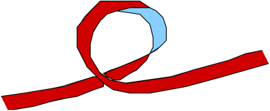
Fig. 2: Tilting of the rising tube due to the Coriolis force. Note that the tilting of the rising loop causes also internal twist.

Fig. 3: Magnetic helicity spectra (scaled by wavenumber $k$ to give magnetic helicity per logarithmic interval) taken over the entire computational domain. The spectrum is dominated by a positive component at large scales ($k=1-5$) and a negative component at small scales ($k>5$).

We consider now the result of a simulation of a buoyant magnetic flux tube. Similar calculations have been carried out many times in the past (e.g. Abbett, Fisher & Fan 2000), but here we are interested in the magnetic helicity spectrum, which seems to have attracted little attention so far. We start with a horizontal flux tube in the azimuthal ($y$-) direction with vanishing net flux (so there is a weak oppositely oriented field outside the tube) and a $y$-dependent sinusoidal modulation of the entropy along the tube. This destabilizes the tube such that it rises in one portion of the box. Although the box is not periodic in the vertical direction, the boundary conditions are still sufficiently far away that we can obtain power spectra of the magnetic helicity via Fourier transforms; see Fig. 3. Note that after some time ($t=6$ free-fall times) the spectrum begins to show mostly positive magnetic helicity (as expected), together with a gradually increasing higher wavenumber component of negative spectral helicity density. The latter is the anticipated contribution from small scales resulting from the twist of the tube.

Instead of visualizing the magnetic field strength, which can be strongly affected by local stretching, we visualize the rising flux tube using a passive scalar field that was initially concentrated along the flux tube. This is shown in Fig. 4.

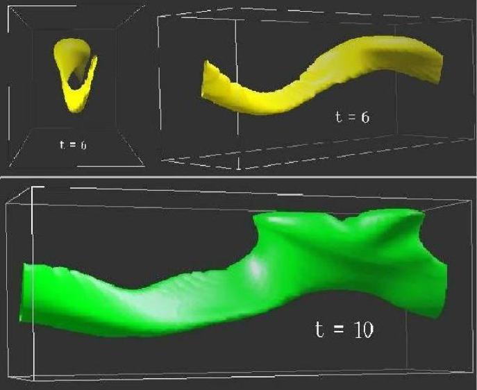
Fig. 4: Three-dimensional visualization of a rising flux tube in the presence of rotation. The stratification is adiabatic such that temperature, pressure, and density all vanish at a height that is about 30% above the vertical extent shown. (The actual computational domain was actually larger in the $x$ and $z$ directions.)

WHY SMALL SCALE LOSSES ARE GOOD

A relatively useful concept is based on the evolution equations for SS and LS fields under the assumption that the fields are maximally helical (or have known helicity fractions $\epsilon_{\rm m}$ and $\epsilon_{\rm f}$) and have opposite signs of magnetic helicity at small and large scales. The details can be found in Brandenburg, Dobler & Subramanian (2002, Sect. 4.2) and Blackman & Brandenburg (2003). The strength of this approach is that it is quite independent of mean-field theory.

Losses of large-scale field have been modeled using diffusion terms. The phenomenological evolution equation are written in terms of the LS and SS magnetic energies, $M_{\rm m}$ and $M_{\rm f}$ respectively, where we assume $M_{\rm m}=\pm\mu_{0}C_{\rm m}/k_{\rm m}$ and $M_{\rm f}=\mp\mu_{0}C_{\rm f}/k_{\rm f}$ for fully helical fields (upper/lower signs apply to northern/southern hemispheres). Here, $C_{\rm m}=\langle\overline{\mbox{\boldmath$J$}}\cdot\overline{\mbox{\boldmath$B$}}\rangle$ and $C_{\rm f}=\langle\mbox{\boldmath$j$}{}\cdot\mbox{\boldmath$b$}{}\rangle$ are the LS and SS current helicities. The phenomenological evolution equation for the LS energy then takes the form

$$k_{\rm m}^{-1}{{\rm d}M_{\rm m}\over{\rm d}t}=-2\eta_{\rm m}k_{\rm m}M_{\rm m}+2\eta_{\rm f}k_{\rm f}M_{\rm f},$$ (10)

where $\eta_{\rm m}$ and $\eta_{\rm f}$ are effective magnetic diffusivities that are expected to lie somewhere between between the molecular magnetic diffusivity, $\eta$, and the turbulent magnetic diffusivity, $\eta_{\rm t}$. The positive sign for the term involving $M_{\rm f}$ reflects the generation of the LS field from the SS. The case $\eta_{\rm m}=\eta_{\rm f}=\eta$ was already discussed by Brandenburg (2001) who assumed that the small scale magnetic field saturates at a certain time $t_{\rm sat}$, so that $M_{\rm f}\approx\mbox{const}$ for $t>t_{\rm sat}$. After that time, Eq. (10) can be solved to give

$$M_{\rm m}=M_{\rm f}\,{\eta_{\rm f}k_{\rm f}\over\eta_{\rm m}k_{\rm m}}\left[1-e^{-2\eta_{\rm m}k_{\rm m}^{2}(t-t_{\rm sat})}\right],\quad\mbox{for $t>t_{\rm sat}$}.$$ (11)

This equation shows three things:

• The time scale on which the large scale magnetic energy evolves depends only on $\eta_{\rm m}$, not on $\eta_{\rm f}$.

• The saturation amplitude diminishes as $\eta_{\rm m}$ is increased, which compensates the accelerated growth just past $t_{\rm sat}$ (Brandenburg & Dobler 2001).

• The reduction of the saturation amplitude due to $\eta_{\rm m}$ can be offset by having $\eta_{\rm m}\approx\eta_{\rm f}$, i.e. by having losses of small and large scale fields that are about equally important.

The overall conclusions that emerge are: (i) $\eta_{\rm m}>\eta$ is required if the large scale field is to evolve on a time scale other than the resistive one; (ii) $\eta_{\rm m}\approx\eta_{\rm f}$ is required if the saturation amplitude is not to be catastrophically diminished. These requirements are perfectly reasonable, but so far they have not been borne out by simulations. Brandenburg & Dobler (2001) found that most of the losses of magnetic helicity occur on large scale. This is at first glance very surprising, but on the other hand the magnetic helicity is a quantity that is strongly dominated by the large scales. However, certain phenomena such as CMEs and other perhaps less violent surface events are not presently included in the simulations. As vindication of the concept, however, it has been possible to show that the artificial removal of small scale magnetic fields (via Fourier filtering after a certain number of time steps) can indeed lead to significant increase of the saturation amplitude (Brandenburg, Dobler & Subramanian 2002). This is shown in Figure 5, where we show the evolution of the LS magnetic energy in a run where, in certain time intervals, magnetic energy is removed above the wavenumber $k=4$. Comparison with the original curve of Run 3 of Brandenburg (2001) shows that the removal of SS magnetic field allows the LS field to grow beyond the original limit, which is in agreement with the prediction from the phenomenology given by equation (11). Furthermore, and again in agreement with equation (11), the time scale for saturation is still the resistive time scale.

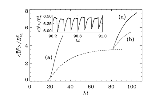
Fig. 5: The effect of removing small scale magnetic energy in regular time intervals $\Delta t$ on the evolution of the large scale field (solid lines). The dashed line gives the evolution of $\langle\overline{\mbox{\boldmath$B$}}^{2}\rangle$ for Run 3 of Brandenburg (2001), where no such energy removal was included. In all cases the field is shown in units of $B_{\rm eq}^{2}=\mu_{0}\rho_{0}\langle\mbox{\boldmath$u$}{}^{2}\rangle$. The two solid lines show the evolution of $\langle\overline{\mbox{\boldmath$B$}}^{2}\rangle$ after restarting the simulation from Run 3 of B01 at $\lambda t=20$ and $\lambda t=80$. Time is scaled with the kinematic growth rate $\lambda$. The curves labeled (a) give the result for $\Delta t=0.12\lambda^{-1}$ and those labeled (b) for $\Delta t=0.4\lambda^{-1}$. The inset shows, for a short time interval, the sudden drop and subsequent recovery of the total (small and large scale) magnetic energy in regular time intervals. [Adapted from Brandenburg, Dobler & Subramanian (2002).]

DISCUSSION

After having discussed the relation between LS and SS helical fields, and their significance to losses of helical fields through the solar surface, we can now restate the reasons why we expect there to be as yet undetected losses of large scale magnetic helicity of positive sign in the northern hemisphere and negative sign in the southern hemisphere. Because of magnetic helicity conservation, the observed magnetic helicity of one sign must be accompanied by magnetic helicity of the opposite sign (e.g. Blackman & Field 2000). Simulations have shown that contributions of opposite sign occur at different length scales, rather than at different positions in space. This leaves two possibilities: there could be a change of sign of magnetic helicity at a scale less than the resolution cutoff of about 80 km, or there could be magnetic helicity at a scale comparable to the size of the entire sun. There are two argument in favor of the latter possibility. (i) According to standard expectations, the $\alpha$-effect should be positive (negative) in the northern (southern) hemisphere. Since the $\alpha$-effect produces the field on the scale of the Sun, the helicity of the latter should also be positive (negative) in the northern (southern) hemisphere. (ii) If $\alpha$ had the opposite sign (as found for example in simulations of accretion disc dynamos; see Brandenburg et al. 1995), the observed losses would be associated with large scale field. Predominant large scale losses would however diminish the magnitude of the observed large scale field, to a level probably far below equipartition.

CONCLUDING REMARKS

The magnetic helicity equation has proved to be a valuable tool in understanding mean-field dynamos based on helicity effects. This tool is most successful in connection with homogeneous dynamos, where the kinetic helicity distribution is uniform. Of great interest is of course the nonuniform case that has been discussed in a number of recent papers by Kleeorin et al. (2000, 2002). The problems that arise if one relaxes the restrictions to nonuniformity can be traced back to the absence of gauge invariant formulations of the helicity equation in that sense (Brandenburg 2003). Because of these difficulties we have here adopted a more phenomenological approach where the helicity gradient terms are simply modeled as diffusion terms.

Simulations with open boundaries and stratification are needed to check whether more realistic dynamos always exhibit bi-helical behavior, as suggested in the present work. This is also related to the question of the observational appearance of bi-helical features. In Blackman & Brandenburg (2003) we have suggested that the N and S-shaped sigmoidal structures could be a direct manifestation of bi-helical structure. Viewed from the top, the flux tube in Fig. 2 would look like a N, in agreement with what is expected from Joy’s law for the norther hemisphere, and like a S for the southern hemisphere. It would be an important validation of a simulation of large scale dynamo action if such sigmoidal structures could be obtained self-consistently.

References

- [1]
- [2] Abbett W. P., Fisher G. H. & Fan Y., “The three-dimensional evolution of rising, twisted magnetic flux tubes in a gravitationally stratified model convection zone,” Astrophys. J. 540, 548-562, 2000.
- [3]
- [4] Arlt, R. & Brandenburg, A., “Search for non-helical disc dynamos in simulations,” Astron. Astrophys. 380, 359-372, 2001.
- [5]
- [6] Bao, S. D., Zhang, H. Q., Ai, G. X. & Zhang, M., “A survey of flares and current helicity in active regions,” Astron. Astrophys. Suppl. 139, 311-320, 1999.
- [7]
- [8] Berger, M. & Field, G. B., “The topological properties of magnetic helicity,” J. Fluid Mech. 147, 133-148, 1984.
- [9]
- [10] Blackman, E. G. & Brandenburg, A., “Dynamic nonlinearity in large scale dynamos with shear,” Astrophys. J. 579, 359-373, 2002.
- [11]
- [12] Blackman, E. G. & Brandenburg, A. “Doubly helical coronal ejections from dynamos and their role in sustaining the solar cycle,” Astrophys. J. Lett. (in press) 2003. (astro-ph/0212010)
- [13]
- [14] Blackman, E. G. & Field, G. B., “Coronal activity from dynamos in astrophysical rotators,” Monthly Notices Roy. Astron. Soc. 318, 724-732, 2000.
- [15]
- [16] Blackman, E. G. & Field, G. B., “New dynamical mean-field dynamo theory and closure approach,” Phys. Rev. Letters 89, 265007-, 2002.
- [17]
- [18] Brandenburg, A., “The inverse cascade and nonlinear alpha-effect in simulations of isotropic helical hydromagnetic turbulence,” Astrophys. J. 550, 824-840, 2001.
- [19]
- [20] Brandenburg, A., “The helicity issue in large scale dynamos,” In Simulations of magnetohydrodynamic turbulence in astrophysics (ed. T. Passot & E. Falgarone), Springer Lecture Notes in Physics, 2003 (to appear). (astro-ph/0207394)
- [21]
- [22] Brandenburg, A. & Dobler, W., “Large scale dynamos with helicity loss through boundaries,” Astron. Astrophys. 369, 329-338, 2001.
- [23]
- [24] Brandenburg, A., Dobler, W. & Subramanian, K., “Magnetic helicity in stellar dynamos: new numerical experiments,” Astron. Nachr. 323, 99-122, 2002. (astro-ph/0111567)
- [25]
- [26] Brandenburg, A., Nordlund Å., Stein, R. F. & Torkelsson, U., “Dynamo generated turbulence and large scale magnetic fields in a Keplerian shear flow,” Astrophys. J. 446, 741-754, 1995.
- [27]
- [28] Choudhuri, A. R., Schüssler, M. & Dikpati, M., “The solar dynamo with meridional circulation,” Astron. Astrophys. 303, L29-L32, 1995.
- [29]
- [30] Démoulin, P., Mandrini, C. H., van Driel-Gesztelyi, L., Lopez Fuentes, M. C., & Aulanier, G., “The magnetic helicity injected by shearing motions,” Solar Phys. 207, 87-110, 2002.
- [31]
- [32] Durney, B. R., “On a Babcock-Leighton dynamo model with a deep-seated generating layer for the toroidal magnetic field. II,” Solar Phys. 166, 231-260, 1995.
- [33]
- [34] Field, G. B. & Blackman, E. G., “Dynamical quenching of the dynamo,” Astrophys. J. 572, 685-692, 2002.
- [35]
- [36] Glatzmaier, G. A. & Roberts, P. H., “A three-dimensional self-consistent computer simulation of a geomagnetic field reversal,” Nature 377, 203-209, 1995.
- [37]
- [38] Kleeorin, N. I, Moss, D., Rogachevskii, I. & Sokoloff, D., “Helicity balance and steady-state strength of the dynamo generated galactic magnetic field,” Astron. Astrophys. 361, L5-L8, 2000.
- [39]
- [40] Kleeorin, N. I, Moss, D., Rogachevskii, I. & Sokoloff, D., “The role of magnetic helicity transport in nonlinear galactic dynamos,” Astron. Astrophys. 387, 453-462, 2002.
- [41]
- [42] Kulsrud, R. M. & Anderson, S. W., “The spectrum of random magnetic fields in the mean field dynamo theory of the galactic magnetic field,” Astrophys. J. 396, 606-630, 1992.
- [43]
- [44] Longcope, D. W. & Klapper, I., “Dynamics of a thin twisted flux tube,” Astrophys. J. 488, 443-453, 1997.
- [45]
- [46] Pevtsov, A. A., Canfield, R. C. & Metcalf, T. R., “Latitudinal variation of helicity of photospheric fields,” Astrophys. J. 440, L109-L112, 1995.
- [47]
- [48] Pouquet, A., Frisch, U. & Léorat, J., “Strong MHD helical turbulence and the nonlinear dynamo effect,” J. Fluid Mech. 77, 321-354, 1976.
- [49]
- [50] Seehafer, N., “Electric current helicity in the solar photosphere,” Solar Phys. 125, 219-232, 1990.
- [51]
- [52] Steenbeck, M., Krause, F. & Rädler, K.-H., “Berechnung der mittleren Lorentz-Feldstärke für ein elektrisch leitendendes Medium in turbulenter, durch Coriolis-Kräfte beeinflußter Bewegung,” Z. Naturforsch. 21a, 369-376, 1966. See also the translation in Roberts & Stix, The turbulent dynamo, Tech. Note 60, NCAR, Boulder, Colorado (1971).
- [53]
- [54] Stenflo, J. O., “Global wave patterns in the Sun’s magnetic field,” Astrophys. Spa. Sci. 144, 321-336, 1988.
- [55]
- [56] Stenflo, J. O., Güdel, M., “Evolution of solar magnetic fields: modal structure,” Astron. Astrophys. 191, 137-148, 1988.
- [57]
- [58] Stenflo, J. O., Vogel, M., “Global resonances in the evolution of solar magnetic fields,” Nature 319, 285-290, 1986.
- [59]
- [60] Stix, M., “Differential rotation and the solar dynamo,” Astron. Astrophys. 47, 243-254, 1976a.
- [61]
- [62] Stix, M., “Dynamo theory and the solar cycle,” In Basic Mechanisms of solar activity (ed. V. Bumba & J. Kleczek), pp. 367-388. IAU Symp. 71, 1976b.
- [63]
- [64] Vainshtein, S. I. & Cattaneo, F., “Nonlinear restrictions on dynamo action,” Astrophys. J. 393, 165-171, 1992.
- [65]
- [66] Vishniac, E. T. & Cho, J., “Magnetic helicity conservation and astrophysical dynamos,” Astrophys. J. 550, 752-760, 2001.
- [67]
- [68] Yoshimura, H., “Phase relation between the poloidal and toroidal solar-cycle general magnetic fields and location of the origin of the surface magnetic fields,” Solar Phys. 50, 3-23, 1976.
- [69]
- [70] Zheligovsky, V. A., Podvigina, O. M. & Frisch, U., “Dynamo effect in parity-invariant flow with large and moderate separation of scales,” Geophys. Astrophys. Fluid Dynam.95, 227-268, 2001.
- [71]