Magnetic helicity evolution in a periodic domain with imposed field
Axel Brandenburg
NORDITA, Blegdamsvej 17, DK-2100 Copenhagen Ø, Denmark
William H. Matthaeus
University of Delaware, Bartol Research Institute, 217 Sharp Lab, Newark, DE 19806
(, Revision: 1.58 )
Abstract
In helical hydromagnetic turbulence with an imposed magnetic field
(which is constant in space and time)
the magnetic helicity of the field within a periodic domain
is no longer an invariant of the ideal equations.
Alternatively, there is a generalized magnetic helicity that is an
invariant of the ideal equations.
It is shown that this quantity is
not gauge invariant and that it can therefore not be used in practice.
Instead, the evolution equation of the magnetic helicity of the
field describing the deviation from the imposed field is shown to
be a useful tool.
It is demonstrated that this tool can determine steady state quenching
of the alpha-effect.
A simple three-scale model is derived to describe the
evolution of the magnetic helicity and to predict its sign as
a function of the imposed field strength.
The results of the model agree favorably with simulations.
pacs:
52.65.Kj, 47.11.+j, 47.27.Ak, 47.65.+a
††preprint: NORDITA 2003-29 AP
I Introduction
Magnetic helicity has traditionally been used as a diagnostic
tool to characterize magnetic field topology. Only in
recent years magnetic helicity has also become a useful tool in
understanding large scale dynamo action.
Magnetic helicity is important because it is conserved
in the limit of vanishing resistivity.
This is not the case with the kinetic helicity, which is also
conserved in the inviscid case, but the kinetic helicity dissipation rate
diverges in the inviscid limit BK01 .
In this sense kinetic helicity is not even approximately conserved at
large Reynolds numbers, while magnetic helicity is very nearly conserved
at large magnetic Reynolds numbers Ber84 .
A key result that has emerged
from the concept of magnetic helicity conservation is that,
in a periodic domain, a large scale magnetic field generated by
the -effect Mo78 ; KR80 saturates on a resistive
time scale B01 . This time scale can be very long.
The helicity concept has also provided us with
a simple explanation for the final saturation field strength of
helical dynamos in periodic domains; see Ref. B01 for details.
In this light, the case with an imposed magnetic field has also been considered
MMMD02 ; MMD03 , where it was found that above a certain
field strength the dynamo is suppressed.
In the present paper we use similar ideas to obtain a more detailed
understanding of the case with an imposed field.
We begin with the equation governing the evolution of the
magnetic helicity in a periodic domain in the presence of an imposed
field. It is well known that in that case the magnetic helicity of
the fluctuating magnetic field is no longer conserved in the nonresistive
limit MG82 , but we also point out that a certain
generalized (or total) magnetic helicity that has sometimes been used
instead is gauge dependent and can therefore not be used in the present
case.
We then discuss applications of the magnetic helicity equation to
the alpha-effect in mean-field electrodynamics and derive a model
equation in order to understand the evolution of the magnetic helicity
for different imposed field strengths.
II Magnetic helicity equation
The evolution of the magnetic field is governed by
(1)
where the electric field is obtained from Ohm’s law,
(2)
where is the velocity, the current density,
and the resistivity.
Throughout this paper we adopt SI units,
but we set the permeability to unity.
We consider all quantities to be triply-periodic
over a cartesian domain.
We consider the case with a finite mean field,
(3)
where angular brackets denote full volume averages.
Such averages have no spatial dependence, but they can
still depend on time.
However, because of periodicity, the volume average of the
curl in Eq. (1) vanishes, and hence .
In other words, is not only constant in space,
but it is also constant in time.
Next, we split the field into a mean and a fluctuating component,
,
and introduce the magnetic vector potential for the
fluctuating component via ,
where is periodic.
The uncurled induction equation reads
(4)
where is the scalar potential.
We now consider the magnetic helicity.
The imposed field is constant in space and does therefore
not contribute to the magnetic helicity.
We therefore consider only the magnetic helicity
of the fluctuating field, .
This quantity is gauge invariant because adding a gradient
term to does not change :
(5)
Here we have used the solenoidality of , and the fact that the
volume average over a divergence term vanishes for a periodic domain.
The equation for the (gauge-dependent)
helicity density of the fluctuating
field can be obtained in the form
(6)
The divergence term vanishes after volume averaging, so
(7)
where all terms are gauge-independent.
Making use of Eq. (2), we have
(8)
where we have used .
Equation (8) can also be written as
(9)
where the electromotive force, ,
has been introduced.
If the flow is isotropic and helical, there will be an -effect
Mo78 ; KR80 ; B01 with , so
(10)
(In Appendix A we clarify the implications of
a finite effect when the Faraday displacement current is
restored in the Maxwell equations and when it is ignored.)
Since is gauge invariant, it is a physically
meaningful quantity. If there is a steady state, then
must also be steady. In that case we have
(11)
which is a relation due to Keinigs Kei83 for the -effect
in the saturated (steady) state;
see also Ref. MGL86 . If the field is weak, the
-effect will remain finite in the high conductivity
limit KR80 .
The presence of a finite -effect means that the structure
of Eq. (11) is very different when there is an imposed field.
Unlike the case without imposed field (), the quantity
is no longer conserved in the limit .
This prompted Matthaeus & Goldstein MG82 to consider the
quantity
(12)
where
(13)
Note that is constructed such that it satisfies the equation
(14)
Indeed, this equation reduces to Eq. (9) after inserting
Eqs (12) and (13) into (14).
The symbol is chosen to make the extra term in
Eq. (12) look like a magnetic helicity, even though
.
The reason for is that
corresponds to a slowly varying variable, whose curl gives at
a higher order, and not the order we are working in; see Eq. (A9)
of Ref. Stribling_etal1994 .
Conversely, corresponds to the curl of at a lower order.
A rigorous scale expansion is given in the Appendix of
Ref. Stribling_etal1994 .
In the nonresistive limit, the right hand side of Eq. (14)
vanishes, and so is conserved. One may be tempted to
conclude that in the steady state, . This is not
generally true, however, and it would be in conflict with
Eqs (10) and (11). Certainly for sufficiently
weak fields is finite VC92 ,
so will also remain
finite, see Eq. (11). Therefore, cannot be constant in
the steady state. The reason for this puzzle
is that is not gauge invariant Ber97 , because
the definition of involves the quantity . At first
glance, appears to be gauge invariant,
because is gauge invariant
and involves only a time
integral over ; see Eq. (13). However, the beginning of the time
integration is ill-defined, so in general one can replace
(15)
which would lead to a different conserved
magnetic helicity, , where
is undetermined.
Therefore, is not a physically meaningful quantity,
so it is not surprising that can have a
component that grows linearly in time.
We emphasize however that is still gauge
invariant and therefore physically meaningful, even though it is no
longer a conserved quantity in the ideal limit.
III Non-periodic gauge potentials
In this section we want to comment on the related issue that adding a
spatially constant vector to the right hand side of Eq. (4)
would not affect the evolution of .
The constant vector can readily be absorbed in the definition
of the scalar potential , because it is specified only up to an
additional gauge potential.
However, this gauge potential has in general a
non-periodic contribution, even when all other quantities are periodic.
More specifically, in Eq. (4)
must have an additional component that varies
linearly in space, i.e.
(16)
where is periodic and is the position vector.
We stress that in Eq. (16) is therefore in general not periodic,
even if and are periodic.
A comment on the helicity flux associated with the gauge field is here
in order.
This flux is often written as which would then not be periodic
and hence it is not obvious that its surface integral vanishes; see
Eqs (6) and (7).
(The importance of this term for magnetic helicity injection has been
discussed in Ref. JC84 .)
However, using the identity
(17)
the magnetic helicity flux can also be written as
, which is periodic.
Therefore, there is no contribution from the term in our case.
(We note that similar manipulations can be used to turn a
non-periodic vector potential into a periodic one if the velocity
is a linear function of coordinates BNST95 .)
The term has recently been discussed in a
formulation of a magnetic helicity conserving dynamo effect VC01 .
Obviously, such a term does not give a contribution under the
divergence and hence cannot be physically meaningful AB01 .
IV Application to -quenching
There have been a number of simulations of helically forced periodic
flows with an imposed magnetic field.
The general objective is to obtain the -effect and its suppression
as a function of field strength B01 ; TCV93 ; CH96 .
In the steady state, Eq. (11) can be used to determine
by measuring in a simulation with an applied
magnetic field .
For helical turbulence, can be approximated by
(18)
where
for a fully helical field with positive or negative helicity, and
for fractional helicity.
A strongly helical small scale magnetic field is generally expected when
the turbulent velocity field is also strongly helical PFL76 .
The steady state is therefore given by
(19)
On the other hand, the kinematic value of
can be estimated in terms of the kinetic helicity,
(20)
where is the correlation time which, in turn, can be expressed
in terms of the turbulent magnetic diffusivity for which we have a
similar expression, .
In analogy to Eq. (18), we write
, so
(21)
If we assume that the small scale field is in equipartition, i.e. ,
and if we define BB02 the magnetic Reynolds number as
, then Eq. (21)
can be turned into the interpolation formula,
(22)
that recovers Eq. (21) for strong fields and
in the weak field limit, .
This equation is known as the catastrophic quenching formula of
Vainshtein and Cattaneo VC92 .
In order to confirm that the onset of steady state quenching depends on the
magnetic Reynolds number based on the forcing scale FB02 ,
, and not on the
magnetic Reynolds number based on the scale of the box B01 ,
,
we show two series of simulations obtained for different values of
the forcing wavenumber , for different values of .
The forcing of the flow was fully helical; for details on the
numerical method see Ref. B01 .
The result is shown in Fig. 1.
Figure 1:
Normalized -effect versus normalized magnetic energy, scaled
with the small scale magnetic Reynolds number (upper panel)
and the large scale magnetic Reynolds number (lower panel).
Note that the onset of quenching is governed by the small scale magnetic
Reynolds number, not the large scale magnetic Reynolds number.
Next, we consider simulations where we use hyperdiffusivity, i.e. the
ordinary magnetic diffusion operator, , is replaced
by , where corresponds to the standard case.
This is a common tool in order to extend the inertial range of the
turbulence MFP81 , but it is also clear that this leads to wrong
saturation field strengths BS02 .
In the presence of hyperdiffusivity, the magnetic Reynolds number is
defined as .
In the following we show, however, that the quenching data are better
described by a single quenching curve when is rescaled,
(23)
The result is shown in Fig. 2.
The factor of 1.6 is not expected to be universal but is probably
a slowly varying function of magnetic Reynolds number BS02 ; BB02 .
Figure 2:
Normalized -effect versus magnetic field strength.
The full dots denote runs where hyperdiffusion has been used. In the second
panel, is scaled with the magnetic Reynolds number
based on the forcing scale, . The last panel is similar to the
second, but the effective forcing wavenumber has been used which is
scaled by a factor 1.6. This brings especially the hyperdiffusive
runs (full dots) closer to the rest of the data points.
We conclude that Eq. (22) describes the simulations quite well
provided the magnetic Reynolds number is defined in a suitable manner.
We emphasize however that this equation only applies to the
steady state and if there is no mean current.
This is generally not the case
and therefore the quenching is in practice not automatically
catastrophic BB02 , i.e. the onset of quenching does not depend on .
V Evolution of large scale magnetic helicity
Recently, the effect of an imposed
field on the inverse cascade has been studied MMMD02 ; MMD03 . If
the imposed magnetic field is weak or absent, there is a strong nonlocal
transfer of magnetic helicity and magnetic energy from the forcing scale
to larger scales. This leads eventually to the accumulation of magnetic
energy at the scale of the box B01 ; MFP81 ; BP99 . As the strength
of the imposed field (wavenumber ) is increased, the accumulation
of magnetic energy at the scale of the box () becomes more
and more suppressed MMMD02 .
Qualitatively, this can be understood as the result of two competing
effects: (i) the inverse cascade that produces magnetic helicity of
opposite sign at compared to that at the forcing wavenumber ,
and (ii) the -effect operating on the imposed field producing
magnetic helicity of the same sign at than at .
This is because the sign of the -effect is opposite to the sign of
the magnetic helicity at , and enters with a minus
sign in the evolution equation (10) of magnetic helicity.
Under the assumption that the turbulence is fully helical,
the critical value of the imposed field can be estimated by
balancing the two terms on the right hand side of
Eq. (10) and by approximating, as in § IV,
and .
This yields
(24)
where the last equality is again to be understood as
a definition of the magnetic Reynolds number, see also Ref. BB02 .
For the sign of the magnetic helicity is the same both at
and at , while for the signs are opposite.
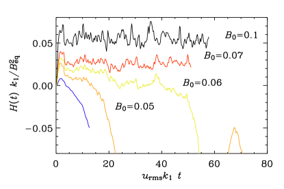
Figure 3:
Evolution of the total magnetic helicity, ,
as a function of for different
values of , as obtained from the three-dimensional simulation.
A related phenomenological model for saturation of the dynamo effect
under influence of has been given MMD03
that is based upon a Fourier scale separation approach. That approach
leads the conclusion that the critical value rather
than as above. Further analysis may be needed to fully
reconcile the differences in these approaches, both of which appear to have
some support from simulations.
A more quantitative description of the evolution of the magnetic helicity
can be obtained by using a modified two-scale model FB02 ; BB02 ,
where the term from Eq. (9) has been
included, so
(25)
(26)
Here, and are the magnetic helicities at the wavenumbers
and , respectively, and is
the helicity production from -effect and turbulent diffusion
operating on the field at .
We note that the sum of Eqs (25) and (26) yields Eq. (7).
The electromotive force at wavenumber is given by
(27)
To calculate in Eqs (25) and (26) we dot
Eq. (27) with , volume average, and note that
and .
The latter relation assumes that the field at wavenumber is fully
helical, but that it can have either sign.
Thus, we have
(28)
The large scale magnetic
helicity production from the -effect operating on the
imposed field is .
The -effect is proportional to the residual magnetic helicity
of Pouquet, Frisch and Léorat PFL76 , with
(29)
where is the correlation time and the average density.
In terms of and we write
(30)
(31)
for the -effect with feedback from and ,
respectively.
Here, is the contribution to the -effect
from the kinematic helicity, as defined in Eq. (20).
The above set of equations for the case of an imposed magnetic field
is similar to a recently proposed four-scale model Bla03 , where two
smaller scales were added relative to the two-scale model.
In the present case, on the other hand, instead of including scales
smaller than the forcing scale, the imposed field at the infinite scale
is included, albeit fixed in time.
For finite values of , the final value of is particularly
sensitive to the value of and turns out to be too
large compared with the simulations.
This disagreement with simulations
is readily removed by taking into account that
should itself be quenched
when becomes comparable to .
Thus, we write
(32)
which is a good approximation to more elaborate expressions RK93 .
We emphasize that this equation only applies to and is
therefore distinct from Eq. (22).
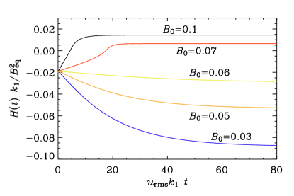
Figure 4:
Evolution of magnetic helicity as a function of for different
values of , as obtained from the two-scale model.
In Fig. 4 we show the result of a numerical integration of
Eqs (25) and (26).
Both the three-dimensional simulation and the two-scale model show a
similar value of , above which changes sign.
This confirms the validity of our estimate of the critical value
obtained from Eq. (24).
Secondly, the time evolution is slow when and faster when
.
In the simulation, however, the field attains its final level
for almost instantaneously, which is not the case in the model.
It is possible MMD03 that the almost instantaneous adjustment in
the simulations is a consequence of the Alfvén effect, which is not
included in the present model.
This, and other shortcomings of the present model may also be responsible
for the mismatch between the magnetic helicity amplitudes seen in the
simulations and the model.
Most characteristic in the simulations is the fact that while
in the limit of strong imposed field strength.
VI Conclusions
We have shown that (i) in the presence of an imposed field and (ii)
using triple-periodic boundary conditions, the generalized magnetic
helicity MG82 in Eq. (12) is not gauge-invariant and can
therefore not be used for practical purposes.
This quantity has frequently been used in the solar wind community
as an alternative to the ordinary magnetic helicity which is known
not to be conserved in the limit of vanishing resistivity.
We have argued, however, that even through the ordinary magnetic helicity is
not conserved in the presence of an imposed field and in the limit of
low resistivity, it remains an extremely useful quantity that has
predictive power – similar to the case without imposed field B01 .
Based on analytic considerations and confirmed by the simulations,
we have shown that the sign of the magnetic helicity depends on
the strength of the imposed magnetic field.
If the field is weak enough, the situation is similar to the case
without imposed magnetic field and the sign of the magnetic helicity
is opposite to the sign of the helicity of the turbulence.
If the field exceeds a certain threshold, which is
times the equipartition field strength, where is the magnetic
Reynolds number based on the forcing wavenumber, the sign of magnetic
helicity changes and becomes equal to the sign of the helicity of the
turbulence.
This can be understood as a consequence of the -effect
operating on the imposed field.
In finite systems, this -effect would cause the large scale
field to have opposite helicity compared to the small scale field.
In an infinite (or periodic) system, this is not possible, and the
entire field in the computational domain plays the role of a small scale field which
must then have the same sign of helicity as the turbulence.
The two-scale model used to describe the nonlinear evolution of helical
dynamos FB02 ; BB02 can be generalized to take account of the
large scale field.
The formalism is similar to a recently proposed four-scale model
Bla03 .
The nonlinear two-scale and multi-scale models play important roles
in modern mean-field dynamo theory.
Given that we are still lacking a proper understanding of solar and
stellar dynamos in the nonlinear regime, an independent confirmation
of the nonlinear multi-scale model must therefore be regarded as a
crucial step toward understanding the origin and maintenance of
magnetic fields in turbulent astrophysical bodies.
Acknowledgements.
We thank the referee for inspiring us to comment on the role
of the displacement current in triply periodic systems,
Eric Blackman for comments on the manuscript,
and George Field for organizing the workshop at Virgin Gorda,
where we started working on this paper.
The Danish Center for Scientific Computing is acknowledged for
granting supercomputing time on the Horseshoe machine in Odense.
Appendix A The role of the displacement current in triply periodic systems
with imposed field
In this appendix we discuss a paradoxical situation MB99 that
arises when comparing volume averages of the present equations (where
periodic boundary conditions are used and a uniform field is imposed) with
the full Maxwell equations (where the displacement current is included).
The displacement current is given by the fourth Maxwell equation,
(33)
where is the speed of light.
We recall that the permeability has been put to unity.
Applying volume averages, and noting that the volume average of the
curl vanishes, we have
(34)
On the other hand, the volume average of Ohm’s law (2) yields
(35)
We assume that there is no net flow, i.e. .
Therefore, .
In helical hydromagnetic turbulence there is an
-effect Mo78 ; KR80 ; B01 , so
,
and therefore and, because of
Eq. (34), .
The latter condition is, of course, inconsistent with our
assumption that .
This discrepancy could be particularly important when considering
the contribution of the volume averaged field to the Lorentz force,
, which vanishes in the pre-Maxwellian MHD
approximation, but not when the displacement current is retained
MB99 .
where the dot on denotes time differentiation.
Equation (36) could be solved for either in terms of the Green’s
function or via series expansion MB99 ,
confirming that .
However, here we are interested in the Lorentz force, so we write
(37)
The right hand side of Eq. (37) vanishes, because
is independent of time and
is parallel to .
The use of the equation ignores random fluctuations
in time about zero.
In that sense, Eq. (37) is strictly valid only when the averages
are also taken over time.
Table 1:
Comparison of various volume averages in the pre-Maxwellian approximation
and the full Maxwell equations.
The asterisk denotes that this result is strictly valid only when also
a time average is considered.
pre-Maxwell
Maxwell
The solution to Eq. (37) shows that,
if the Lorentz force from the mean field was vanishing initially,
it must vanish at all times.
Table 1 summarizes which of the different volume averages discussed
in this section vanish in the pre-Maxwellian MHD approximation and which
quantities remain finite when the full Maxwell equations are used.
The apparent inconsistency is removed by noting that Eq. (33)
does simply not exist in the pre-Maxwellian MHD formulation
and hence cannot be invoked in the discussion.
[The situation is similar to the incompressibility assumption,
,
or the anelastic approximation, , both of
which do not imply .
Indeed, the original continuity equation is no longer used and
has instead been replaced by
or , respectively.]
Nevertheless, as far as the Lorentz force is concerned, the
neglect of the displacement current is inconsequential,
because it vanishes in either of the two cases; see Table 1.
The mismatch between in the pre-Maxwellian
approximation and the exact result, , is negligible,
but can be quantified using a rigorous expansion in terms of slowly and
rapidly varying variables Stribling_etal1994 .
Such an approach also demonstrates quite nicely that the difficulties
introduced into the periodic model by the presence of a nonzero uniform
mean field are due to imposing periodic boundary conditions on the entire
(infinite volume) system.
If instead (see Appendix of Ref. Stribling_etal1994 ) the turbulence
is assumed to be modeled as locally homogeneous, in the statistical
sense, and periodicity is employed in a two scale expansion as a local
leading order model, no such problems emerge.
Paradoxical situations arising from the assumption of triple periodicity
are commonly resolved using scale expansion.
Another such example is the famous Jeans swindle BT87 , where the
assumed zero order equilibrium state does not obey triple periodicity;
see Refs Spitzer78 ; Chavanis02 for a stability analysis using a
proper equilibrium solution.
We emphasize, however, that the problem with the Jeans swindle is
distinct from the problem with the displacement current discussed here.
The latter is completely resolved by staying fully within the pre-Maxwellian
formulation, while the former is a true mathematical swindle.
References
(1)
Brandenburg, A., & Kerr, R. M., (ed. Quantized Vortex Dynamics and Superfluid Turbulence), pp. 358. C.F. Barenghi, R.J. Donnelly, W.F. Vinen (2001).
Lecture Notes in Physics, Vol. 571, Springer Verlag
(2)
M. Berger, Geophys. Astrophys. Fluid Dynam. 30, 79 (1984).
(3)
H. K. Moffatt Magnetic Field Generation in Electrically Conducting Fluids. Cambridge University Press, Cambridge (1978).
(4)
F. Krause and K.-H. Rädler Mean-Field Magnetohydrodynamics and Dynamo Theory. Akademie-Verlag, Berlin; also Pergamon Press, Oxford (1980).
(5)
A. Brandenburg, Astrophys. J. 550, 824 (2001).
(6)
D. Montgomery, W. H. Matthaeus, L. J. Milano, and
P. Dmitruk, Phys. Plasmas 9, 1221 (2002).
(7)
L. J. Milano, W. H. Matthaeus, and P. Dmitruk, Phys. Plasmas 10, 2287 (2003).
(8)
W. H. Matthaeus and M. L. Goldstein, J. Geophys. Res. 87, 6011 (1982).
(9)
R. K. Keinigs, Phys. Fluids 26, 2558 (1983).
(10)
W. H. Matthaeus, M. L. Goldstein, and S. R. Lantz, Phys. Fluids 29, 1504 (1986).
(11)
T. Stribling, W. H. Matthaeus, and S. Ghosh, J. Geophys. Res. 99, 2567 (1994).
(12)
S. I. Vainshtein and F. Cattaneo, Astrophys. J. 393, 165 (1992).
(13)
M. A. Berger, J. Geophys. Res. A 102, 2637 (1997).
(14)
T. H. Jensen and M. S. Chu, Phys. Fluids 27, 2881 (1984).
(15)
A. Brandenburg, Å. Nordlund, R. F. Stein, and
U. Torkelsson, Astrophys. J. 446, 741 (1995).
(16)
E. T. Vishniac and J. Cho, Astrophys. J. 550, 752 (2001).
(17)
R. Arlt and A. Brandenburg, Astron. Astrophys. 380, 359 (2001).
(18)
L. Tao, C. Cattaneo, S. I. Vainshtein, (ed. Solar and Planetary Dynamos), pp. 303. M. R. E. Proctor, P. C. Matthews & A. M. Rucklidge (1993).
Cambridge University Press
(19)
F. Cattaneo and D. W. Hughes, Phys. Rev. E 54, R4532 (1996).
(20)
A. Pouquet, U. Frisch and J. Léorat, J. Fluid Mech. 77, 321 (1976).
(21)
E. G. Blackman and A. Brandenburg, Astrophys. J. 579, 359 (2002).
(22)
G. B. Field and E. G. Blackman, Astrophys. J. 572, 685 (2002).
(23)
M. Meneguzzi, U. Frisch, U., Pouquet, A., Phys. Rev. Lett. 47, 1060 (1981).
(24)
A. Brandenburg and G. S. Sarson, Phys. Rev. Lett. 88, 055003 (2002).
(25)
D. Balsara and A. Pouquet, Phys. Plasmas 6, 89 (1999).
(26)
E. G. Blackman, Monthly Notices Roy. Astron. Soc. 344, 707 (2003).
(27)
G. Rüdiger and L. L. Kitchatinov, Astron. Astrophys. 269, 581 (1993).
(28)
D. C. Montgomery and J. W. Bates, Phys. Plasmas 6, 2727 (1999).
(29)
J. Binney and S. Tremaine Galactic dynamics. Princeton University Press, Princeton, New Jersey, pp. 287 (1987).
(30)
L. Spitzer, Jr. Physical processes in the interstellar medium. J. Wiley & Sons, New York, §13.3 (1978).
(31)
P. H. Chavanis, Astron. Astrophys. 381, 340 (2002).