Secondary proton flux induced by cosmic ray interactions with the atmosphere

Abstract

The atmospheric secondary proton flux is studied for altitudes extending from sea level up to the top of atmosphere by means of a 3-dimensional Monte-Carlo simulation procedure successfully used previously to account for flux measurements of protons, light nuclei, and electrons-positrons below the geomagnetic cutoff (satellite data), and of muons and antiprotons (balloon data). The calculated flux are compared with the experimental measurements from sea level uo to high float ballon altitudes. The agreement between data and simulation results are very good at all altitudes, including the lowest ones, where the calculations become extremely sensitive to the proton production cross section. The results are discussed in this context. The calculations are extended to the study of quasi trapped particles above the atmosphere to about 5 Earth radii, for prospective purpose.

I Introduction

The study of the particle flux in the earth neighbourhood has regained some interest recently with the emergence of a new generation of embarked experiments both at balloon and satellite altitudes. In this context, new measurements of the proton flux have been performed FR99 ; FU01 , providing a broad set of accurate data which could be compared to the latest generation of calculations. This is a quite compelling test which concerns the atmospheric flux of all secondary particles as well, since the latter are driven by $p$ induced cross sections along the atmospheric cascade. The interaction dynamics of the incident Cosmic Ray (CR) flux with the earth atmosphere and the earth magnetic field, for secondary particle production, is a complex process. So far it has been investigated only by means of a theoretical approach based on a diffusion equation PA96 . A new detailed study of this process through the body of recently measured data should significantly improve the current status of the knowledge in this matter, and it should validate the calculations based on this, or similar, simulation procedure for the evaluation of all the atmospheric secondary particle flux. It is also likely to improve our knowledge on the dynamics of the population of the radiation belts as well.

Studying the secondary proton flux in the atmosphere in this context is therefore of particular interest since it is highly sensitive to all the components of the simulation process, in particular to the secondary proton production cross section as discussed below. A successful account of this flux through the range of atmospheric altitudes is then likely to cast robust grounds to this approach in general, and to further validate the computation techniques used. Studying this flux at higher altitudes in the Earth environment on the basis establised previously should also be a useful investigation both from the point of view of the particle dynamics and for the future satellite experiments for which this background must be known.

The present work is a further step of a research program whose previous results on the flux of secondary atmospheric particles at satellite altitude, in particular on the interpretation of the AMS 98 measurements of protons, leptons, and light ions, below the geomagnetic cutoff (GC) PAP1 ; PAP2 ; PAP3 , and in the atmosphere (muons and neutrinos) LI03 , have been reported recently. The investigation of the proton flux reported in PAP1 is extended here to the atmospheric altitudes and to the high altitude region. The article reports on the calculated atmospheric $p$ flux from sea level to balloon altitude, on the comparison to the experimental data, and on the predictions of the flux at high altitudes from top of atmosphere (TOA) up to 3 10⁴ km. The main features of the calculations are described in section II. The production cross sections used in the event generator are briefly discussed in section III. The simulation results are discussed in section IV, while the transport equation approach is described and the results are shown in section V. The proton flux at high altitudes is reported in VI. The work is concluded in section VII.

The paper parallels a similar study on the antiproton flux in the earth environment HU03 , referred to as I in the following. The two papers are presented in this order for historical reasons.

II Simulation conditions

The flux of secondary atmospheric protons has been investigated using the same simulation approach used in PAP1 ; PAP2 ; PAP3 ; LI03 and for the antiproton (see I) flux in the atmosphere. The same computer code has been used here for the charged particle propagation in the terrestrial environment including the atmosphere, as in the previous studies. Incident CR proton and helium particles were generated and propagated inside the earth magnetic field, interacting with atmospheric nuclei according to their total reaction cross section and producing secondary nucleons $p$, $n$, light nuclei, leptons ($\mu,e^{\pm},\nu$) from meson ($\pi,K$) decay, and antinucleons $\overline{p}\;$, $\overline{n}\;$, with cross sections and multiplicities as discussed below. Each secondary particle produced in a given collision is propagated in the same conditions as incident CRs in the previous step, resulting in a more or less extended reaction cascade developing through the atmosphere, which included up to about ten generations of secondaries for the protons of the simulation sample PAP1 .

The reaction products are counted each time they are crossing, upwards or downwards, the virtual detection spheres. The locations of the latter were chosen between sea level and about 36 km for ground and balloon experiments (BESS, CAPRICE), at 380 km for the AMS satellite experiment, and beyond up to about 3 10⁴ km for the rest of the study. All charged particles undergo energy loss by ionisation in the atmospheric medium. Each event is propagated until the particle disappears by nuclear collision, stopping in the atmosphere by energy loss, or escaping to the outer space beyond twice the generation altitude (see PAP1 ; PAP2 ; PAP3 and I).

The incident CR proton and helium flux have been measured recently by several experiments BO99 ; ME00 ; SA00 ; PROT ; HELI . In the present work, functional form fits to the AMS data PROT ; HELI have been used in the calculations to generate the corresponding flux. For other periods of the solar cycle than those of the measurements, the incident cosmic flux were corrected for the different solar modulation effects using a simple force law approximation. The $A>4$ components of the CR flux were not taken into account in the present calculations (see ref LI03 for details).

III Cross sections

The inclusive $p+A\rightarrow p+X$ and ${}^{4}He+A\rightarrow p+X$ proton production cross sections and the proton and ⁴He total reaction cross sections on nuclei used here are described in I. For incident protons however, the description of the production cross section below 7.5 GeV BA85 used in PAP1 , has been constrained by the 4.2 GeV measurements from ref AG93 . This decreased the cross section over this range of energy by a few tens of percents. The details will be reported later.

The neutron production cross sections were taken the same as for protons. This is expected to be a good approximation for the incident and final state energies considered here. Charge-exchange reaction channels have been neglected in account of their small cross sections. The nucleon production from $He$ fragmentation were not included.

IV Results

Figure 1: Simulated proton flux in the atmosphere (histograms) compared to experimental results (symbols) between TOA and sea level. From top to bottom: CAPRICE TOA BO99 (full squares), CAPRICE 94 FR99 (7 altitudes: 29.9, 22.1, 17.5, 16, 12.6, 9.9, 5.75, in km), Kocharian et al., KO56 (3.2 km, full triangles), BESS FU01 (2.77km, full squares), Diggory et al., DI74 (sea level, inverted full triangles). See also BR64 for other data at sea level.

Figure 2: Rank distributions of the detected protons obtained from the simulation, for a set of altitudes between sea level and balloon high float altitude, showing the evolution of the mean production rank in the collision sequence, of the detected protons.

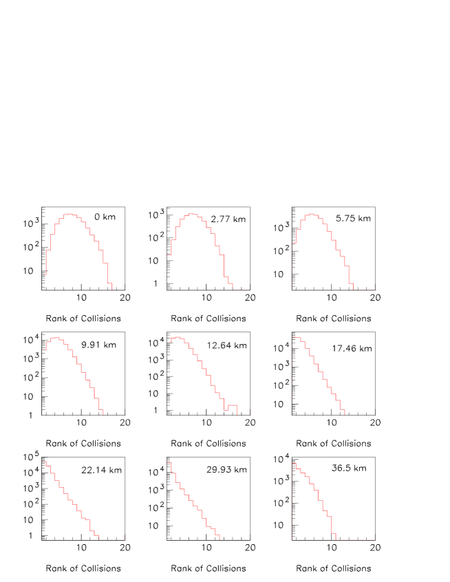
The proton flux in the atmosphere have been measured recently by the CAPRICE experiment between 5 and 29.9 km FR99 and at TOA BO99 , and by BESS at lower altitude (2.77 km) FU01 , while previous measurements were available from KO56 at 3.2 km, and from DI74 at sea level. This collection of data points is compared on figure 1 with the simulation results between sea level up to balloon altitudes. The comparison is remarkably good through the whole range of altitudes. Note that the calculations become increasingly sensitive to the proton production cross-section when going from high to low altitudes since all secondary protons result on the average from a sequence of $n$ collisions $N+A\rightarrow p+X$, $N$ standing for nucleon and $n$ being the average collision rank, involving (approximately) the same inclusive nucleon production cross section for each collision. Let the latter be noted as $\frac{d\sigma_{N}(E_{i},\theta,E)}{d\theta dE}$ for a given collision with $E_{i}$, $E$, $\theta$, being the nucleon incident energy, proton final energy, and production angle, respectively. Although the collisions involve different values of the kinematic variables, the final proton flux for a given altitude depends qualitatively on some appropriate average of the cross section above to the $n$th power, i.e.,: $<\!\frac{d\sigma_{N}(E_{i},\theta,E)}{d\theta dE}\!>^{n}$, with $n$ increasing with the decreasing altitude. Therefore the lower the altitude, the more sensitive the flux is expected to be to the inclusive proton production cross section.

Fig 2 shows a sample of rank distributions from sea level to ballon altitude obtaines from the simulation sample. The mean rank $n$ appears to drop from around 7 at sea level down to about 1.5 at 36.5 km. The flux is thus sensitive to approximately the 7th power of the cross section at sea level, while it depends only to the 3/2 power of this cross section, approximately, at ballon altitude. A discrepancy of a factor of 2 between calculation results and data at sea level can thus be considered as a good result since it would point to a discrepancy on the cross section of less than 10 percent.

These calculations thus provide an extremely sensitive test of the correctness of the cross sections used, and beyond of the overall method, and they assign a high confidence level to the all secondary particle flux calculated by this approach.

V The transport equation approach

The proton flux has also been calculated using the same diffusion equation approach as used in refs PF96 (see also PA96 ; ST97 ; ST93 ) in order to compare the two methods.

V.1 Numerical integration method

The equation to be solved can be written as:

$$\frac{\partial N_{i}}{\partial x}+\frac{\partial}{\partial E_{i}}\bigg{\langle}\frac{\partial E_{i}}{\partial x}\bigg{\rangle}N_{i}(x,E_{i})+\frac{N_{i}(x,E_{i})}{\lambda_{int}(E_{i})}$$ (1)

$${}-\sum_{A}\frac{1}{\langle m_{air}\rangle}\int_{E_{th}}^{\infty}\frac{d\sigma}{dE_{i}}(E_{i},E_{A})N_{A}(x,E_{A})dE_{A}=0$$

Where $i$ represents the transported particle species, $N_{i}(x,E_{i})$ its energy ($E_{i}$) dependent flux after crossing the thickness between $x$ and $x+dx$ (in $g/cm^{2}$)of (atmospheric) matter. The second term is the particle energy changing term accounting for energy loss by ionization (using the Bethe-Bloch formula). In the third (absorption) term, $\lambda_{int}$ is the particle interaction length derived from the total reaction cross section of the considered system. The last term is the source term, accounting for particle creation, with $A$ standing for the projectile-target system leading to the production of particle $i$. $\frac{d\sigma}{dE_{i}}(E_{i},E_{A})$ is the production cross section for particle $i$ in the system $A$ with incident energy $E_{A}$. The sum runs over all the allowed $A$ channels. The differential cross sections used here are the same (angle integrated) as used in the simulation. $\langle m_{air}\rangle$ is the mean nuclear mass of the atmospheric nuclei (14.58 amu).

The equation has been solved for the secondary proton flux at various altitudes. The technique used proceeds by the method of finite differences with implicit scheme proposed in ref. RECIP . It consists of solving a system of linear equations:

$$N_{n-1}^{m} = \frac{\Delta x}{\Delta E^{m-1}+\Delta E^{m}}\bigg{\langle}\frac{\partial E_{i}}{\partial x}\bigg{\rangle}^{m}(N_{n}^{m+1}-N_{n}^{m-1})+$$ (2)

$$(1+\frac{\Delta x}{\lambda^{m}})N_{n}^{m}-\frac{\Delta x}{\langle m_{air}\rangle}\sum_{m^{\prime}=1}^{M_{MAX}}\bigg{(}\frac{d\sigma^{m}}{dE}(E_{bin}^{m^{\prime}})+$$

$$\frac{d\sigma^{m}}{dE}(E_{bin}^{m^{\prime}+1})\bigg{)}\frac{\Delta E^{m^{\prime}}}{2}N_{n}^{m^{\prime}}$$

Where $m$ and $n$ are the index of the steps in energy and thickness crossed respectively.

For practical reasons related to the energy range to be covered versus the number of steps required and the size of the matrix to be inverted, the definition of the derivative used at the boundaries had to be modified to obtain stable calculation results RECIP .

V.2 Results

Figure 3: Results obtained using the diffusion equation approach for the transport of the proton flux in the atmosphere. The data are the same as in Fig. 1

Fig. 3 shows the results obtained in these calculations, compared to the same experimental data as in Fig. 1, at various altitudes in the atmosphere. The agreement is seen to be fair in the high altitude range, down to around 10 km. For the 5.5 km data, the observed disagreement is similar to that obtained by simulation, the data points having a much different energy behaviour than observed for the higher and lower energy spectra.

For altitudes lower than 5 km, significant disagreements between data and calculations appear, the latter overestimating the data by a factor of about 2 to 4. This disagrement probably originates in the one-dimension approximation of this approach. The difference between the 3-dimensional (3-D) approach of the simulation and the 1-dimension diffusion equation lies in a few 3-D effects not included in the latter approximation : a) The curvature of the particle in the magnetic field. b) The angle dependence of the particle production, 1-D approximation using the angle integrated cross section. A consequence of the above is that the effective path of particles in the atmosphere is longer than assumed in the 1-D approximation. Using the more realistic values of the path obtained in the simulation, in the diffusion equation brings only minor improvements to the observed disagreement. Introducing some cuts in the angular range of integration of the cross section distorts the resulting spectrum and does not improve the discrepancy either.

It is interesting to note that the failure of the 1-D approximation reported above at low atmospheric altitudes seems not to have a significant effect on the goodness of this approximation for the calculation of the atmospheric neutrino flux. This conclusion was reached on the basis of the fair agreement obtained between the 3-D and 1-D calculations in Ref.LI03 . This can be understood by the fact that the low altitude neutrino production represents less than 10% of the whole atmospheric production (fraction decreasing with the decreasing neutrino energy).

Figure 4: Simulation results for the altitude dependence of the downgoing (left) and upgoing (right) proton flux. Each set of curves of the two panels corresponds to a bin of geomagnetic latitude $\theta_{m}$ as indicated on the figure. The points and curves show the energy integrated primary flux of protons (full triangles), and the flux for proton with kinetic energies above 0.1 GeV (solid line), 0.3 GeV (dashed line), 1 GeV (solid line), and 3 GeV (dash-dotted line), respectively. See text for the discussion.

VI Secondary proton flux versus altitude

Figure 5: Same as figure 4 for the energy integrated downward proton flux (full triangle) and the E$>$0.1 GeV (full circles and solid line). The full circles symbols and dashed line show the fraction of the latter for which the first adiabatic invariant conservation is violated.

The same study of the particle flux at high altitudes as performed in I for antiprotons has been conducted here for protons over a range of altitudes going from TOA up to around 3 10⁴ km, with the same purpose of, on one hand, understanding better the dynamics of the proton population at high altitudes, and on the other hand to provide reliable predicions of the atmospheric secondary proton flux for future embarked experiments.

Note that the calculations reported in the following include only secondary protons produced in the atmosphere. They do not include the contribution originating from the atmospheric production of neutrons decaying into protons. This contribution is negligible inside the atmosphere, but it is a well known major component of the radiation belts for the altitudes considered below. This latter issue is investigated in a separate study.

Fig. 4 left shows the angle ($\theta_{z}<\pi/4$ rad) and energy (E $>$ 0.1 GeV) integrated downgoing primary proton flux from sea level up to 3.2 10⁴ km, in bins of geomagnetic latitudes between equator and polar region. At low latitudes, the energy integrated flux is observed to drop by more than one order of magnitude between asymptotic distance from Earth and about 10³ km because of the geomagnetic cutoff which is most effective at these latitudes. In the polar region where there is no GC, the flux is predicted constant over the same range of altitude until it reachs the atmosphere. Inside the atmosphere it drops exponentially due to particle absorption. The secondary flux distributions are shown on the same figure for different energy integration thresholds. The main features of these distributions clearly do not depend critically on the energy threshold (0.1 to 3  GeV), although significant differences are observed, discussed in the following. The broad peak at low altitude corresponds to the atmospheric production yield, the low altitude side of the peak being governed by atmospheric absorption, and the high altitude side by the atmospheric density. The intermediate plateau of the flux distribution corresponds to the population of quasi-trapped particles which are accomplishing a few rides between mirror points before being absorbed in atmosphere (see discussion in I). The peak observed at high altitude around 20-30 10³ km for the low latitude region, corresponds to low energy particles for which the first adiabatic invariant is violated (see Fig. 5), and thus drifting to higher shells without being rapidly absorbed in the atmosphere on the normal trajectory between mirror points (see examples in I). All distributions have a high altitude cutoff, which is both energy and latitude dependent, dropping from 3 10⁴ km for low energy low latitude particles, down to 10²-10³ km at high energy and high latitude. This latter feature can be understood qualitatively by simply considering that:
a) Particles produced at low latitudes have a natural momentum limitation set by the simple condition that their gyration radius is smaller than the distance of the gyration center (mean field line) to the atmosphere.
b) Particles produced in the polar region will tend to escape in account of the low value of the magnetic field at the poles, and subsequently, the higher the energy, the more effective the trend.
Quantitatively, this high energy cutoff can be understood in the Störmer approach to the problem ST55 which provides the maximum energy allowed for a trapped particle at given altitude and latitude. For trapped particle, the predicted dependence of this GC on the distance, on the energy, and on the latitude, completely accounts for the features observed in Fig. 4.

Integrating the zenith angles over a larger range of acceptance produces distributions significantly wider, extending to lower altitudes, as it could be expected from the above considerations.

This is further illustrated on Fig. 4 right which shows the same distributions for the upgoing proton flux, complementing the previous figure. The upward primary flux begins around 300 km in altitude at the upper boundary of the forbidden region where primary trajectories are not allowed by the GC ST55 . It converges asymptotically with the incoming (downward) primary flux at the highest altitude calculated (primary flux isotropy). For the upgoing secondaries, a similar plateau and high altitude peak at low latitudes, are observed as for the incoming secondary flux. These parts of the flux distributions closely overlap with those of the incoming flux at low and intermediate latitudes and for the lower energy particles, showing that it is a flux of quasi-trapped particles. At high latitude the high energy flux which is limited to the inner atmosphere for downgoing particles, is to the opposite located at high altitude above 100 km, i.e., approximately above TOA, for protons above 3 GeV. These are escape particles which can be produced only tangentially to the atmosphere - since forward produced, the backward production cross section being vanishingly small - to have a chance of being deflected upwards by the magnetic field (with a strong east-west asymmetry effect, see PAP2 ). Consequently, the particle trajectories of this flux have a large zenith angle on the average.

Fig. 5 shows three distributions with the same latitude binning as on the previous figures: The angle and energy integrated downgoing proton flux from sea level up to 3.2 10⁴ km (full triangles), the energy integrated (E $>$ 0.1 GeV) secondary proton flux (full circles, solid line), these two distributions already seen before, and the fraction of the secondary flux for which the conservation of the first adiabatic invariant (magnetic momentum of the particle ST55 ) is violated by more than one order of magnitude. For the low latitudes and high altitudes above about 10³ km, the secondary flux is almost exclusively adiabatic invariant violating, while the conservation of the invariant is approximately satisfied for quasi-trapped particles over the range of altitudes between 10² km and 10³ km.

VII Summary and conclusion

In summary, it has been shown that the simulation approach to the proton flux in the atmosphere allows to successfully reproduce the data to a high level of accuracy. This result confirms the reliability of the method. The proton flux has been calculated up to around 10 Earth radii. The results have shown that a large component of quasi-trapped particles dominates the flux over the intermediate range of altitudes (10²-10⁴ km). These results should serve as a guideline for the evaluation of the particle background for experiments embarked on satellites.

A study of trapped protons originating from the neutron flux is in progress, in the same context.

References

- (1) T. Francke et al., Proc of 26th ICRC, Salt Lake city, August 1999
- (2) M. Fujikawa, Thesis, University of Tokyo, 2001.
- (3) P. Papini, C. Grimani, and S.A. Stephens, Nuov. Cim. 19(1996)367
- (4) L. Derome et al., Phys. Lett. B 489(2000)1.
- (5) L. Derome, Yong Liu, and Buénerd M., Phys. Lett. B515(2001)1
- (6) L. Derome and M. Buénerd, Phys. Lett. B521(2001)139
- (7) Yong Liu, L. Derome, and M. Buénerd, Phys. Rev. D67, 073022(2003)
- (8) C.Y. Huang, L. Derome, and M. Buénerd, Phys. Rev. D, *** companion paper ***.
- (9) M. Boezio et al., ApJ 518(1999)457
- (10) W. Menn et al., ApJ 533(2000)281
- (11) T. Sanuki et al., ApJ 545(2000)1135
- (12) The AMS collaboration, Alcaraz, J. et al., Phys. Lett. B472(2000)215; ibid, Phys. Lett. B490(2000)27
- (13) The AMS collaboration, Alcaraz, J. et al., Phys. Lett. B494(2000)19
- (14) Y.D. Bayukov et al., Sov. J. of Nucl. Phys. 42(1985)116
- (15) G.N. Agakishiev et al., Phys. At. Nucl. 56(1993)1397
- (16) N.M. Kocharian, G.S. Saakian, and Z.A. Kirakosian, Soviet Phys. JETP 35(1959)933
- (17) I.S. Diggory et al., J. Phys. A 7(1974)741
- (18) G. Brooke and A.W. Wolfendale, Proc. Phys. Soc. 83(1964)843
- (19) Ch. Pfeifer, S. Roesler, and M. Simon, Phys. Rev. C54(1996)882
- (20) S.A. Stephens, Astropart. Phys. 6(1997)229
- (21) S.A Stephens, in Proc. of 23rd Cosmic Ray Conference, Calgary, 1993, p144
- (22) Numerical Recipes in C, Cambridge University Press, 1995
- (23) C. Störmer, The Polar Aurora, Clarendon Press, Oxford 1955