The value of the equation of state of dark energy

Abstract

From recent CMB and Large Scale Structure observations the value of the equation of state of dark energy, assuming it to be constant in time, is constrained to be $-1.3<w<-0.7$ at the $95\%$ confidence level: consistent with dark energy being a classical vacuum term. Here we describe two novel and independent methods, sensitive to different systematics, that give the same value for $w$ and similar confidence regions. This suggests that systematics are not an issue in current determinations of $w$. The first method yields a measurement of $w$ that relies on the minimum number of model-dependent parameters; the second method is a non-parametric measurement of the time dependence of $w(z)$. We also present a method to statistically determine the edge of a distribution.

1 Introduction

It is now established that the universe is accelerating (e.g., Dunlop et al. (1996); Spinrad et al. (1997); Riess et al. (1998); Perlmutter et al. (1999)): the next logical step is to unveil the nature of the accelerating force, for example, by determining its equation of state ($p=w(z)\rho$), where $w(z)$ need not to be constant and can vary with redshift.

During the past year we have seen a significant improvement in the accuracy of the equation of state, $w$ measurements (assuming $w$ to be constant in time, e.g. Spergel et al. (2003); Caldwell et al. (2003); Jimenez et al. (2003); Tonry et al. (2003) and also Verde and Melchiorri articles in these proceedings). All these methods are sensitive to different systematics, yet the results are remarkably consistent: $-1.3<w<-0.7$ at 95% confidence (Spergel et al., 2003). While this measurement will soon become even tighter with 2yr WMAP data and SDSS galaxy and Ly$-\alpha$ forest power spectrum release, it still assumes $w$ to be constant in time. A significant challenge will be to accurately measure $w(z)$. There has been a number of papers discussing different methods to measure $w$ (e.g. Alcock and Paczynski (1979); Turner and White (1997); Caldwell et al. (1998); Garnavich et al. (1998); Birkinshaw (1999); Efstathiou (1999); Hui (1999); Newman and Davis (2000); Haiman et al. (2001); Huterer and Turner (2001); Wang and Garnavich (2001); Weller and Albrecht (2001); Baccigalupi et al. (2002); Huterer (2002); Hu (2002b); Kujat et al. (2002); Hu (2002a); Lima and Alcaniz (2002)) while less attention has been devoted to the more challenging task of measuring $w(z)$ without parameterizations.

Below, we describe two novel methods: a) a measurement of $w$ that relies on the minimum number of model dependent parameters. This method uses the determination of the position of the first acoustic peak in the CMB angular power spectrum ($\ell_{1}$) and the absolute ages of galactic globular clusters (GCs). b) a non-parametric measurement of the time dependence of $w(z)$. This method is based on the relative ages of stellar populations. These techniques have been described in Jimenez and Loeb (2002); Jimenez et al. (2003)

2 $w$ from the $\ell_{1}-$GCs ages method

If the universe is assumed to be flat, the position of the first acoustic peak ($\ell_{1}$ in the standard spherical harmonics notation) depends primarily on the age of the universe and on the effective value of $w$ (Caldwell et al., 1998; Hu et al., 2001; Knox et al., 2001; Caldwell et al., 2003). As noted by these authors, for a fixed $w$ value, a change in the physical density parameter $\omega_{m}=\Omega_{m}h^{2}$ that keeps the characteristic angular scale of the first acoustic peak fixed will also leave the age approximately unchanged. Thus an independent estimate of the absolute age of the universe at $z=0$ combined with a measurement of $\ell_{1}$ yields an estimate of $w$ largely independent of other cosmological parameters (e.g., $\Omega_{m}$ and $h$).

This can be better understood by considering that for a constant $w(z)$, the age of a flat universe is given by

$$t_{0}=H_{0}^{-1}\int_{0}^{\infty}(1+z)^{-1}\left[\Omega_{\rm rad}(1+z)^{4}+\Omega_{m}(1+z)^{3}+\Omega_{\Lambda}(1+z)^{3(1+w)}\right]^{-1/2}dz\;.$$ (1)

The position of the first acoustic peak is fixed by the quantity

$$\theta_{A}=r_{s}(a_{dec})/d_{A}(a_{dec})\;,$$ (2)

where $a_{dec}$ is the scale factor at decoupling, $r_{s}(a_{dec})$ is the sound horizon at decoupling, and $d_{A}(a_{dec})$ is the angular diameter distance at decoupling. For a flat universe,

$$r_{s}(a_{dec})=\frac{c}{H_{0}\sqrt{3}}\int_{0}^{a_{dec}}\left[\left(1+\frac{3\Omega_{b}}{4\Omega_{\gamma}}\right)(\Omega_{\Lambda}x^{1-3w}+\Omega_{m}x+\Omega_{\rm rad})\right]^{-1/2}dx$$ (3)

and

$$d_{A}(a_{dec})=\frac{c}{H_{0}}\int_{a_{dec}}^{1}\left[\Omega_{\Lambda}x^{1-3w}+\Omega_{m}x+\Omega_{\rm rad}\right]^{-1/2}dx\;.$$ (4)

See Verde et al. (2003) for more details. We use equations 1 to 4 and fix $\theta_{A}$ to be consistent with the WMAP determination ($\ell_{1}\simeq 220$; Page et al., 2003). Figure 1 shows the allowed region in the age-$w$ plane obtained for $\Omega_{b}h^{2}=0.02$, $0.05<\Omega_{m}<0.4$, and $0.5<h<0.9$. It is clear from the plot that an independent and accurate age determination of the universe will provide a measurement of $w$. Thus by using only the WMAP observation of $\ell_{1}$ and an independent estimate of the age of the universe, one can place constraints on $w$, largely independent of other cosmological parameters. Note that this method is sensitive to a different redshift weighting than supernova and CMB measurements.

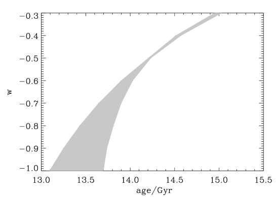
Figure 1: The region of parameter space allowed if we fix $\theta_{A}$ (which in turns fixes the position of the first CMB acoustic peak) and $\omega_{b}\equiv\Omega_{b}h^{2}=0.02$, weakly constraining $0.05<\Omega_{m}<0.45$ and $0.5<h<0.9$.

The ages of the oldest globular clusters (GCs) provide a lower limit to the total age of the universe. Since numerous star-forming galaxies have now been observed up to redshift $z=6.6$ (e.g., Kodaira et al., 2003)and the oldest GCs contain the oldest stellar populations in galaxies, it is reasonable to assume that GCs too have formed at redshift $z>6$. Krauss and Chaboyer (2003) perform the most careful analysis to date of the effects of systematics in GC age determinations. They estimate the age of the oldest Galactic GCs using the main-sequence turn-off luminosity and evaluate the errors with Monte-Carlo techniques, paying careful attention to uncertainties in the distance, to systematics, and to model uncertainties. They find a best-fit age for the oldest Galactic GCs of $12.5^{+3.4}_{-2.2}$ Gyr (95% confidence limits). We find that their probability distribution for the oldest GC age, can be accurately described by

$$P(t)=\frac{A}{\sigma(t-T)}\exp\left[-\frac{\ln\left[(t-T)/m\right]^{2}}{2\sigma^{2}}\right]$$ (5)

where $t$ denotes the age of the oldest GCs, $A=1.466$, $\sigma=0.25$, $T=6.5$ and $m=5.9$. Since the oldest GCs likely formed at $z>5$, for all reasonable cosmologies we only need add about $0.3$ Gyr to the GC ages to obtain an estimate of the age of the universe. Only the oldest (low metallicity) GCs should be used in the age estimate, for which there is no age spread (see e.g. Rosenberg et al. (1999), which finds no age spread for GCs with metallicities $[Fe/H]<-1.2$).

In order to constrain $w$, we can now assume a flat universe and Monte Carlo simulate the distribution of $\ell_{1}$ subject to only weak priors on the other cosmological parameters. For different values of $w$, Jimenez et al. (2003) generated $10^{5}$ models, randomly sampling the cosmological parameters $\Omega_{m}$, $\Omega_{b}h^{2}$ and $h$ with uniform priors, $0.5<h<0.9$, $0.05<\Omega_{m}<0.45$, and $0.01<\Omega_{b}h^{2}<0.03$. The next step is to impose an age of the universe constraint by randomly sampling these models so that the age of the universe has a probability distribution whose shape is given by equation 5, but offset by $0.3$ Gyr. Jimenez et al. (2003) used the publicly available code CMBFAST (Seljak and Zaldarriaga, 1996) to compute the resulting distribution of $\ell_{1}$. This is shown in Figure 2 where the two solid lines are the 68% and 90% joint confidence levels.

As expected, the age alone does not constrain $w$; there is a degeneracy between $w$ and $\ell_{1}$. If we now use the observed position of the first acoustic peak as recently measured, in a model independent way, from WMAP (Page et al., 2003), we can constrain $w$ with high accuracy. The filled contours in Figure 2 are marginalized values for $w$ at the 68% and 90% confidence levels. Thus we find $w<-0.8$ ($w<-0.67$) at the 68% (90%) confidence level.

This determination depends solely on the GC determination of the age of the universe and on the observed position of the first acoustic peak in the CMB power spectrum. This constraint is slightly less stringent than that obtained by Spergel et al. (2003) from a joint likelihood analysis of WMAP with six external data sets (WMAP + CBI + ACBAR + 2dFGRS + Lyman$\alpha$ forest power spectrum + Type Ia supernovae + $H_{0}$ constraint from the HST key project), but is tighter than the CMB-only (WMAP + CBI + ACBAR) determination and comparable to the WMAP + ACBAR + CBI + HST constraint.

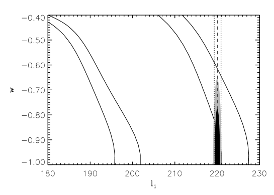
Figure 2: Confidence regions (68 and 90%) for the value of $w$ are shown by the filled grey areas (marginalized over the position of the first acoustic peak in the CMB, $\ell_{1}$). The solid lines denote contours which show the constraints in $w$ using the derived age of the oldest Galactic globular clusters only. The dash and dotted lines are the the position of the first acoustic peak and confidence region as measured by WMAP. Note that the position of the first peak greatly constrains the value of $w$.

3 Measuring a variable equation of state for the dark energy

The popular approach for measuring $w(z)$ uses its effect on the luminosity distance of sources. In particular, the proposal for the Supernova/Acceleration Probe (SNAP) mission suggests to monitor $\sim 2000$ Type Ia supernovae across the sky per year and determine their luminosity distances up to a redshift $z\sim 1.5$ with high precision. However, the sensitivity of the luminosity distance to the redshift evolution of $w(z)$ is compromised by its integral nature (Maor et al. 2001),

$$d_{\rm L}=(1+z)\int_{z}^{0}(1+z^{\prime}){dt\over dz^{\prime}}dz^{\prime},$$ (6)

where $t(z)$ is the age of the Universe at a redshift $z$ which depends on $w(z)$.

Jimenez and Loeb (2002) proposed an alternative method that offers a much better sensitivity to $w(z)$ since it measures the integrand of equation (6) directly. Any such method must rely on a clock that dates the variation in the age of the Universe with redshift. The clock is provided by spectroscopic dating of galaxy ages. Based on measurements of the age difference, $\Delta t$, between two passively–evolving galaxies that formed at the same time but are separated by a small redshift interval $\Delta z$, one can infer the derivative, $(dz/dt)$, from the ratio $(\Delta z/\Delta t)$. The statistical significance of the measurement can be improved by selecting fair samples of passively–evolving galaxies at the two redshifts and by comparing the upper cut-off in their age distributions. All selected galaxies need to have similar metallicities and low star formation rates (i.e. a red color), so that the average age of their stars would far exceed the age difference between the two galaxy samples, $\Delta t$.

This differential age method is much more reliable than a method based on an absolute age determination for galaxies (e.g., Dunlop et al. 1996; Alcaniz & Lima 2001; Stockton 2001). As demonstrated in the case of globular clusters, absolute stellar ages are more vulnerable to systematic uncertainties than relative ages (Stetson, Vandenberg & Bolte 1996). Moreover, absolute galaxy ages can only provide a lower limit to the age of the Universe and only place weak constraints on the possible histories of $w(z)$.

Consider a flat universe composed of matter and dark energy with an equation of state $p_{Q}=w(z)\rho_{Q}$. The Hubble parameter is $H^{2}=H_{0}^{2}[\rho_{T}(z)/\rho_{T}(0)]$. Here, the subscripts $Q$, $m$, and $T$ refer to the dark energy, the matter, or the total sum of the two, respectively. Assuming further that the matter is non-relativistic (i.e. effectively pressureless), we get

$$H_{0}^{-1}{dz\over dt}=-(1+z)^{5/2}\left[\Omega_{m}(0)+\Omega_{Q}(0)\exp\left\{3\int_{0}^{z}\frac{dz^{\prime}}{(1+z^{\prime})}w(z)\right\}\right]^{1/2},$$ (7)

where we have used the energy conservation equation for the dark energy, $\dot{\rho}_{Q}=-3H(1+w(z))\rho_{Q}$ (Maor et al. 2000). Thus, $({dz}/{dt})$ is related to the equation of state of the dark energy through one integration only, while the luminosity distance in equation (6) is given by an integral of the inverse of equation (7), namely through two integrations. By differentiating $(dz/dt)$ with respect to $t$ we find,

$$H_{0}^{-2}\frac{d^{2}z}{dt^{2}}=\frac{[H_{0}^{-1}({dz}/{dt})]^{2}}{(1+z)}\left[\frac{5}{2}+\frac{3}{2}w(z)\right]-\frac{3}{2}\Omega_{m}(0)(1+z)^{4}w(z),$$ (8)

which depends explicitly on $w(z)$ without any integrations. Thus, the second derivative of redshift with respect to cosmic time measures $w(z)$ directly. While it is possible to find significantly different redshift histories of $w(z)$ for which the evolution of $d_{\rm L}$ is similar, this cannot be done for $({d^{2}z}/{dt^{2}})$.

To obtain $dz/dt$, Jimenez and Loeb (2002) proposed to use the old envelope of the age–redshift relation of E/S0 galaxies. They assume that E/S0 at different redshifts are drawn from the same parent population with the bulk of their stellar populations formed at relatively high redshift (e.g., Bower et al., 1992; Stanford et al., 1998). Then, at relatively low redshift, they are evolving passively and may be used as “cosmic chronometers”.

Recently, Jimenez et al. (2003) applied this method using high-quality spectra of a sample of old stellar populations covering the largest possible range in redshift. To this aim they combined the following data sets: (i) the luminous red galaxy (LRG) sample from the Sloan Digital Sky Survey (SDSS) early data release (Eisenstein et al., 2001); (ii) the sample of field early-type galaxies from Treu et al. (1999, 2001, 2002, hereafter the Treu et al. sample); (iii) a sample of red galaxies in the galaxy cluster MS1054$-$0321 at $z=0.83$; and (iv) the two radio galaxies 53W091 and 53W069 (Dunlop et al., 1996; Spinrad et al., 1997; Nolan et al., 2003, Dey et al., in preparation). They obtained the age of the dominant stellar population in the galaxies by fitting single stellar population models (Jimenez et al., 1998) to the observed spectrum.

Figure 3: Top panel: Age–redshift envelope obtained for the galaxies studied in Jimenez et al. (2003). Open circles correspond to galaxies from the SDSS LRG sample, triangles to the Treu et al. sample, diamonds to MS1054$-$0321, and crosses are 53W091 and 53W069. A clear trend is present: galaxies age as the redshift decreases. The overall shape of this trend is in fair agreement with theoretical expectations for a $\Lambda$CDM (solid line) with $\Omega_{m}=0.27$ and $H_{0}=71$ km s^-1 Mpc^-1. The dotted line represent an alternative model disfavored by the data: $w(z)=-2$ for $z>1$ and then grows linearly from $w=-2$ at $z=1$ to $w=0$ at $z=0$. Bottom panel: histogram along the age axis of top panel for the redshift range $0<z<0.04$ and $0.08<z<0.12$. The clear shift between the two histograms is a measurement of $dz/dt$ and therefore allows us to measure $H_{0}$.

Figure 3 shows the derived single-burst equivalent ages of the galaxies as a function of redshift. The circles correspond to galaxies in the SDSS LRG sample, triangles refer to the Treu et al. sample, diamonds are galaxies in MS1054$-$0321, and crosses are 53W091 and 53W069. For clarity, the SDSS LRG points have not been plotted for ages $<7$ Gyr. Typical errors on the ages of LRG galaxies are 10% and are not plotted. An age–redshift relation (i.e., an “edge” or “envelope” of the galaxy distribution in the age–redshift plane) is apparent from $z=0$ to $z=1.5$. Jimenez et al. (2003) also show that small recent episodes of start formation do not significantly bias the age determination.

What are the observational limits that can be imposed on $w(z)$? As a consistency check we note that the age at $z=0$ obtained with this method is in good agreement with GC ages and that the Treu et al. galaxy ages agree with those from of SDSS LRG sample where they overlap. The solid line in Figure 3 corresponds to the age–redshift relation for a flat, reference $\Lambda$CDM model: $\Omega_{m}=0.27$, $h=71$, and $w=-1$ (WMAP best fit model). This is consistent with the observed age–redshift envelope, and it seems to indicate that we live in a universe with a classical vacuum energy density and that, on average, stars in the oldest galaxies formed about 0.7 Gyr after the Big Bang (e.g., at redshifts $z\sim 7-10$). To make the observed age–redshift relation consistent with a model with widely different $w(z)$ behavior, one would have to infer that early-type galaxies at different redshifts have very different formation epochs for their stellar populations. For example, the dotted line in Figure 3 indicates the age-redshift relation for a passively evolving population in a universe where $w(z)=-2$ for $z>1$ and grows linearly from $w=-2$ at $z=1$ to $w=0$ at $z=0$. For this model to work, we would have to conclude that the oldest galaxies at $z\sim 1.5$ formed about 0.7 Gyr after the Big Bang, but that the oldest galaxies at $z\sim 0$ formed $\sim 3$ Gyr after the Big Bang. Since the oldest galaxies in the LRG sample are as old as the oldest GCs, we consider this to be an unlikely explanation. Furthermore, not only would this scenario require that all local galaxies either formed their stars more recently than galaxies at high redshift or had recent episodes of star formation, but would also require a remarkable fine-tuning for them all to end up with exactly the same age. We therefore conclude that this extreme model for $w(z)$ is unlikely given the data.

Unfortunately, the small number of galaxies in Jimenez et al. (2003) samples at $z>0.2$ did not allow them to compute $dz/dt$ with enough accuracy to constrain $w(z)$, and therefore this measurement will have to await better data. However, the $z<0.2$ region is well populated by LRG galaxies (Figure 3) and they determined $dt/dz$ at $z\sim 0$. This is illustrated in the bottom panel of Figure 3 by the clear shift in the upper envelope of the age histogram between the two redshift ranges $0<z<0.04$ and $0.08<z<0.12$. This can be used to determine $H_{0}$, which relies upon determining the “edge” of the galaxy age distribution in different redshift intervals.

If the ages of the galaxies were known with infinite accuracy, for each galaxy_i at redshift $z_{i}$, one could associate an age $a_{i}$. The probability for the age of the oldest stellar population in galaxy_i, $P(t|a_{i})$, would be given by a step function which jumps from 0 to 1 at $a_{i}$. An age–redshift relation edge could then be obtained by dividing the galaxy sample into suitably-large redshift bins and multiplying the $P(t|a_{i})$ for all the galaxies in each bin.

Figure 4: The binned, low-redshift age–redshift relation, derived from the SDSS LRG sample. The solid line is a best-fit to the edge.

In practice, the age of each galaxy is measured with some error $\delta a_{i}$. We thus assume $P(t|a_{i})=1$ if $t>a_{i}+\delta_{a_{i}}$ and $\ln P(a_{i})=-x^{2}$ where $x=(a_{i}+\delta_{a_{i}}-t)/(\sqrt{2}\delta_{a_{i}})$ otherwise. Jimenez et al. (2003) divided the $z<0.2$ portion of the LRG sample into 51 redshift bins. For each bin, they obtained $P(z,t)$ by multiplying the $P(t|a_{i})$ of the galaxies in that bin. They define the “edge” of the distribution $t(z)$ to be where $\ln P(z,t)$ drops by $0.5$ from its maximum (i.e. $\Delta\ln P=0.5$ and associate an error to this determination $\delta_{t(z)}$ given by $t_{2}(z)-t(z)$ where $t_{2}(z)$ corresponds to where $\ln P(z,t)$ drops by $2$ from its maximum (i.e. $\Delta\ln P=2$, this approximately corresponds to the 68% confidence level). This procedure makes the determination of the “edge” less sensitive to the outliers (see also Raychaudhury et al. (1997)). Figure 4 presents the resulting $t(z)$ relation.

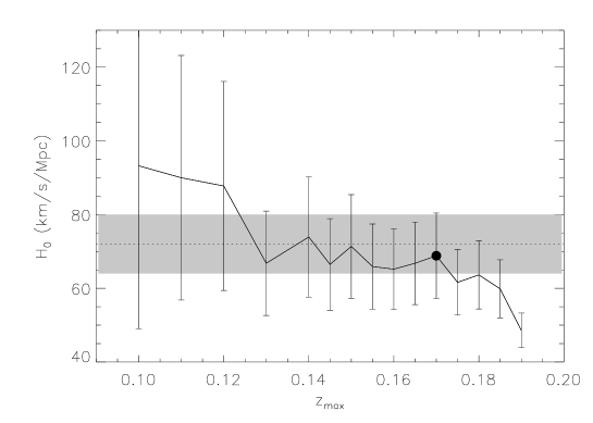
Figure 5: The value for $H_{0}$ derived from Figure 4 as a function of redshift cut-off for computing the slope. Note that it is very weakly dependent on the value of this cut-off. The solid circle is the adopted value. The shaded are corresponds to the 1$\sigma$ confidence region from the Hubble Key Project. For $z>0.18$ the probability of the fit being a straight line is $P_{\geq\chi^{2}}<0.1$, while at $z=0.17$ is 0.32.

For $z<z_{\rm max}$, Jimenez et al. (2003) fit $t(z)$ with a straight line whose slope $dt/dz$ is related to the Hubble constant at an effective redshift by $H(z_{\rm eff})=-\frac{1}{1+z_{\rm eff}}(\frac{dt}{dz})^{-1}$. This fit is performed by standard $\chi^{2}$ minimization. They also compute $P_{\geq\chi^{2}}$, the probability of obtaining equal or greater value of the reduced $\chi^{2}$ if the $t(z)$ points were truly lying on a straight line. Values of $P_{\geq\chi^{2}}<0.1$ means that a straight line is not a good fit to the points.

For $w=-1$, $H_{0}=H(z_{\rm eff})\left[\Omega_{m}(1+z_{\rm eff})^{3}+\Omega_{\Lambda}\right]^{-\frac{1}{2}}$ where $\Omega_{m}=0.27$, $\Omega_{\Lambda}=0.7$. Figure 5 shows how the $H_{0}$ measurement depends on $z_{\rm max}$. For $z_{\rm max}>0.17$ not only the value for $H_{0}$ drifts but also a straight line is not a good fit to the points ($P_{\geq\chi^{2}}$ suddenly drops below $0.1$). For their $H_{0}$ determination, $z_{\rm max}=0.17$, $P_{\geq\chi^{2}}=0.32$, $z_{\rm eff}=0.09$, and the correction from $H(z_{\rm eff})$ to $H_{0}$ is a $4\%$ effect. They obtained $H_{0}=69\pm 12$ km s^-1 Mpc^-1. Which is in good agreement with the Hubble Key Project measurement ($h=0.72\pm 0.03\pm 0.07$; Freedman et al., 2001), with the valued derived from the joint likelihood analysis of WMAP + 2dFGRS + Lyman-$\alpha$ forest power spectrum ($h=0.71^{+0.04}_{-0.08}$; Spergel et al., 2003), with gravitational lens time delay determinations ($h=0.59^{+0.12}_{-0.07}\pm 0.03$; Treu and Koopmans, 2002), and Sunyaev-Zeldovich measurements ($h=0.60^{+0.04+0.13}_{0.04-0.18}$; Reese et al., 2002).

This check at $z=0$ gives some confidence about the possibility of measuring $w(z)$ when larger samples of elliptical galaxies at higher redshifts become available in the near future. DEEP2 and the full SDSS catalog will provide excellent datasets for doing this.

I warmly thank my collaborators Avi Loeb, Dan Stern, Tommaso Treu and Licia Verde.

References

- Alcock and Paczynski (1979) Alcock, C., Paczynski, B., 1979. Nature 281, 358.
- Baccigalupi et al. (2002) Baccigalupi, C., Balbi, A., Matarrese, S., Perrotta, F., Vittorio, N., 2002. PRD 65, 63520.
- Birkinshaw (1999) Birkinshaw, M., 1999. The Sunyaev-Zel’dovich Effect: an Update. In: AIP Conf. Proc. 476: 3K cosmology. pp. 298.
- Bower et al. (1992) Bower, R. G., Lucey, J. R., Ellis, R. S., 1992. MNRAS 254, 601.
- Caldwell et al. (2003) Caldwell, R., Kamionkowski, M., Weinberg, N., 2003. astro-ph/0305008.
- Caldwell et al. (1998) Caldwell, R. R., Dave, R., Steinhardt, P. J., 1998. PRD 80, 1582–1585.
- Dunlop et al. (1996) Dunlop, J., Peacock, J., Spinrad, H., Dey, A., Jimenez, R., Stern, D., Windhorst, R., 1996. Nature 381, 581–584.
- Efstathiou (1999) Efstathiou, G., 1999. MNRAS 310, 842–850.
- Eisenstein et al. (2001) Eisenstein et al., D. J., 2001. AJ 122, 2267–2280.
- Freedman et al. (2001) Freedman, W. L. et al., 2001. ApJ 553, 47–72.
- Garnavich et al. (1998) Garnavich et al., P. M., 1998. ApJ 509, 74.
- Haiman et al. (2001) Haiman, Z., Mohr, J. J., Holder, G. P., 2001. ApJ 553, 545–561.
- Hu (2002a) Hu, W., 2002a. PRD 66, 83515.
- Hu (2002b) Hu, W., 2002b. PRD 65, 23003.
- Hu et al. (2001) Hu, W., Fukugita, M., Zaldarriaga, M., Tegmark, M., 2001. ApJ 549, 669–680.
- Hui (1999) Hui, L., 1999. ApJL 519, L9–L12.
- Huterer (2002) Huterer, D., 2002. PRD 65, 63001.
- Huterer and Turner (2001) Huterer, D., Turner, M. S., 2001. PRD 64, 123527.
- Jimenez and Loeb (2002) Jimenez, R., Loeb, A., 2002. ApJ 573, 37–42.
- Jimenez et al. (1998) Jimenez, R., Padoan, P., Matteucci, F., Heavens, A. F., 1998. MNRAS 299, 123.
- Jimenez et al. (2003) Jimenez, R., Verde, L., Treu, T., Stern, D., 2003. astro-ph/0302560.
- Knox et al. (2001) Knox, L., Christensen, N., Skordis, C., 2001. ApJL 563, L95–L98.
- Kodaira et al. (2003) Kodaira et al., K., 2003. astro-ph/0301096.
- Krauss and Chaboyer (2003) Krauss, L. M., Chaboyer, B., 2003. Science 299, 65–70.
- Kujat et al. (2002) Kujat, J., Linn, A. M., Scherrer, R. J., Weinberg, D. H., 2002. ApJ 572, 1–14.
- Lima and Alcaniz (2002) Lima, J. A. S., Alcaniz, J. S., 2002. ApJ 566, 15–18.
- Newman and Davis (2000) Newman, J. A., Davis, M., 2000. ApJL 534, L11–L14.
- Nolan et al. (2003) Nolan, L., Dunlop, J., Jimenez, R., Heavens, A. F., 2003. MNRAS 341, 464.
- Page et al. (2003) Page et al., L., 2003. astro-ph/0302220.
- Perlmutter et al. (1999) Perlmutter et al., S., 1999. ApJ 517, 565–586.
- Raychaudhury et al. (1997) Raychaudhury, S., von Braun, K., Bernstein, G. M., Guhathakurta, P., 1997. AJ 113, 2046–2053.
- Reese et al. (2002) Reese, E. D., Carlstrom, J. E., Joy, M., Mohr, J. J., Grego, L., Holzapfel, W. L., 2002. ApJ 581, 53.
- Riess et al. (1998) Riess et al., A. G., 1998. AJ 116, 1009–1038.
- Rosenberg et al. (1999) Rosenberg, A., Saviane, I., Piotto, G., Aparicio, A., 1999. AJ 118, 2306–2320.
- Seljak and Zaldarriaga (1996) Seljak, U., Zaldarriaga, M., 1996. ApJ 469, 437.
- Spergel et al. (2003) Spergel et al., D., 2003. astro-ph/0302209.
- Spinrad et al. (1997) Spinrad, H., Dey, A., Stern, D., Dunlop, J., Peacock, J., Jimenez, R., Windhorst, 1997. ApJ 484, 581.
- Stanford et al. (1998) Stanford, S. A., Eisenhardt, P. R. M., Dickinson, M., 1998. ApJ 492, 461.
- Tonry et al. (2003) Tonry et al., J., 2003. astro-ph/0305008.
- Treu and Koopmans (2002) Treu, T., Koopmans, L. V. E., 2002. MNRAS 337, L6–L10.
- Treu et al. (1999) Treu, T., Stiavelli, M., Casertano, S., Møller, P., Bertin, G., 1999. MNRAS 308, 1037–1052.
- Treu et al. (2002) Treu, T., Stiavelli, M., Casertano, S., Møller, P., Bertin, G., 2002. ApJL 564, L13–L16.
- Treu et al. (2001) Treu, T., Stiavelli, M., Møller, P., Casertano, S., Bertin, G., 2001. MNRAS 326, 221.
- Turner and White (1997) Turner, M. S., White, M., 1997. PRD 56, 4439.
- Verde et al. (2003) Verde et al., L., 2003. astro-ph/0302218.
- Wang and Garnavich (2001) Wang, Y., Garnavich, P. M., 2001. ApJ 552, 445–451.
- Weller and Albrecht (2001) Weller, J., Albrecht, A., 2001. PRL 86, 1939–1942.