Secondary antiproton flux induced by cosmic ray interactions with the atmosphere

Abstract

The atmospheric secondary antiproton flux is studied for detection altitudes extending from sea level up to about 3 earth radii, by means of a 3-dimensional Monte-Carlo simulation, successfully applied previously on other satellite and balloon data. The calculated antiproton flux at mountain altitude is found in fair agreement with the recent BESS measurements. The flux obtained at balloon altitude is also in agreement with calculations performed in previous studies and used for the analysis of balloon data. The flux at sea level is found to be significant. The antineutron flux is also evaluated. The antiproton flux is prospectively explored up to around 2 10⁴ km. The results are discussed in the context of the forthcoming measurements by large acceptance experiments.

I Introduction

The antiproton ($\overline{p}$) has a particular status in the spectrum of Cosmic Radiation mainly because of its particular production dynamics and kinematics. The main part of the Cosmic Ray (CR) $\overline{p}\;$spectrum measured in balloon and satellite experiments is well accounted for by assuming it to consist of a secondary flux, originating from the interaction between the nuclear CR flux and the interstellar matter in the galaxy (ISM) DO01 . It is expected to be dominant with respect to components from other possible origins. Such other contributions of primary origin and of major astrophysical interest, have been considered recently. In particular, the $\overline{p}\;$flux induced by annihilation of dark matter constituents ST88 ; BO99a ; BE99 , and by primordial black hole evaporation CA76 ; BA00 have been discussed. All these possible contributions are intimately entangled together and their phenomenological disentagling relies critically on the accuracy of the experimental data. The measurements of the $\overline{p}\;$flux thus provide a sensitive test of the production source and mechanism, and of the propagation conditions in the galaxy DO01 ; GA92 ; CH97 ; SI98 ; BI99 ; UL99 ; MO02 .

CR antiprotons have been experimentally studied for several decades by satellite or balloon borne experiments (see references in BO01 ). Several recent balloon experiments, like BESS BESS97 ; BESS98 and CAPRICE BO01 ; BO97 have collected new data samples whose analysis have provided determinations of the galactic $\overline{p}\;$flux over a kinetic energy range extending from about 0.2 GeV kinetic energy up to about 50 GeV. In these works, the values of the antiproton galactic flux were obtained by subtracting the calculated atmospheric $\overline{p}\;$flux from the values of the measured total flux.

Secondary galactic as well as atmospheric antiprotons are both produced in hadronic collisions by the same elementary reaction mechanism in nucleon-nucleon collisions between the incident CR flux and either ISM nuclei (mainly Hydrogen) in the galaxy, or atmospheric nuclei (mainly Nitrogen) in the atmosphere. The basic $\overline{p}\;$production reaction is the inclusive $NN\rightarrow\bar{p}X$ process, $N$ standing for nucleon and X for any final quantal hadronic state allowed in the process. The ratio of $\overline{p}\;$production in the galaxy and in the atmosphere scales with the ratio of matter thickness (in units of interaction length $\lambda_{I}$) crossed by protons in the two media. These thicknesses are known to be of the same order of magnitude. In addition, both flux are driven by similar transport equations (see GA92 ; SI98 ; PF96 ; GA99 for example), with however the escape term arising from convective and diffusive effects in the interstellar medium on the galactic flux GA92 , making a significant difference with the transport of flux in atmosphere, which tends to decrease the transported flux compared to the atmospheric transport conditions.

It can be shown using a Leaky Box Model (LBM) for the galactic transport and a simple slab model for the production in the upper atmosphere MA01 , that the ratio of the atmospheric $\overline{p}\;$flux at balloon altitude $N_{atm}$ to the galactic $\overline{p}\;$flux at TOA $N_{gal}$, is approximately:

$$\frac{N_{atm}(\bar{p})}{N_{gal}(\bar{p})}\approx\frac{x_{Atm}}{\lambda_{e}}\frac{\sigma(p\,Atm\rightarrow\bar{p}X)}{\sigma(pp\rightarrow\bar{p}X)}\frac{m_{H}}{m_{Atm}}\approx\frac{x_{Atm}}{\lambda_{e}}(\frac{m_{H}}{m_{Atm}})^{1/3}$$

Where $x_{Atm}$ is the thickness of atmosphere on top of balloon experiments, while $\lambda_{e}$ is the LBM escape length, $\sigma(pp\rightarrow\bar{p}X)$ and $\sigma(p\,Atm\rightarrow\bar{p}X)$ being the inclusive antiproton production cross sections on hydrogen and on the atmospheric nuclei respectively, while $m_{H}$ and $m_{Atm}$ are the hydrogen and the mean atmospheric nuclear mass respectively. Using $x_{Atm}$=3.9 g/cm² (for a 38 km altitude) HE91 and $\lambda_{e}$=8 g/cm² and 11.8 g/cm² for particle rigidities of 3 GV and 10 GV respectively MATT , the above ratio is found to be of the order of 0.15 and 0.2, respectively. The contribution of the atmospheric antiproton production to the total flux measured in balloon experiments is thus not expected to be negligible with respect to the galactic component. The correction of the total flux from the atmospheric contribution therefore needs the latter to be calculated very carefully since the accuracy on the evaluation of this component sets a limit of accuracy on the final value of the measured galactic flux.

It must be emphasized that studying also the secondary proton flux in the atmosphere in this context is interesting since the latter is very sensitive to all the components of the simulation process, in particular to the secondary proton production cross section which contributes as well to the generation of the antiproton flux. The comparison of the calculation to the recently measured data provides a robust validation of the approach used and of the overall calculation, and firmly supports the reliability of the results reported here. This study is reported in a separate (companion) paper BA03 .

The present work is an extension of a resarch program aiming at the interpretation of satellite data and which first results on the flux of protons, leptons, and light ions, below the geomagnetic cutoff (GC), at satellite altitude, have been reported recently PAP1 ; PAP2 ; PAP3 .

The paper reports on the calculated $\overline{p}\;$atmospheric flux over the range from sea level up to satellite altitudes by Monte-Carlo simulation. The main features of the calculations are described in section II. The production cross sections used in the event generator are given in section III. The results are discussed in section IV. The work is concluded in section V.

II Simulation conditions

As mentioned above, the flux of secondary atmospheric antiprotons has been investigated using the same simulation approach which has allowed to successfully account for the $p$, $d$, $H\!e$, and $e^{\pm}$ experimental flux below the Geomagnetic Cutoff (GC) measured by the AMS experiment, as well as the experimental proton and muon flux in the atmosphere, the latter being studied together with the atmospheric neutrino flux LI03 .

The same computing environment has been used here for the charged particle propagation in the terrestrial environment including the atmosphere, as in the previous studies, with the event generator being dedicated however, based on the antiproton production cross section in nucleon-nucleon collisions.

The calculation proceeds by means of a full 3D-simulation program. Incident Cosmic Rays are generated on a virtual sphere chosen at a 2000 km altitude. Random events are generated uniformly on this sphere. The local zenith angle distribution of the particule momentum is proportional to $\cos(\theta_{z})d\cos(\theta_{z})$, $\theta_{z}$ being the zenithal angle of the particle, in order to get an isotropic flux at any point inside the volume of the virtual sphere. The geomagnetic cut-off is applied by back-tracing the particle trajectory in the geomagnetic field, and keeping in the sample only those particles reaching a backtracing distance of 10 Earth radii. Flux conservation along any allowed particle path in the geomagnetic field is ensured by application of Liouville’s theorem. The normal particle propagation as well as its back-tracing are performed using the adaptative Runge-Kutta integration method in the Geomagnetic field LI03 .

1. For the incident CR proton and helium flux, functional forms fitted to the 1998 AMS measurements were used PROT ; HELI (see also BO99 ; ME00 ; SA00 ). The heavier components of the CR flux were not taken into account in the calculations (see LI03 ). For other periods of the solar cycle, the incident cosmic flux are corrected for the different solar modulation effects using a simple force law approximation SOLMOD .

2. Each particle is propagated in the geomagnetic field and interacts with nuclei of the local atmospheric density according to their total reaction cross section and producing secondary nucleons $p$, $n$, and antinucleons $\overline{p}\;$, $\overline{n}\;$, with cross sections and multiplicities. This important issue is discussed in section III below. The specific ionization energy loss is computed for each step along the trajectory.

3. In the following step, each secondary particle produced in a primary collision is propagated in the same conditions as incident CRs in the previous step, resulting in a more or less extended cascade of collisions through the atmosphere, which may include up to ten generations of secondaries for protons for the sample generated in this work BA03 ; PAP1 .

For the antinucleon inelastic collisions, only the annihilation reaction channel was taken into account. Non annihilating inelastic $\bar{N}+A\rightarrow\bar{N}+X$ ($\bar{N}$ standing for antinucleon) interactions whose contribution to the total reaction cross section $\sigma_{R}$, is small. It consists basically of the single diffractive dissociation cross section (for the proton target in individual $\bar{N}p$ collisions), and it would be of the same order of magnitude as for pp colisions, namely $\sim$10% of $\sigma_{R}$ or less at the energies considered here PBARINEL . It has been neglected at this stage. It will be included in the further developments of the calculation program.

The reaction products are counted whenever they cross, upwards or downwards, the virtual detection spheres (several can be defined in the program) at the altitude of the detectors: from sea level up to about 36 km for ground and balloon experiments (BESS, CAPRICE), 370 km for the AMS satellite experiment. Higher altitudes up to more than 10000 km were also investigated, with the purpose of understanding the dynamics of the population of quasi-trapped particles in the earth environment (see section IV.7). Each particle is propagated until it disappears by nuclear collision (annihilation for antinucleons), stopping in the atmosphere by energy loss, or escaping to the outer space beyond twice the generation altitude PAP1 ; PAP2 ; PAP3 ; LI03 .

In the terminology used in the following, one event is defined as the full cascade induced by an incoming CR particle interacting with one atmospheric nucleus. For each CR producing at least one secondary particle, the whole event is stored with all the relevant topological, dynamical, kinematical, and geographical informations. This includes the collision rank, geophysical location, altitude, momentum and particle type, and parent particle type, in form of event files. The collision rank is defined as the number of a given collision in the cascade initiated by the first CR interaction with atmosphere (rank 1).

The calculations do not include any adjustable parameter.

III Cross sections

III.1 Proton induced secondaries

III.1.1 Protons

The inclusive $p+A\rightarrow p+X$ proton production cross sections used are described in ref PAP1 . They are based on the results of refs BA85 and AB92 for the two components corresponding basically to forward (or direct quasi elastic) and backward (or relaxed deep inelastic) productions respectively. The values obtained have been found in reasonable agreement with the results of the INCL model of intranuclear cascade calculations BO02 . This cross section allows to reproduce very successfully the atmospheric secondary proton flux down to the lowest altitude BA03 .

The cross section for secondary neutron production was taken equal to that of proton production. Similarly, the neutron induced cross sections of secondary nucleon production used was taken the same as for protons, the coulomb interaction making negligible differences over the considered energy range.

III.1.2 Antiprotons

The inclusive $p+A\rightarrow\bar{p}+X$ antiproton production cross section has been obtained by fitting a set of available experimental data between 12 GeV incident kinetic energy and 24 GeV/c incident momentum SU98 ; AB93 ; AL70 ; EI72 , using a modified version of the analytical formula proposed in ref KMN , the latter being referred to as KMN (for Kalinovski, Mokhov, Nikitin) in the following.

The invariant triple differential cross section is described by means of the formula used in KMN :

$$(E\frac{d^{3}\sigma}{d^{3}p})_{inv}=\sigma_{R}C_{1}A^{b(p_{t})}(1-x)^{C_{2}}\exp(-C_{3}x)\Phi(p_{t})\\$$ (1)

In this relation the kinematical variables $p_{t}$ and $x$ are the transverse momentum and the fractional energy of the particle respectively as defined in KMN (relation 3.26 in this reference), while $\sigma_{R}$ is the total $p+A$ reaction cross section. The function $\Phi(p_{t})$ was modified as:

$$\Phi(p_{t})=\exp(-C_{4}p_{t}^{2})+C_{5}\frac{\exp(-C_{6}x_{t})}{(p_{t}^{2}+\mu^{2})^{4}}\exp(-\alpha\sqrt{s})$$ (2)

With $b(p_{t})=b_{0}\cdot p_{t}$ within the range of 4-momentum transfer considered here. Figure 1 shows some of the results obtained HU01a by fitting the set of available data studied for this work with relation 1. The energy dependent exponential factor in the second term of relation 2 was introduced for it was found that this term contributes only at low incident energy. The values of the parameters obtained are given in table 1. These values are significantly different from those given in the original work HU01a ; HU02 on a smaller number of data. This work is currently being extended up to 400 GeV incident proton energy DU03 .

Table 1: Values of the parameters of relation 1 obtained in fitting the data of figure 1.

Parameter	$C_{1}$	$C_{2}$	$C_{3}$	$C_{4}$	$C_{5}$	$C_{6}$	$\mu$	$b_{0}$	$\alpha$
value	0.042	5.92	0.96	2.19	84.3	10.5	1.1	0.12	2.24

Figure 1: Sample of the fits to the $p+A\rightarrow\bar{p}+X$ cross section data using the parametrized relation 1 given in the text, with the parameters of table 1 HU01a . Top left: Differential cross sections measured at 5.1^∘ for $p+C$ (full squares) and for $p+Al$ (full circles) SU98 as a function of the particle momentum, compared with fit using 1 (thick solid for $Al$ and thick dashed for $C$), and using the KMN relation and parameters from KMN (thin solid and thin dashed resp.). Top right: Same comparison for 14.6 GeV/c $p+Al$ invariant differential cross section versus mass transfer from AB93 : Fit with 1 (thick line) and KMN calculations KMN (thin line). Bottom left: Same for 19.2 GeV/c $p+p$ (full squares) and $p+Al$ (full circles) rapidity distributions from AL70 : fit with 1 (solid and dashed thick lines resp.) and KMN calculations KMN (thin solid and dased lines resp.). Bottom right: 24 GeV/c $p+Al$ invariant differential cross sections at various angles (in msr on the figure) from EI72 compared to the fits with 1. For each measurement angle above the first (17 mrad), each next cross section has been multiplied by 10^-1,-2,… for presentation purpose. KMN calculations are not shown on this figure for legibility. Note that the same definitions of cross sections have been used as in the original references. There is a clear target mass dependence of the differential cross section in the top left panel, while in the bottom left panel almost no such dependence is observed, because the observable displayed is a multiplicity, i.e., ratio of differential cross section to total reaction cross section.

III.2 ⁴He induced secondaries

III.2.1 Protons

The inclusive ${}^{4}He+A\rightarrow p(n)+X$ proton (neutron) production cross section was obtained as described in section III.1.1 above for the $p+A\rightarrow p+X$ cross section (using the total reaction cross section from JA78 for this system), renormalized to the available experimental multiplicities measured for this reaction AR87 ; BA93 .

III.2.2 Antiprotons

The inclusive antiproton production cross section was evaluated by means of the wounded nucleon model BI76 ; FA84 using the experimental values of the total reaction cross sections for the ${}^{4}He+A$ and $p+A$ systems, and of the $\overline{p}\;$production multiplicity in nucleon-nucleon collisions HU02 available.

In this model, the particle production multiplicity $<n_{AB}>$ in the collision between ions $A$ and $B$ is related to the multiplicity nucleon-nucleon ${\cal(NN)}$ collision $<n_{\cal NN}>$ by the relation:

$$<n_{AB}>~{}=~{}\frac{1}{2}\left(A\frac{\sigma_{pB}}{\sigma_{AB}}+B\frac{\sigma_{pA}}{\sigma_{AB}}\right)<n_{\cal NN}>$$ (3)

with $\sigma_{ij}$ being the total reaction cross section between the $i$ and $j$ system. Using this model, the $\overline{p}\;$production multiplicity induced by the CR $He$ component on the nitrogen $N$ component of the atmosphere is found to be $<n_{HeN}>\approx 1.55<n_{pN}>\approx 2.5<n_{PP}>$.

III.3 Total reaction cross sections

$\bullet\;$Protons: The values of the proton total reaction cross section on nuclei used were obtained from the parametrization of LE83 , and checked on the carbon data from JA78 .
$\bullet\;$⁴He: The ⁴He+A total reaction cross sections used were taken from JA78 .
$\bullet\;$Antinucleons: The $\overline{p}\;$total reaction cross section was taken from CA79 , with the energy dependence from the data compilation of BA88 . The same production cross section and total reaction cross section have been assumed for $\overline{n}\;$production as for $\overline{p}\;$.

IV RESULTS

A sample of about 35 10⁶ CRs have been simulated, of which 20% were effectively propagated to the atmosphere (above GC), for detection altitudes going from sea level up to 10⁴ km altitude, including the BESS/CAPRICE balloon altitude ($\approx$38 km), the AMS orbit altitude ($\approx$370 km), and the recent BESS measurement terrestrial altitude (2770 m). The flux at sea level was calculated to investigate the possibility of ground level measurement of atmospheric antiprotons with existing devices HU01b . This was achieved independently by BESS at mountain altitude and the results are discussed below.

IV.1 Particle trajectories in the Earth magnetic field

Figure 2: Examples of antiproton trajectories in the earth magnetic field. Details are discussed in the text.

The time of confinement of particles in the earth environment together with their particular trajectories, determine their status with respect to the three categories: trapped, semi-trapped, and non trapped (escape). Trapped particles are spiralling back and forth around and along the magnetic field lines long enough to drift many times around the earth (see for example SI62 ; ST55 and below). Trapped particles are practically not observed in the energy domain considered here. They are not dynamically forbiden however and a few trajectories with a few 10² bounces are observed, which corresponds to short-lived trapped particles. Quasi trapped particles are in similar kinematic conditions but accomplish only a limited number of bounces at mirror points before being absorbed or before escaping (see examples below). This concept appeared during the first years of radiation belts studies GA60 (see also the discussion in SI62 ). Escape particles do not match the kinematic conditions for being trapped at their production point and escape in a very short time to the outer space. All intermediate situations between the stereotypes of quasi-trapped and escape trajectories are in fact observed in the simulation results (see example in bottom left fig 2).

Figure 2 shows four examples of characteristic trajectories of antiprotons generated in this study. Each of the 4 panels gives a side view (projection on the meridian plane, top left), side view zoomed around the production point showing the spiralling trajectory of the particle (top right), top view (projection on the equatorial plane, bottom left), and 3-D representation (bottom right) of each of the selected trajectories.

The top left event (1.52 GeV kinetic energy) is an escape particle produced close to the North pole. Top right is a semi trapped single bounce event (0.54 GeV) annihilating in the atmosphere close to its production point. Bottom left is a longer lifetime, multi bounces, semi trapped event (2.48 GeV), drifting around the earth about three quarters of a turn before annihilation in the atmosphere in the SAA region. Bottom right is intermediate between semi-trapped (since it displays at least one clear bounce) and escape event (0.54 GeV). It is a type of event for which the first adiabatic invariant (magnetic moment conservation) is not conserved because of a large variation of the magnetic field along the radius of gyration SI62 .

IV.2 General features of the simulated data

Figure 3 shows a few basic distributions of physics observables relevant to the dynamics of the process for two detection altitudes: 38 km (solid line) and 380 km (dashed line) corresponding to balloon and satellite (AMS) altitudes, inside and outside the atmosphere, respectively. The rank of the collision producing the antiproton (top left panel on the figure) appears to extend from 1 up to about 10 for the simulated sample, showing that $\overline{p}$s are produced up to the tenth generation in the collisions cascade. The distributions are a little different for the two altitudes, with a significantly larger number of $\overline{p}\;$occuring from first interaction at the lower altitude. The altitude distribution of the production point for the detection at 38 km (top right) shows a discontinuity at this altitude due to the incoming flux dominated by production from the upper layer of atmosphere. The mean production altitude is found around 46 km and 48 km for the lower and upper detection altitudes respectively. The particle momentum spectrum at the production point (bottom left) is found harder at the higher altitude. The number of bounces at the mirror points for particle trajectories spiralling around the magnetic field lines are found as expected very different for the two altitudes of detection: At 38 km, only a small population is seen to reach a number of bounces larger than a few units (5-6). This flux is significant however and must correspond to trajectories lying mostly outside of the atmosphere. At 380 km, the observed flux of $\overline{p}\;$ trajectories with more than one bounce is larger by about 2 orders of magnitude than at 38 km, corresponding to the population of quasi-trapped particles as discussed previously in PAP1 ; BU01 .

Figure 3: General features of the simulated $\overline{p}\;$sample at ballon (38 km) and satellite (380 km) altitude. Top left: Rank distribution (see text); Top right: Altitudes of production; Bottom left: Momentum distributions; Bottom right: Numbers of bounces effected by the particle between the mirror points. The spikes observed for high bounce multiplicity in this distribution correspond to quasi trapped particles trajectories crossing many times the detection altitude.

IV.3 Antiproton flux at mountain altitude

Figure 4: Antiproton flux data at 2770 m measured by BESS FU01 (symbols) compared with simulation results (histograms). Thick histogram: full calculation; Thin histogram: CR ⁴He contribution; dotted line: transport equation calculation from ST97 .

Figure 5: Experimental zenith angle distribution of the antiproton flux at 2770 m in bins of kinetic energy compared with simulation results.

The recent measurements of the $\overline{p}\;$flux at 2770 m of altitude by the BESS collaboration FU01 allows a sensitive test of the ability of the present simulation program to account for the observed flux since at this altitude the $\overline{p}\;$production occurs on the average after a casade of 4 collisions on the average (see previous section and fig 3). Another highly sensitive test of the overall calculation is provided in BA03 on the atmospheric proton flux.

Figure 5 shows the $\overline{p}\;$spectrum at 2770 m of altitude measured by BESS, compared to the simulation results. The latter has been run with the geometrical acceptance function of the BESS spectrometer given in FU01 (figures 4.37 to 4.39, see also AJ00 ), the overall acceptance angle being of the order of 25^∘. The total CR $p+He$ and partial $He$ flux are shown on the same figure. The $H\!e$ flux contribution is seen to produce a small fraction of about 5% of the full $\overline{p}\;$flux. Although the total flux calculated somewhat underestimates the experimental values, the overall agreement is good, the calculated values being on the average within one standard deviation from the experimental values. This gives confidence in the results of the calculations obtained for the other altitudes investigated and reported below.

Figure 5 compares the experimental zenith angle distributions of the $\overline{p}\;$flux to the calculated values (histograms) for the same kinetic energy bins as measured by BESS FU01 . On this figure, the overall agreement between data and calculations again appears to be good for all energy bins.

Note that no upward particle have been produced at this altitude in the simulated sample, as it could be expected HU02 .

IV.4 Balloon data

In this section the atmospheric $\overline{p}\;$flux at ballon altitude is investigated for comparison with the atmospheric $\overline{p}\;$corrections made to the raw flux data in the BESS and CAPRICE experiments.

Figure 6: Left : BESS results: Galactic antiproton distributions deduced from the data (full squares), atmospheric antiproton flux from ref ST97 (curve), and corrections applied by the authors of BESS98 to correct the raw flux values for the atmospheric contribution in the original work (open crosses), compared with the atmospheric flux obtained in the present work: all (CR proton + ⁴He) contributions (thick histogram); CR ⁴He contribution (thin histogram). Right : Same for the CAPRICE experiment data BO01 (data: open squares; corrections applied in BO01 : star symbols). In both panels $\Theta_{CGM}$ stands for the geomagnetic latitude of the measurements.

Figure 7: Atmospheric antiproton spectra expected from the present work for the AMS experiment on the ISS at 380 km of altitude for 4 bins of latitudes, compared with the AMS, BESS and CAPRICE data AMS1T ; BESS98 ; BO97 in the polar region (bottom right). Full line: Downward flux; Dashed line: Upward flux. The increasing flux with decreasing latitude is due to the larger (quasi-)trapped particle population closer to the equator (see text).

Figure 7 shows the values of the galactic $\overline{p}\;$flux obtained from the BESS and CAPRICE measurements respectively. These values have been obtained from the measured raw flux by subtraction of the atmospheric $\overline{p}\;$flux evaluated using an average of theoretical calculations for the BESS experiment BESS98 , and using the calculations of ref ST97 for CAPRICE. On the figure, the atmospheric flux calculated in ST97 is compared with the results from the present work (see also PF96 ). For the two sets of data, it appears that the the present calculations are in fairly good agreement with the atmospheric antiproton flux obtained from transport equation calculations and used to correct the raw flux measured. There is a slight trend however for the simulation results to be larger than those obtained from the differential equation approach by about 20% over the range 10-30 GeV. At low $\overline{p}\;$energies the opposite trend is observed and the simulation results are found significantly below the values obtained from the differential equation. One might say that the simulation results should be taken with care below 1 GeV because of the lack of experimental cross sections for low energy $\overline{p}\;$production, and thus of the large corresponding uncertainties on the results of the simulation over this range, however, it must be noted that the calculated cross sections for low $\overline{p}\;$momentum should be in principle reliable for the following reason. The $\overline{p}\;$distribution is naturally symmetric in the rapidity space. The fitting function has the same property since it depends only on variables matching this symmetry. Therefore a good fit to a set of experimental cross sections for $\overline{p}\;$rapidities above the center of mass rapidity $Y_{cm}$, automatically ensures the right behaviour of the calculated values for rapidities below $Y_{cm}$, i.e., for particle momenta in the laboratory frame, because of the symmetry law.

To conclude this section, the atmospheric $\overline{p}\;$flux calculated in this work confirm the corrections of the raw flux values measured in the BESS and CAPRICE experiments. This result updates and corrects a previous preliminary conclusion on the issue HU01b recently quoted in MO03 .

The contributions of A$>$4 CR components were not included in the calculations, neither were those from the non-annihilating inelastic contributions in the $\overline{p}\;$propagation through the atmosphere. These contributions are small however and not likely to change the results by more than a few percents LI03 .

IV.5 AMS altitude

Future satellite experiments in preparation, plan to measure the $\overline{p}\;$flux. A reliable knowledge of the atmospheric $\overline{p}\;$flux at satellite altitudes is therefore highly desirable for these experiments to step on explored grounds. The $\overline{p}\;$flux calculated for the altitude of the AMS orbit are presented in this section.

Figure 7 shows the expected downwards (Secondaries and reentrant Albedo, dashed histogram) and upwards (Splash Albedo particles, solid histogram) flux of atmospheric antiprotons at the altitude of AMS for two regions of lower geomagnetic latitude: equatorial ($0<|\theta_{M}|<0.2$ rad), intermediate ($0.2<|\theta_{M}|<0.4$ rad), and subpolar ($0.8<|\theta_{M}|<0.9$ rad). As expected, the flux is predicted larger for the lower latitudes than it is around the poles, because of the existence of quasi-trapped $\overline{p}\;$components at the low and intermediate latitudes. Note that the simulated flux is surprisingly predicted larger downwards than upwards (bottom left panel). This is in fact an effect of the spectrometer acceptance (taken to be 30^∘ with respect to zenith), the mean angle for upward particle trajectories being 2 radians. The overall upward flux is larger than downward by a factor of about 2.5 HU01b ; HU02 . This shows that the future satellite measurements of antiproton flux at low latitudes will have to be corrected from the atmospheric contributions and will probably suffer more uncertainties than previously thought.

The lower right panel compares the $\overline{p}\;$data at TOA reported by AMS AMS1T , BESS BESS98 , and CAPRICE BO01 , to the flux calculated in the polar region where the AMS data have been measured. The calculated (downward) atmospheric $\overline{p}\;$component is at the percent level of the measured flux in the low energy $\overline{p}\;$range, and can be considered as negligible at all energies.

Figure 8: Simulation results for the antiprotons (thick line) and antineutrons (thin line) flux at sea level (left) and at 4000 meters of altitude (right).

IV.6 $\overline{p}\;$and $\overline{n}\;$flux at terrestrial altitudes

The $\overline{p}\;$and $\overline{n}\;$flux have been calculated also at sea level in order to provide a realistic order of magnitude of these flux for general purpose and for ground testing of embarked experiments.

$\bullet\;$Antiprotons :

The flux of atmospheric antiprotons at sea level has been calculated with the same simulation program. Figure 8 shows the distributions obtained at sea level (left) and at 4000 m. The energy integrated flux is of the order of 0.4 10${}^{-3}\,$ $\overline{p}\;$$s^{-1}m^{-2}sr^{-1}$ at all latitudes (see fig 9 below). At 4000 m (right panel on the figure), the flux raises to about 7 10${}^{-3}\,$ $\overline{p}\;$$s^{-1}m^{-2}sr^{-1}$. These values are small but large enough for this flux to be measured by currently existing large acceptance detectors (BESS, CAPRICE), or in a near future by new detectors under construction like AMS and PAMELA.

$\bullet\;$Antineutrons :

Atmospheric secondary antineutrons may also be of interest in ground or balloon measurements ME01 . Figure 8 shows the kinetic energy spectrum of the expected $\overline{n}\;$flux at sea level and at 4000 m (this latter altitude being that the Cerro-La-Negra observatory in Mexico where some experimental measurements of the antineutron flux are being considered CERRO ).

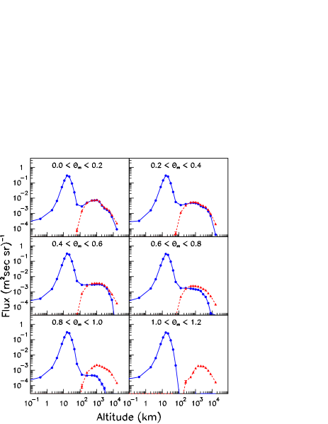
Figure 9: Integrated antiproton flux versus detection altitude in bins of latitudes between equator and poles, for downward (solid line) and upward (dashed line) $\overline{p}\;$flux.

IV.7 Flux dependence on the altitude

The $\overline{p}\;$flux has been calculated up to altitudes of 2 10⁴ km with the aim of investigating the general features of the dynamics and kinematics of the particles in the more remote Earth environment than considered in the previous sections.

Figure 9 shows the altitude dependence of the energy integrated upward and downward $\overline{p}\;$flux in bins of latitude, assuming a geometrical acceptance of 30^∘ for the detector. The calculated distributions display two main features:
1) In the atmospheric range of altitudes, a large peak of incoming flux centered around 20 km and corresponding to atmospheric secondaries, dominates the distribution ($\lesssim$ 50km, i.e., $\lesssim$TOA), with basically no associated outgoing flux (inside the quoted acceptance angle).
2) Above the atmosphere, surprisingly, the calculated upward and downward flux are found close to each other up to fairly high altitudes, namely $\approx$10⁴ km, for the low and intermediate latitudes ($|\theta_{M}|\lesssim 0.7$ rad). This shows that a population of quasi-trapped, particles should be observed in this region of space, i.e., up to around five to ten thousands kilometers. This is confirmed by the lifetime of the particle between their production and their absorption, and by the number of bounces of the particles between the mirror points of their trajectories, which extend up to 100 seconds and several 10² bounces (see Fig. 3), respectively for the simulation sample produced. At higher latitudes with ($|\theta_{M}|\gtrsim 0.7$ rad), the incoming flux progressively disappears, and the outgoing flux then corresponds to escape particles.

From these calculations it can be concluded that there should exist a significant flux of quasi-trapped particles extending approximately over a decade of altitudes, from about 50 km (TOA) up to $\approx$10⁴ km, depending on the particle energy and latitude. This flux has been observed already by the AMS experiment in the lower part of the altitude range (380 km) PAP1 . Note that the issue was discussed long ago in a pioneering paper about the electron flux GR77 . See also BA03 (companion paper) for a complementary discussion. The energy spectrum of this flux extends up to around 10 GeV, which is about the upper momentum limit (8.5  GeV) for which particles can match the simple geometrical condition that the gyration radius is smaller than the mean trajectory radius to the upper atmosphere (for equatorial latitude trajectories, at the limit of large, close to $\pi$/2, pitch angles).

Future embarked experiments should take these features into account, even though, in principle, the accurate knowledge of the kinematical conditions of the particle at the detection point allows to know whether it is or not of atmospheric origin.

V Summary and conclusion

In summary, the secondary antiproton flux produced by the Cosmic Ray proton and Helium flux on the atmosphere has been calculated by Monte-Carlo simulation. The flux calculated for the altitude of 2770 m is in fair agreement with the recent BESS measurements. At sea level, it is small but measurable and could provide a natural facility for testing the identification capability of existing experiments or of future devices. For balloon altitudes, the calculated flux has been found in agreement with the values calculated in previous works. At satellite altitudes (380 km) it appears to be negligible compared to the CR flux for polar latitudes, and of the same order of magnitude as for the high balloon altitudes for equatorial and intermediate latitudes (below the geomagnetic cutoff), indicating that it will have to be taken into account in future measurements of the galactic antiproton flux at similar altitudes.

Acknowledgements: The authors are indebted to V. Mikhailov for helpful discussions on the issue and for pointing ref GR77 to them. They are also grateful to M. Nozaki, M. Fujikawa, and the BESS collaboration, for providing their measurements of $\overline{p}\;$flux at 2770 m prior to publication.

References

- (1) F. Donato et al., Ap.J. 563(2001)172
- (2) F.W. Stecker and S. Rudaz, ApJ. 325(1988)16
- (3) A. Bottino et al., Phys. Rev. D58(1999)123503
- (4) L. Bergström, J. Edsjo, and P. Ullio, Proc 26th ICRC, Salt-Lake city, Aug 17-25, 1999; astro-ph/9902012
- (5) B. Carr, ApJ. 206(1976)8
- (6) A. Barrau, Astro. Part. Phys. 12(2000)169 and references included.
- (7) T.K. Gaisser and R.K. Schaefer, ApJ 394(1992)174
- (8) P. Chardonnet, G. Mignola, P. Salati, and R. Taillet, Phys. Lett. B384(1996)161
- (9) M. Simon, A. Molnar, and S. Roesler, ApJ 499(1998)250
- (10) J.W. Bieber et al., Phys. Rev. Lett. 83(1999)675
- (11) P. Ullio, astro-ph/9904086
- (12) I.V. Moskalenko, A.W. Strong, and M.S. Potgieter, ApJ 565(2002)280
- (13) M. Boezio et al., ApJ 561(2001)787
- (14) S. Orito et al., Phys. Rev. Lett. 84(2000)1078
- (15) S.T. Maeno et al., Astro Part Phys 16(2001)121
- (16) M. Boezio et al., ApJ 487(1997)415
- (17) Ch. Pfeifer, S. Roesler, and M. Simon, Phys. Rev. C54(1996)882
- (18) T.K. Gaisser et al., 26th ICRC, Salt-Lake City, 17-25 Aug. 1999, vol 3, p 69.
- (19) D. Maurin, PhD thesis, Université de Savoie, Chambéry, France, Feb. 2001.
- (20) A.E. Hedin, J. Geophys. Res 96(1991)1159
- (21) J.J. Engelmann et al. A&A 233(1990)96 W.R. Webber et al., ApJ 457(1996)435 W.R. Webber et al., ApJ 508(1998)940
- (22) B. Baret, L.Derome, C.Y.Huang, and M. Buénerd, Phys. Rev. D, *** companion paper ***
- (23) L. Derome et al., Phys. Lett. B489(2000)1
- (24) L. Derome, Y. Liu, and Buénerd M., Phys. Lett. B515(2001)1
- (25) L. Derome and M. Buénerd, Phys. Lett. B521(2001)139
- (26) Yong Liu, L. Derome and M. Buénerd, Phys. Rev. D67,073022(2003)
- (27) The AMS collaboration, J. Alcaraz et al., Phys. Lett. B472(2000)215; ibid, Phys. Lett. B490(2000)27
- (28) The AMS collaboration, J. Alcaraz et al., Phys. Lett. B494(2000)19
- (29) M. Boezio et al., ApJ 518(1999)457
- (30) W. Menn et al., ApJ 533(2000)281
- (31) T. Sanuki et al., ApJ 545(2000)1135
- (32) J.S. Perko, Astro. Astrophys. 184(1984)119; see M.S. Potgieter, Proc. ICRC Calgary, 1993, p213, for a recent review of the subject.
- (33) K. Goulianos, Phys. Rep. 1001(1983)169
- (34) Y.D. Bayukov et al., Sov. J. of Nucl. Phys. 42(1985)116
- (35) T. Abbott et al. Phys. Rev. D 45(1992)3906
- (36) A. Boudard, J. Cugnon, S. Leray and C.Volant, submitted to Phys. Rev. C
- (37) Y. Sugaya et al., Nucl. Phys. A634(1998)115;
- (38) T. Abbott et al., Phys. Rev. C 47(1993)1351;
- (39) J. V. Allaby et al., Report CERN/70-12 (1970);
- (40) T. Eichten et al., Nucl. Phys. 44(1972)333
- (41) A.N. Kalinovski, M.V. Mokhov, and Yu.P. Nikitin, Passage of high energy particles through matter, AIP ed., 1989, Chap. 3
- (42) C.Y. Huang and M. Buénerd, report ISN 01-018, March 2001, to be published.
- (43) C.Y. Huang, PhD thesis, Université J.Fourier, Grenoble (France), May 2002.
- (44) R. Duperray, C.Y. Huang, K. Protasov, and M. Buénerd, astro-ph/0305274, May 15, 2003. submitted to Phys. Rev. D
- (45) Jaros J. et al., Phys. Rev. C18(1978)2273
- (46) D. Armutliiski et al. Sov. J. of Nucl. Phys. 45(1987)649
- (47) S. Baskovic et al., Phys. At. Nucl. 56(1993)540
- (48) A. Bialas, M.Bleszynski, and C.W.Czyz, Nucl. Phys. B111(1976)461
- (49) M.A. Faessler Phys. Rep. 115(1984)1
- (50) J.R. Letaw, R. Silberberg, C.H. and Tsao, Ap.J. Suppl, 51(1983)271
- (51) A.S. Carroll et al, Phys. Lett. B 80(1979)319; C. Denisov et al., Nucl. Phys. B61(1973)62; K. Nakamura et al., Phys. Rev. Lett. 52(1984)731; C. Barbina et al., Nucl. Phys. A612(1997)346.
- (52) A. Baldini et al., Landolt-Börnstein New Series, Vol I/12b, Springer Verlag, 1988
- (53) C.Y. Huang et al., 27th ICRC, Hamburg, Aug. 9-15, 2001
- (54) S.F. Singer and A.M. Lenchek, Prog. in Elem. Part. and Cosm. Ray Phys., Vol 6, p 245, NHPC, 1962.
- (55) C. Störmer, The Polar Aurora, Clarendon Press, Oxford, 1955
- (56) R. Gall and J. Lifschitz, Proc. IUPAP Cosmic Ray Conf., Moscow 1960, Ed. S.I. Syrovatsky, Vol 3, p 64.
- (57) N.L. Grigorov, Sov. Phys. Dokl. 22(1977)305
- (58) M. Buénerd, Int. J. Mod. Phys. 17(2002)1665
- (59) M. Fujikawa, Thesis, University of Tokyo, 2001.
- (60) S.A. Stephens, Astropart. Phys. 6(1997)229
- (61) Y. Ajima et al., Nucl. Inst. and Meth. in Phys., A443(2000)71; Y. Asao et al., Nucl. Inst. and Meth. in Phys., A416(1998)236
- (62) The AMS collaboration, J. Alcaraz et al., Phys Rep 336(2002)331
- (63) I.V. Moskalenko, A.W. Strong, S.G. Mashnik, J.F. Ormes., astro-ph/0210480, Oct 2002; ibid, astro-ph/0301450, LANL-REPORT-LA-UR-02-7813, Jan 2003.
- (64) A. Menchaca-Rocha, private communication.
- (65) See http://www.auger.unam.mx/cln/