Extending emission line Doppler Tomography ; mapping modulated line flux

Abstract

Emission line Doppler tomography is a powerful tool that resolves the accretion flow in binaries on micro-arcsecond scales using time-resolved spectroscopy. I present an extension to Doppler tomography that relaxes one of its fundamental axioms and permits the mapping of time-dependent emission sources. Significant variability on the orbital period is a common characteristic of the emission sources that are observed in the accretion flows of cataclysmic variables and X-ray binaries. Modulation Doppler tomography maps sources varying harmonically as a function of the orbital period through the simultaneous reconstruction of three Doppler tomograms. One image describes the average flux distribution like in standard tomography, while the two additional images describe the variable component in terms of its sine and cosine amplitudes. I describe the implementation of such an extension in the form of the maximum entropy based fitting code MODMAP. Test reconstructions of synthetic data illustrate that the technique is robust and well constrained. Artifact free reconstructions of complex emission distributions can be achieved under a wide range of signal to noise levels. An application of the technique is illustrated by mapping the orbital modulations of the asymmetric accretion disc emission in the dwarf nova IP Pegasi.

1 Introduction

The presence of prominent emission lines in the spectra of close binaries is one of the tell-tale signs of an accretion flow. The highly structured and time dependent emission line profiles observed in cataclysmic variables (CVs) and X-ray binaries harbour a wealth of information. Since the flow is highly supersonic, the overall line profile shape is not determined by the local line profile. Instead, it is dominated by the dynamics of the flow, thus providing a direct kinematical signature of the accretion structure (Smak 1981, Horne & Marsh 1986). This motivated the development of Doppler tomography (Marsh & Horne 1988) as a tool to recover the accretion flow from the observed line profiles in CVs. It was recognised that the observed line profile at each orbital phase is a projection of the accretion flow along the line of sight, and given sufficient observed projection angles, the profiles can be inverted to give the line emission distribution in the binary. Such different projection angles are naturally provided to us as the binary components orbit their common centre of mass as a function of the orbital period permitting reconstructions that resolve the accretion flow on micro-arcsecond scales. I refer to Marsh (2002) and Horne (1991) for the basic details concerning the inversion process from data to Doppler maps, a process which shares many similarities with medical CAT-scanning procedures. Since one observes the radial velocities of the emitting material in the line profiles through Doppler shifts, the choice of working in velocity space is one of the major advantages of standard Doppler tomography. While not perhaps as intuitive to interpret as spatial images in the Cartesian X-Y frame, Doppler tomograms in $V_{x}-V_{y}$ velocity space can be obtained without specific prior assumptions concerning the velocity field in the flow as a function of position. This significantly simplifies the inversion process and allows the application of Doppler tomography in a variety of conditions where the nature of the flow is not a-priori known. Since its conception, Doppler tomography has grown to become a widely used tool with over 100 papers in the refereed press presenting Doppler images. For recent reviews and a number of examples of its application see Boffin, Steeghs & Cuypers (2002). Despite its flexibility, Doppler tomography rests on certain assumptions and approximations. In this paper, I present an extension to Doppler tomography that relaxes one of its main assumptions, thus further increasing its applicability. I will start by reviewing the basic axioms of tomography in Section 2, the implementation of the extension is described in Sections 3 and 4, and the new code is scrutinised in Sections 5 and 6.

2 The axioms of Doppler tomography

Standard tomography reconstructs the distribution of line emission in the binary in a velocity coordinate frame. It effectively decomposes the observed line profiles into discrete emission sources characterised by their velocity vector in the co-rotating frame of the binary. I start by reviewing the basic axioms of Doppler tomography as given in Marsh (2002), albeit in a different order;

1. the intrinsic line profile width is negligible

2. all velocity vectors co-rotate in the binary

3. motion is mapped parallel to the orbital plane only

4. all points are equally visible at all times

5. the flux from any point is constant in time

Violations of these assumptions do not imply that Doppler tomography cannot be performed, or that the maps are meaningless, but these assumptions must be borne in mind when interpreting Doppler maps. As such, the tomogram is a representation of the observed data given the above assumptions and the accuracy and reliability of that representation is thus intimately tied in with the validity of the above axioms.

For example, the local line profile is expected to be set by a thermally broadened profile, amounting to a width of order 10 km/s for typical CV temperatures. Compared to Doppler velocities of hundreds to thousands of km/s makes axiom 1 generally satisfied under a wide range of conditions. However, non-thermal broadening mechanisms may be at work in parts of the flow, and can in particular affect low velocity emission. Axioms 2 and 3 can be violated in parts of the flow, but the derived Doppler map should then be seen as approximations whereby the flow is projected onto the orbital frame of the binary and the map provides a time averaged representation of the flow in the co-rotating frame. Of the five axioms, number four is the most difficult to deal with since one does not generally know the full geometry of the flow that is being mapped. After all, the whole point of Doppler mapping is to probe this geometry. In high inclination systems, self-shadowing effects may play a role, and complicate the analysis of emission line profiles.

This leads us to the remaining axiom, that is the flux from each point in the co-rotating frame is assumed constant in time. However, observations show that the typical emission sources one is mapping do modulate their flux in time. This can be because the line source emits an-isotropically (e.g. the emission from density waves and shocks in an accretion disc) or because axiom 4 is violated and the geometry is responsible for a strong modulation of the flux (e.g. the buried bright spot or the irradiated secondary star) or a combination of both. Doppler tomography can still be used in that case, since the Doppler map serves to present a time averaged image of the distribution of line emission, ignoring such phase-dependent complications. However, one will not be able to fit the data very well, and the phase dependent information contained in the observed line profiles is lost. This motivated the development of an extension to Doppler tomography that allows the line flux from a given point to vary as a function of time. The next Sections concern the implementation of such an extension which I refer to as modulation Doppler tomography.

3 Mapping modulated emission

In conventional Doppler tomography, each line source is characterised by its inertial velocity vector ${\bf V}=(V_{x},V_{y})$, where the binary centre of mass is at the origin, the x-axis points from the accretor to the donor and the y-axis point in the direction of motion of the donor, as viewed in the co-rotating frame of the binary. The intensity of the Doppler map at a given velocity $I(V_{x},V_{y})$ describes the line flux observed from the velocity element with centre $(V_{x},V_{y})$ and width $(dV_{x},dV_{y})$. Each velocity vector follows a sinusoidal radial velocity curve $V(\phi)$ in the inertial frame of the observer as a function of the orbital phase $\phi$ given by:

$$V(\phi)=\gamma-V_{x}\cos{2\pi\phi}+V_{y}\sin{2\pi\phi}$$ (1)

where $\gamma$ is the systemic velocity of the binary system and phase zero is defined to be inferior conjunction of the donor star with $0<\phi<1$. Each line source contributes a constant amount to the observed line profiles at each phase (axioms 4 and 5), and the observed line profile $F(v_{r},\phi)$ is simply a projection of the radial velocities and intensities of all velocity vectors considered;

$$F(v_{r},\phi)=\int I(V_{x},V_{y})\star g(V-v_{r})\mbox{ }dV_{x}dV_{y}$$ (2)

with $g(V-v_{r})$ describing the local line profile intensity at a Doppler shift of $V-v_{r}$, which is usually assumed to be a Gaussian profile with a width corresponding to the instrumental resolution. Let us now consider line sources that modulate harmonically in flux as a function of the orbital phase;

$$f(\phi)=I_{avg}+I_{cos}\cos{2\pi\phi}+I_{sin}\sin{2\pi\phi}$$ (3)

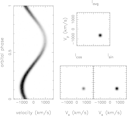
Figure 1: The signature of a time dependent emission source is not only characterised by its radial velocity curve $V(\phi)$, but also its emission strength along its velocity trajectory as a function of time; $f(\phi)$. $V(\phi)$ is characterised by its coordinate $(V_{x},V_{y})$ in the Doppler coordinate frame (Eqn. 1) whereas $f(\phi)$ is characterised by the amplitudes $I_{avg}$, $I_{cos}$ and $I_{sin}$ (Eqn. 3). All modulations on the orbital period can then be described as the sum of the image values in the three Doppler images.

One then has three parameters to describe the line flux from a specific velocity vector; the average line flux $I_{avg}$ and the amplitude and phase of the modulation in terms of $I_{cos}$ and $I_{sin}$. This in contrast to the single parameter $I(V_{x},V_{y})$ in Doppler tomography as described above. In this prescription, we need three Doppler maps describing the values of $I_{avg}$,$I_{cos}$ and $I_{sin}$ for each velocity $(V_{x},V_{y})$ (see Figure 1). The total amplitude of the modulation is then $\sqrt{I_{cos}^{2}+I_{sin}^{2}}$, and its phase is $\tan^{-1}(I_{cos}/I_{sin})$. In terms of Equation 2, this amounts to replacing $I(V_{x},V_{y})$ with $I_{avg}(V_{x},V_{y})+I_{cos}(V_{x},V_{y})\cos(2\pi\phi)+I_{sin}(V_{x},V_{y})\sin(2\pi\phi)$. This extension is thus straightforward to implement, and does not fundamentally alter the nature of the projection from data to maps and vice-versa. Rather then constructing one Doppler map, one now has three Doppler maps characterising the nature of the emission across the co-rotating frame. While I could have allowed for a more complicated type of modulation, either by including more terms to account for non-sinusoidal modulations, or by letting the period of modulation to be different from the orbital period, the above implementation provides a simple and flexible prescription with minimal additional free parameters to fit the observed data with.

4 Implementation of MODMAP

The inversion process from observed data to Doppler maps is normally done via either the back-projection method in combination with Fourier filtering (Horne 1991) or maximum entropy regularisation (Marsh & Horne 1988). For a comparison of the relative merits of both methods in the light of Doppler tomography see Marsh (2002). For the implementation of the modulation Doppler tomography code, I choose to employ the maximum entropy route, since a back-projection would suffer from serious cross-talk between the three image terms and produce significant imaging artifacts. The Fortran code MODMAP uses the MEMSYS algorithm (Skilling & Bryan 1984) in order to iteratively adjust the Doppler images while achieving a user specified $\chi^{2}$. The algorithm gradually steers toward the requested $\chi^{2}$ value while maximising the entropy of the images in order to converge to a unique solution. It delivers the simplest image that can fit to data to the specified level, whereby simplicity is reflected by the image entropy (see also Horne 1994). This image entropy ($S$) of an image vector ${\bf I}=I(1,..N)$ is defined relative to a template image of the same dimension, the default map ${\bf D}$:

$$S=\sum^{N}_{i=1}(D(i)-I(i))+I(i)ln(I(i)/D(i))$$

Using such a maximum entropy regularised fitting scheme, the final solution is determined by the requested $\chi^{2}$ value and the choice of default. The entropy is maximised (approaches zero) as ${\bf I}$ approaches ${\bf D}$. Since the entropy is only defined for positive image values, but the cosine and sine amplitudes of the modulation can be both positive or negative, the Doppler image vector passed to the fitting code was split into a sequence of five velocity maps. The first image array represents the average image values ($I_{1}=I_{avg}$), while the cosine and sine values are represented by two image arrays each. For those two images, one image reflects positive amplitudes, the other negative amplitudes such that $I_{cos}=I_{2}-I_{3}$ and $I_{sin}=I_{4}-I_{5}$. In this way all possible modulations are included while a positive image vector is maintained under all circumstances for which an entropy can be defined.

For the default image vector, I experimented with several options, and the commonly used running default method using a blurred version of the image vector was implemented because of its good convergence properties. In this scheme, the default is recalculated after each iteration by heavily blurring the current image in velocity space, providing a smooth default that only contains large scale image structure. In order to minimise structure in the modulation images $I_{2}-I_{5}$, the defaults for these were steered to zero after blurring. The velocity grid ($N_{x}\times N_{y}$) of the Doppler images is user defined, finer grids requiring significantly more CPU time for each iteration since the number of pixels in the image vector is $5\times N_{x}\times N_{y}$. In order to speed up the iterative fitting procedure, an optimal value was sought for the initial average image ($I_{1}$) through $\chi^{2}$ minimisation of a constant scaling factor. The other four images were started off at zero. The MODMAP code would then iterate to a user specified $\chi^{2}$ until converged at the maximum entropy solution.

5 Test reconstructions

In order to test the reliability of the modulation Doppler tomography technique, and to explore image artifacts due to both random and systematic errors, a large set of test data sets were generated. Time-dependent line profiles were synthesised and passed to the MODMAP code so that its reconstructions could be compared with the original input data. In this Section, I discuss a selection of these reconstructions. They will illustrate the robustness of the image reconstructions, and explore the possible effects of external systematic errors.

5.1 Reconstruction 1: Independent spots

The first test data set concerns the reconstruction of three isolated emission spots, each at a different inertial velocity and with different modulation characteristics. The first spot does not modulate at all, has a FWHM of 100 km/s and unit strength. The second spot is broader (250 km/s) and modulates strictly in a cosine fashion with 90% amplitude, while the third spot modulates strictly in sine fashion with an amplitude of 50%. The corresponding Doppler maps for these spots are presented in Figure 2, and test data was generated from these maps. After adding random Poisson-type noise, the simulated data was loaded into the MODMAP code in order to reconstruct the Doppler maps. As Figure 2 illustrates, the code reconstructs these spots perfectly, in terms of their velocity location, overall strength and width as well as modulation amplitudes. Most importantly, no cross talk is present between the modulation images in the sense that there is no remnant of a pure cosine source in the sine image and vice versa.

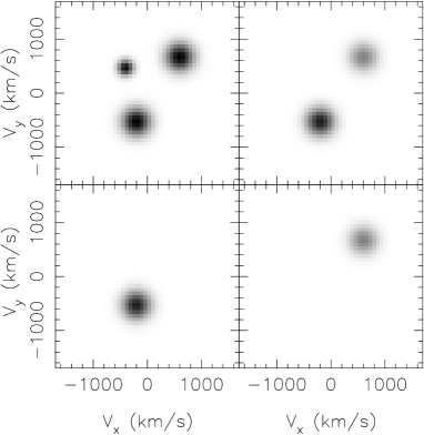
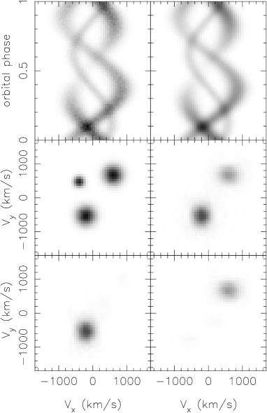
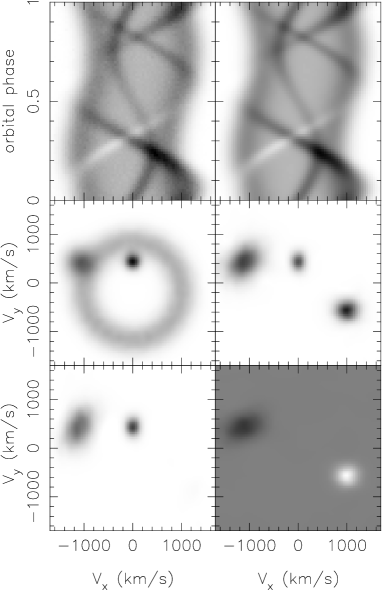
Figure 2: Examples of test reconstructions based on synthetic data sets. Top panels indicate the input Doppler maps, expected to be recovered given perfect signal to noise and data sampling. The four maps in each panel correspond to, starting top-left and moving in clockwise fashion; the average emission, the total modulated emission, the sine amplitude map and the cosine amplitude map. Below the cosine input maps are the generated line profiles, after Poisson noise was added. The recovered Doppler images are plotted in the bottom panels, and the predicted line profiles based on these maps, used to evaluate the goodness of fit, are presented to the right of the input line profiles. The grayscale is chosen such that black corresponds to the maximum value of the images, and white to the lowest. In case of negative image values, zero corresponds to 50% gray.

5.2 Reconstruction 2: Disc plus spots

For the second reconstruction, I chose a more complex and demanding emission pattern reminiscent of the common emission sources found in CVs. The first component was a non-varying accretion disc contribution centred at slightly negative $V_{y}$ velocities (the velocity of the accretor), represented by a ring in the Doppler coordinates. Then a narrow spot was added at the typical location of the mass donor star ($V_{x}=0$,$V_{y}=400$ km/s). This spot modulates in a purely cosine fashion with 50% amplitude and it is just separated from the disc emission in terms of its velocity. A second spot representative of a disc hot-spot was added with a contribution to all three Doppler images (40% modulation amplitude in both the sine and cosine terms). Its velocities overlap with that of the disc emission. Finally, a third spot was included, again overlapping with the disc emission in terms of velocity, and this time with a pure sine modulation with a negative amplitude of 50%. I refer to Figure 2 for the corresponding input images and data, and the results from the MODMAP reconstruction. The code again recovers the original image structure very well. The modulation amplitudes are reproduced correctly, and the spots are cleanly separated from the disc emission. Thus even sources that overlap in velocity but have different modulation characteristics are reproduced correctly and without artifacts or cross talk. This holds true even at low signal to noise levels. In Figure 3a we illustrate the same reconstruction, after degrading the signal to noise of the input data to only 5. As expected, the image structure recovered is a blurred version of the original, due to the low signal to noise of the data. However, the spot properties are still reproduced correctly and without cross-talk. Provided that the modulation is of sufficient amplitude to be significant given the signal to noise of the data, the reconstructions are stable for a wide range of signal to noise levels. In such cases where low signal is a concern, the significance of reconstructed features can be assessed using Monte-Carlo methods (Marsh 2002). An ensemble of reconstructions should be made using bootstrapped copies of the input data, in order to quantify the pixel-dependent variance in the Doppler tomograms.

These two test reconstruction served to illustrate the robustness of the reconstruction method, and to confirm that artifact free reconstructions can be reconstructed from complex time-dependent emission sources. When reconstructing Doppler maps from real data, two parameters need to be established; the systemic velocity $\gamma$, and the local line profile function $g(v)$. The next two reconstructions illustrate the artifacts that can be introduced by a significant error in the estimates for these parameters.

5.3 Reconstruction 3: Incorrect systemic velocity

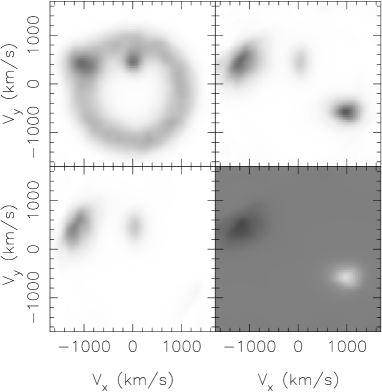
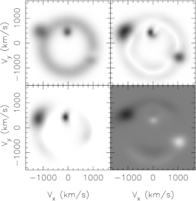
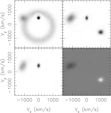
Figure 3: Test reconstructions of synthetic data based on the same input maps as presented in Figure 2b. Top left (a) is reconstruction after degrading the signal to noise of the data to 5. Top right (b) is the reconstruction achieved while assuming an incorrect systemic velocity. The bottom plots illustrate the result after underestimating the local line profile width by a factor of two (c; left), and overestimating it by the same factor (d; right).

The systemic velocity needs to be known in order to calculate the correct radial velocity curve (Eqn 1) of a line source with velocity ($V_{x}$,$V_{y}$). If one attempts to reconstruct a data set with an incorrect gamma, it will be difficult to achieve a good fit to the data since the code is not tracing the correct velocity curves (see also Marsh & Horne 1988). Figure 3b illustrates the reconstructed Doppler images using the same data set that was employed in the previous test reconstruction, but now reconstructing it with a systemic velocity that is incorrect by 60 km/s. Clear artifacts are present in all the maps, and the code, as expected, is unable to achieve a reduced $\chi^{2}\sim 1$. Thus, an incorrectly assumed gamma can lead to significant artifacts in the modulation maps, more so than in the average map. The total modulation flux map illustrates that the (non-varying) disc in particular leaves artifacts in the modulation images.

For many systems, an estimate of the systemic velocity is known or can be measured from the line profiles. The uncertainty in $\gamma$ only becomes an issue if its error approaches or exceeds the local line profile width. In those cases where the data resolution is very high, or independent $\gamma$ estimates are not available, the achieved $\chi^{2}$ value can be employed as a self-consistent test of the assumed systemic velocity. Since an incorrect $\gamma$ leads to image artifacts and poor data fits, one can perform a series of Doppler map reconstructions while trying to minimise $\chi^{2}$ as a function of $\gamma$ in order to identify the correct systemic velocity. Thus, provided the potential effects of an incorrect gamma are borne in mind, its impact on the image reconstructions can usually be verified self-consistently, and can be used to determine the systemic velocity.

5.4 Reconstruction 4: Error introduced by incorrect local line profile

The local line profile is assumed to be a Gaussian with its width adjusted to the instrumental resolution of the data. In Figure 3c, I illustrate the reconstructed Doppler maps after underestimating the local line width by a factor of two. While the maps show weak fine structure due to this oversampling effect, it still recovers the correct image structure. On the other hand, overestimating the local line width by the same factor leads to a sharpening of the recovered maps (Figure 3d); the reconstructed spot sizes are now too small in the Doppler images and the convergence is very slow. This is the result of the code attempting to reproduce the observed width of the spots with an assumed local line profile that is too broad. This can only be achieved by making the spot widths smaller in the maps. The effect of a forced error in $g(v)$ affects all the maps in the same way, and does not degrade the ability to recover modulated emission sources. It is clearly better to caution on the side of oversampling by underestimating the local line width to avoid artificial sharpening of the tomograms. Thus provided the structures that one is imaging are sampled properly, reconstructions are robust against modest local line width variations.

6 Application to IP Pegasi

As a real world example of the use of modulation mapping, I applied MODMAP to existing data of the eclipsing dwarf nova IP Pegasi during outburst. This data together with conventional Doppler maps were presented in Harlaftis et al. (1999) and revealed strong spiral arms in the accretion disc. Figure 4 plots the reconstructed modulation Doppler maps for the HeII 4686Å emission of IP Pegasi. A much better reconstruction of the observed data was achieved using the MODMAP code compared to the conventional Doppler reconstruction, indicative of significant orbital variability. The average map corresponds in detail to the maps presented in Harlaftis et al. (1999), with a disc dominated by two spiral arms and weak secondary star emission. Most of the modulated flux is dominated by the sine term, with modulation amplitudes of up to 20%. Again, the variable disc emission is concentrated in two arms. However, these arms do not correspond to the location of the spirals in detail, but only overlap partially. Instead, the modulated disc flux is at slightly larger velocities (i.e. closer in) and rotated anti-clockwise in terms of phase. It thus appears that most of the modulation is not due to anisotropic radiation from the spiral arms directly, but variable emission from the disc regions just inside. This could be due to geometric shielding of those disc areas by the vertically extended spiral structures. The phasing of the modulation supports such an interpretation; the emission from the disc just inside the closest arm is weaker compared to that of the disc inside the opposite arm and both modulate in anti-phase. This is expected if the spiral arms are vertically extended, shielding the disc area immediately behind them from the observer at high inclinations (IP Pegasi is an eclipsing system after all). As always, one must bear in mind that although the modulation mapping code is able to show that disc flux is modulated, significant geometrical shielding violates the basic assumptions of Doppler tomography (axiom 4).

As well as modulated emission from the disc, the maps also show that the secondary star and an extended low velocity region are time dependent emission sites. This reconstruction illustrates the ability of MODMAP to identify emission sites in the binary that modulate as a function of the orbital phase and characterise their modulation in terms of its phase and amplitude. It achieves better fits to the data, and aids in establishing the nature of the line emitting sources. A more extensive and quantitative analysis of reconstructions using MODMAP on existing data sets will be presented in future papers.

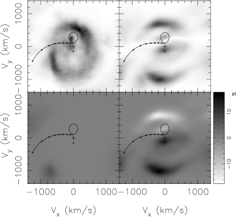
Figure 4: MODMAP reconstructions of the HeII emission from IP Pegasi during outburst (data from Harlaftis et al. 1999). The emission from the asymmetric accretion disc carrying a two armed spiral modulates significantly. The grayscale wedge denotes the fractional modulation amplitudes in the sine and cosine images.

7 conclusions

I presented an extension to emission line Doppler tomography that permits the mapping of time dependent emission sources. It relaxes one of the five fundamental axioms of conventional Doppler tomography, and maps harmonically varying modulations on the orbital period. Since significant variability on the orbital period is a common characteristic of the typical emission sources in CVs and X-ray binaries, this prescription permits a more detailed reconstruction of the nature of the accretion flow. Intrinsic variability not correlated with the orbit is however not described by this extension. Instead of a single Doppler map describing the time averaged emission distribution in the co-rotating frame of the target, modulation Doppler tomography describes the emission through three Doppler tomograms. One describes the average flux distribution just like in standard Doppler tomography, while the two additional tomograms describe the variable component in terms of its sine and cosine amplitudes. Thus for each location in the $V_{x}-V_{y}$ Doppler coordinate frame, the mean flux and the amplitude and phase of any variable flux contribution is given by the three image values at that velocity.

Test reconstructions using the maximum entropy based fitting code MODMAP in conjunction with synthetic data show that the technique is robust, and artifact free reconstructions of complex emission distributions can be achieved under a wide range of signal to noise levels. The effects of systematic uncertainties in the assumed systemic velocity and local line profile width are similar to those seen in conventional tomography.

There are several reasons to expect anisotropic emission from the accretion flow. Horne (1995) explores the signature of anisotropic turbulence on the emission pattern of a turbulent accretion disc. Anisotropy in the turbulence Mach matrix also leads to anisotropic line emission from the disc. The prominent spiral structures seen in dwarf nova accretion discs are also likely to emit an-isotropically (e.g. Steeghs & Stehle 1999) as was illustrated in Section 6. The highly variable emission from the disk-stream impact region (e.g. Spruit & Rutten 1998) is another prime example of orbitally modulated emission. In Morales-Rueda et al. (2003), the results from modeling the bright spot emission in GP Com using MODMAP are presented. Finally, the irradiated secondary star is a common emission line source present in the line profiles (e.g. Marsh & Horne 1990). While the emission from the Roche-lobe shaped donor is better mapped with Roche-tomography techniques (Watson & Dhillon 2002), modulation Doppler tomography is able to reproduce the basic properties of the emission. This permits much better fits to the data, making a strong secondary star contribution less problematic for disc mapping experiments (Steeghs 2002).

Modulation Doppler tomography is a robust and well constrained extension that may assist the interpretation of both existing and future data sets of accreting binaries. As with all tomographic imaging techniques, it nevertheless still relies on several assumptions that need to be borne in mind when interpreting any image reconstructions (Section 2). Its main advantage over conventional Doppler tomography is to describe emission sources that vary harmonically as a function of the orbital phase. Its added flexibility should find a wide range of uses, in particular in conjunction with high signal to noise data.

References

- [BSC] Boffin, H.M.J., Steeghs, D., Cuypers, J., 2002, Eds., Astrotomography ; indirect imaging methods in observational astronomy, Lecture Notes in physics Series Volume 573, Springer Verlag, Berlin
- [h99] Harlaftis, E.T., Steeghs, D., Horne, K., Martin, E., Magazzu A., 1999, MNRAS, 306, 348
- [H91] Horne, K., 1991, in: Fundamental Properties of Cataclysmic Variable Stars, ed. A.W.Shafter, San Diego State Uiversity, San Diego
- [H95] Horne, K., 1995, A&A, 297, 273
- [H94] Horne, K., 1994, in: ASP Conf Series Vol. 69, Gondhalekar, P, Horne, K., Peterson, B., eds., ASP Press
- [HM86] Horne, K., Marsh, T.R., 1986, MNRAS, 218, 761
- [M02] Marsh, T.R, 2002, in: Astro-tomography, Boffin, H., Steeghs, D., Cuypers, J, eds., Lecture Notes in Physics Series 573, Springer Verlag
- [MH90] Marsh, T.R., Horne, K., 1990, ApJ, 349, 593
- [MH88] Marsh, T.R., Horne, K., 1988, MNRAS, 236, 269
- [LMR] Morales-Rueda, L., Marsh, T. R., Steeghs, D., Unda-Sanzana, E., Wood, Janet H., North, R. C., 2003, A&A, in press
- [MEM] Skilling, J., Bryan, R.K., 1984, MNRAS, 211, 111
- [SM81] Smak, J., 1981, AcA, 31, 395
- [SR] Spruit, H., Rutten, R., 1998, MNRAS, 299, 768
- [S02] Steeghs, D., 2002, in: Astro-tomography, Boffin, H., Steeghs, D., Cuypers, J, eds., Lecture Notes in Physics Series 573, Springer Verlag
- [ss99] Steeghs, D., Stehle, R., 1999, MNRAS, 307, 99
- [wd02] Watson, C., Dhillon, V., 2002, MNRAS, 326, 67