Cosmological model with macroscopic spin fluid

Abstract

We consider a Friedmann-Robertson-Walker cosmological model with some exotic perfect fluid with spin known as the Weyssenhoff fluid. The possibility that the dark energy may be described in part by the Weyssenhoff fluid is discussed. The observational constraint coming from supernovae type Ia observations is established. This result indicates that, whereas the cosmological constant is still needed to explain current observations, the model with spin fluid is admissible. For high redshifts $z>1$ the differences between the model with spin fluid and the cold dark matter model with a cosmological constant become detectable observationally for the flat case with $\Omega_{\text{m},0}=0.3$. From the maximum likelihood method we obtain the value of $\Omega_{\text{s},0}=0.004\pm 0.016$. This gives us the limit $\Omega_{\text{s},0}>-0.012$ at the $1\sigma$ level. While the model with “brane effects” is preferred by the supernovae Ia data, the model with spin fluid is statistically admissible. For comparison, the limit on the spin fluid coming from cosmic microwave background anisotropies is also obtained. The uncertainties in the location of a first peak give the interval $-1.4\times 10^{-10}<\Omega_{\text{s},0}<-10^{-10}$. From big bang nucleosynthesis we obtain the strongest limit $\Omega_{\text{s},0}\gtrsim-10^{-20}$. The interconnection between the model considered and brane models is also pointed out.

I Introduction

In 1923 Cartan introduced the intrinsic angular momentum in the theory of relativity (as a classical quantity) Cartan (1923), before it was introduced as spin into quantum theory by Goudsmit and Uhlenbeck in 1925. The classical spin can be introduced in general relativity in two distinct ways. The first one is to introduce spin as a dynamical quantity in special and then in general relativity without changing the geometry, i.e., without modifying the metric of spacetime Mathisson (1937); Honl and Papapetrou (1937, 1939, 1940); Weyssenhoff and Raabe (1947). The spin introduced in this way showed more or less a similarity to the spin of quantum mechanics (and the Dirac theory of the electron). The second, more satisfactory way to introduce the intrinsic angular momentum is by generalizing the structure of spacetime. It was done by Cartan by assuming the metric and the non-symmetric affine connection as independent quantities and was further developed by Hehl Hehl (1974), Trautman Trautman (1972) and Kopczynski Kopczynski (1972, 1973). This assumption allowed a definition of the torsion of spacetime and its connection with the torsion with spin. In the framework of Einstein-Cartan theory for the Friedmann universe Trautman Trautman (1973) made the conclusion that torsion avoids the singularity and stops the collapse in closed models at the moment of minimum radius about 1 cm with matter density $\rho\sim 10^{55}\mathrm{g}\,\mathrm{cm}^{-3}$

$$R_{\mathrm{min}}=\left(\frac{3G\hbar^{2}n}{8mc^{4}}\right)^{1/3},\quad\rho_{\mathrm{max}}=\frac{4m^{2}c^{2}}{3\pi^{2}G\hbar^{2}}.$$

Let us note that the above formulas are valid for chaotic spin distribution Ponomarev et al. (1985). The effects of spin fluid are important in a low-energy limit of the superstring theory (see for general discussion Tassie (1986)) which is supergravity whose integral part is torsion.

The torsion contributes to the energy-momentum of spin fluid which has the form Ivanenko et al. (1985)

$$T_{\mu\nu}^{\mathrm{eff}}=u_{\mu}u_{\nu}(p+\rho-2s^{2})-g_{\mu\nu}(p-s^{2})$$

with $s^{2}=s_{\mu\nu}s^{\mu\nu}$, where the spin $s$ leads to an effective negative pressure and eliminates the singularity.

Let us consider a world model with the Robertson-Walker symmetries which is filled with ‘perfect fluid with spin’. As it is well known Halbwachs (1960) the macroscopic spin tensor $\tau_{\mu\nu}^{\lambda}$ may be expressed in terms of the spin density tensor $S_{\mu\nu}$ and four-velocity of the fluid $u^{\mu}$ ($u_{\mu}u^{\mu}=-1$)

$$\tau_{\mu\nu}^{\lambda}=u^{\lambda}S_{\mu\nu},\qquad S_{\mu\nu}u^{\mu}=0.$$ (1)

To describe the material content of the considered model we use the hydrodynamical description in terms of the energy-momentum tensor which in the general relativity limit reduces to perfect fluid characterized by the energy density $\epsilon$ and the isotropic pressure $p$. In analogy, the physical content of the model in the Einstein-Cartan theory, based on the classical description of spin with equation (1), may be called “perfect fluid with spin”. This is surely the simplest type of hydrodynamic continuum of use for our aims. It is an extension of the well known semi-classical model of spin fluid from special relativity; we call it the Weyssenhoff fluid Weyssenhoff and Raabe (1947). The influence of the macroscopic spin present in the fluid on the dynamics of the universe is then described by contributions to the energy density and pressure

$$\epsilon_{\text{eff}}=\epsilon-\frac{1}{4}S^{2},\qquad p_{\text{eff}}=p-\frac{1}{4}S^{2},$$ (2)

where $S^{2}=\frac{1}{2}S_{\mu\nu}S^{\mu\nu}$ , and $S_{\mu\nu}$ is the spin density tensor Arkuszewski et al. (1974).

Supernovae type Ia observations Garnavich et al. (1998); Perlmutter et al. (1997); Riess et al. (1998); Schmidt et al. (1998); Perlmutter et al. (1998, 1999) indicated that the Universe’s expansion has started to accelerate during recent cosmological times. These observations (as well as cosmic microwave background observations) suggest that the energy density of the Universe is dominated by a dark energy component with negative pressure, driving the acceleration. The most natural candidate to represent dark energy is the cosmological constant. However, it is necessary to require a fine tuning of 120 orders of magnitude in order to obtain agreement with observations Peebles and Ratra (2003).

In this work, we discuss the possibility that some part of the dark energy may be represented by the perfect fluid with spin, which is characterized by an equation of state in form (2).

Let us consider the dust fluid ($p=0$) of particles with spin $1/2$ and mass $m$. The energy density $\epsilon$ and absolute value of the spin density $S$ depend on number $n$ of particles in a unit volume

$$\epsilon=nm,\qquad S=\frac{\hbar}{2}n.$$

Hence we have

$$\epsilon_{\text{eff}}=\epsilon-\left(\frac{\hbar}{4m}\right)^{2}\epsilon^{2},\qquad p_{\text{eff}}=0-\left(\frac{\hbar}{4m}\right)^{2}\epsilon^{2}.$$ (3)

Therefore, effective pressure is negative. Because the number of particles in comoving volume $n(t)\propto a^{-3}(t)$, where $a$ is the scale factor and $\epsilon=\epsilon_{\text{m},0}a^{-3}(t)$ is the energy density of dust, the energy density $\epsilon$ and pressure $p$ are never greater than

$$\epsilon_{\text{max}}=\frac{16m^{2}}{\hbar^{2}},\qquad p_{\text{max}}=-\frac{16m^{2}}{\hbar^{2}},$$

respectively. The energy density of the spin is negative but $\epsilon_{\text{eff}}$ is assumed to be positive. The ratio of the spin-induced term to the standard energy term is

$$\frac{(8\pi GS)^{2}}{8\pi G\rho}=\frac{8\pi G\hbar^{2}\rho}{m^{2}}.$$

With nucleons as dust particles, the above ratio is of the order $8\times 10^{-55}\rho$ (where $\rho$ is expressed in the cgs units). Although the spin-spin contact interaction term appears to be negligibly small even in what may be regarded now as superdense matter, it may play an essential role when the ratio approaches unity, i.e., in the earliest stages of evolution of the Universe. The spin-spin term produces something which may be called after Kopczynski the “centrifugal force” and which is able to prevent the occurrence of singularities in cosmology Kopczynski (1972, 1973).

Let us note now that effects of spin are dynamically equivalent to introducing into the model some additional non-interacting fluid for which the equation of state is

$$p_{\text{s}}=w_{\text{s}}\rho_{\text{s}},$$ (4)

where $w_{\text{s}}=1$, $\rho_{\text{s}}=\rho_{\text{s},0}a^{-6}$, $\rho_{\text{s},0}=-(\hbar^{2}/16)n(0)$, just as for the Zeldovich stiff matter (or brane effects with dust on a brane with negative tension).

II The FRW model with spin on two-dimensional phase plane

The dynamics of the Friedmann-Roberston-Walker (FRW) model with the Weyssenhoff fluid can be represented on the phase plane $(H,\epsilon)$, where $H=d(\ln a)/dt$ is Hubble’s function, in the following way

$$\frac{dH}{dt} =-H^{2}-\frac{1}{6}(\epsilon_{\text{eff}}+3p_{\text{eff}})+\frac{\Lambda}{3}$$ (5a)

$$\frac{d\epsilon}{dt} =-3H\epsilon$$ (5b)

where $p_{\text{eff}}$ and $\epsilon_{\text{eff}}$ are parameterized by the energy density of dust (see formula (3)). Of course, system (5) has the first integral

$$\epsilon_{\text{eff}}-3H^{2}=\frac{3k}{a^{2}}-\Lambda,$$ (6)

where $k\in\{0,\pm 1\}$ is the curvature constant. Additionally, we have the conservation condition for non-interacting spin fluid with energy density $\epsilon$

$$\frac{d\epsilon_{\text{s}}}{dt}=-6H\epsilon_{\text{s}}.$$ (7)

The critical points of (5) can be one of two admissible types: static if $H_{0}=0$, $\epsilon_{0}\neq 0$, or non-static if $H_{0}\neq 0$ and $\epsilon_{0}=0$. In the first case critical points lie on the intersection $H$-axis with the boundary condition $\epsilon_{\text{eff}}+3p_{\text{eff}}=0$ (the cosmological constant is formally included into $p_{\text{eff}}$ and $\rho_{\text{eff}}$ in the standard way $\rho_{\Lambda}=\Lambda$ and $p_{\Lambda}=-\Lambda$). The second type of critical points lie on the intersection of $\epsilon$-axis with the trajectory for flat model $\{\epsilon=3H^{2}\}$.

The physically admissible domain for trajectories is

$$\{(H,\epsilon)\colon H\in\mathbb{R}\quad\text{and}\quad 0\leq\epsilon\leq\epsilon_{\text{max}},\qquad\epsilon_{\text{max}}\colon\epsilon_{\text{eff}}(\epsilon_{\text{max}})=-\Lambda\}.$$

The phase portrait of system (5) with $\Lambda>0$ is demonstrated on Fig. 1.

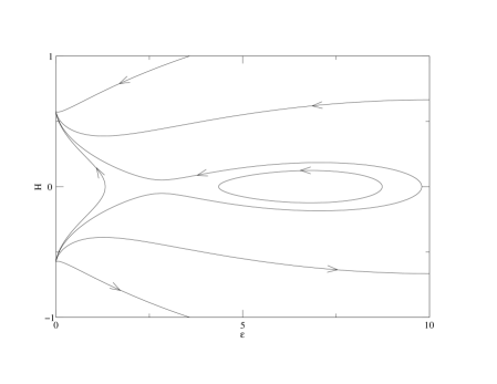
Figure 1: The phase portrait of system (5). There are the four critical points: stable node, unstable node, saddle point and center. The presence of the center in the finite region indicates that the model is structurally unstable.

The differences in the behavior of trajectories are manifest at high densities. Then the structure of dynamical behavior at infinity is modified. To illustrate the behavior of trajectories at infinity, system (5) is represented on Fig. 2 in the projective coordinates

$$z =\frac{1}{H},\qquad u=\frac{\epsilon}{H}, (z,u) -\text{map}$$ (8a)

$$v =\frac{1}{\epsilon},\qquad w=\frac{H}{\epsilon}, (v,w) -\text{map}.$$ (8b)

The two maps $(z,u)\colon z=0,-\infty<u<\infty$ and $(v,w)\colon v=0,-\infty<w<\infty$ cover the behavior of trajectories at the infinity circles $H=\infty$ and $\epsilon=\infty$.

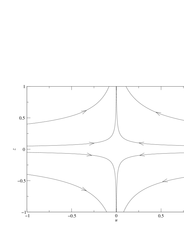
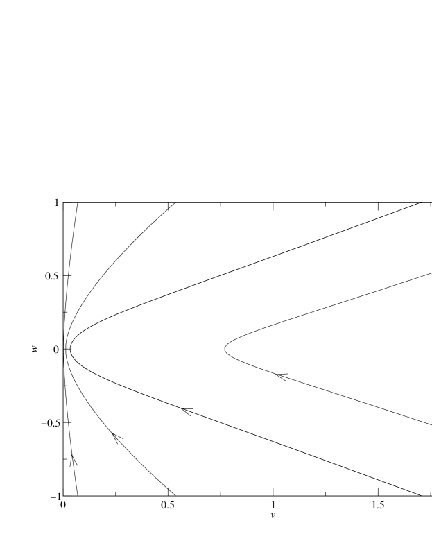
Figure 2: The phase portraits of system (5) in the projective coordinates $(z,u)$ and $(v,w)$. From the portrait in the former coordinates we can see that there is a saddle point in the infinity.

III Dynamics of the model with spin fluid

It is well known that the first integral of the FRW equation can be used to construct a Hamiltonian function. We take advantage of this feature in the considered model. The integration of equation (5b) gives $\rho=\rho_{0}a^{-3}$. Therefore the right-hand side of the Raychaudhuri equation (5a) can be expressed in terms of the scale factor $a(t)$ as

$$\frac{d^{2}a}{dt^{2}}=a\left[-\frac{1}{6}\epsilon_{\text{m},0}a^{-3}+\frac{1}{6}\left(\frac{\hbar}{2}\right)^{2}a^{-6}+\frac{\Lambda}{3}\right].$$ (9)

Equation (9) can be rewritten in a form analogous to the Newton equation of motion in the one-dimensional configuration space $\{a\colon a\in\mathbb{R}_{+}\}$

$$\ddot{a}=-\frac{\partial V(a)}{\partial a}$$ (10)

where the potential function

$$V(a)=-\frac{1}{6}\epsilon_{\text{m},0}a^{-1}+\frac{1}{24}\left(\frac{\hbar}{2}\right)^{2}a^{-4}-\frac{2}{3}\Lambda a^{2}+V_{0}$$ (11)

and $V_{0}=\text{const}$. First integral (6) should correspond with the Hamiltonian integral of motion, hence

$$V(a)+\frac{\dot{a}^{2}}{2}=V_{0}-\frac{k}{2}.$$

Now we construct the Hamiltonian function

$$\mathcal{H}\equiv\frac{\dot{a}^{2}}{2}+V(a)$$ (12)

and then the trajectories of the system lie on the energy level $\mathcal{H}\equiv E$, but if we choose $V_{0}=k/2$ then the physical trajectories lie on the zero-energy level $\mathcal{H}=E=0$, which coincides with the form of first integral (6). Then finally we obtain

$$V(a)=-\frac{1}{6}\epsilon_{\text{m},0}a^{-1}+\frac{\hbar^{2}}{96}n(0)a^{-4}-\frac{1}{6}\Lambda a^{2}+\frac{k}{2}$$ (13)

or in general

$$V(a)=\frac{1}{6}\int^{a}(\epsilon_{\text{eff}}+3p_{\text{eff}})ada=-\frac{1}{6}\epsilon_{\text{eff}}a^{2}-\frac{\Lambda}{2}a+\frac{k}{2}$$ (14)

where

$$\epsilon_{\text{eff}}(a)=\epsilon(a)+\epsilon_{\text{s},0}a^{-6},\qquad\epsilon_{\text{s},0}=-\frac{1}{16}\hbar^{2}n(0),$$

and $n(0)$ is an initial number of particles in the unit comoving volume.

Finally we obtain dynamics reduced to the form of particle like problem in the one-dimensional potential

$$\dot{x} =y$$ (15a)

$$\dot{y} =-\frac{\partial V}{\partial x}$$ (15b)

with

$$V(x)=-\frac{1}{6}(\epsilon_{\text{m},0}x^{-1}+\epsilon_{\text{s},0}x^{-4}-\epsilon_{\Lambda,0}x^{2}-3k)$$ (16)

where $x=a$, $y=\dot{a}$ and the above system has the first integral

$$\frac{y^{2}}{2}+V(x)=0.$$ (17)

In order, basic dynamical system (15) is then rewritten as

$$\frac{\dot{v}^{2}}{2} =\frac{1}{2}\Omega_{k,0}+\frac{1}{2}\sum_{i}\Omega_{i,0}v^{-(1+3w_{i})}$$ (18a)

$$\ddot{v} =-\frac{1}{2}\sum_{i}\Omega_{i,0}(1+3w_{i})v^{-(2+3w_{i})}$$ (18b)

where $v\equiv a/a_{0}$, $t\to T\equiv|H_{0}|t$ is a new time variable denoted as dot in (18); $\Omega_{i}\in\{\Omega_{\text{m},0},\Omega_{\text{s},0},\Omega_{\Lambda,0}\}$ are density parameters, $\Omega_{i}=\rho_{i}/\rho_{\text{cr}}$, $\Omega_{i,0}=\rho_{i,0}/3H_{0}^{2}$ and the subscript $0$ means that a quantity with this subscript is evaluated today (at time $t_{0}$); $\rho_{i}=\rho_{i,0}a^{-(1+w_{i})}$, where $w_{\text{m}}=0$ (dust), $w_{\text{s}}=1$ (spin fluid), $w_{\Lambda}=-1$ (cosmological constant), and $p_{i}=w_{i}\rho_{i}$.

The representation of dynamics as a one-dimensional Hamiltonian flow allows to make the classification of possible evolution paths in the configuration space which is complementary to phase diagrams. It also makes simpler to discuss the physical content of the model. Finally, the construction of the Hamiltonian allows to study quantum cosmology models with spin fluid in full analogy to what is usually done in general relativity.

From equation (14) we can observe that trajectories are integrable in quadratures. Namely, from the Hamiltonian constraint $\mathcal{H}=E=0$ we obtain the integral

$$t-t_{0}=\int_{a_{0}}^{a}\frac{da}{\sqrt{-2V(a)}}.$$ (19)

For some specific forms of potential function (16) we can obtain exact solutions.

It is possible to make the classification of qualitative evolution paths by analyzing the characteristic curve which represents the boundary equation of the domain admissible for motion. For this purpose we consider the equation of zero velocity, $\dot{a}=0$ which constitutes the boundary $\mathcal{M}=\{a\colon V(a)=0\}$.

From equation (16) the cosmological constant can be expressed as a function of $x$ as follows

$$\Lambda(x)=x^{-2}(\epsilon_{\text{m},0}x^{-1}-\epsilon_{\text{s},0}x^{-4}-3k).$$ (20)

The plot of $\Lambda(x)$ for different $k$ is shown in Fig. 3. The domain under the curve $\Lambda(x)$ is non-physical, and we consider the evolution path as a level of $\Lambda=\text{const}$ and we classify all evolution models with respect to their quantitative properties of dynamics. For negative $\Lambda$ there are oscillating solutions without a singularity.

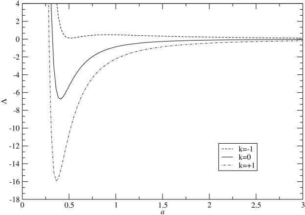
Figure 3: The dependence of $\Lambda$ on $a$.

The next advantage of representing dynamics in terms of Hamiltonian is possibility to discuss how trajectories along which the acceleration condition $\ddot{a}=-dV/da>0$ is satisfied are distributed in the phase space. One can easily observe this phenomenon from the geometry of the potential function. In the phase plane the area of acceleration is determined by $\dot{y}>0$ or by the condition that $V(x)$ is a decreasing function of its parameter

$$-\frac{1}{2}\Omega_{\text{m},0}v^{-2}-2\Omega_{\text{s},0}v^{-5}+\Omega_{\Lambda,0}v>0$$ (21)

where

$$v=\frac{a}{a_{0}},\qquad\Omega_{\text{s},0}\leq 0,\qquad\Omega_{k,0}=0.$$

Independent observations of supernovae type Ia made by the Supernovae Cosmology Project and High-z Survey Team indicate that our Universe is presently accelerating. There is a fundamental problem in explaining this acceleration. If we introduce the cosmological constant and assume $\Omega_{k,0}=0$ (the universe is flat) then the best fit model is $\Omega_{\Lambda,0}=0.72$, $\Omega_{\text{m},0}=0.28$.

The effects of spin fluid cannot dominate the matter contributions during the whole evolution of the universe. But we argue that the effects of spin degree of freedom are important in early universe. In any case they should be smaller than or comparable with the matter contribution because

$$\frac{H^{2}}{H_{0}^{2}}=\Omega_{\mathrm{m,0}}x^{-3(1+\gamma}+\Omega_{\mathrm{s},0}x^{-6}\geq 0.$$

The formalism presented gives us a natural base to discuss this problem for the FRW model with the Weyssenhoff fluid. It is convenient to introduce a new variable $z=v^{-3}$ , then inequality (21) reduces to the quadratic inequality

$$-\frac{1}{2}\Omega_{\text{m},0}z+2|\Omega_{\text{s},0}|z^{2}+\Omega_{\Lambda,0}>0.$$

Therefore the Universe is presently accelerating provided that

$$-\frac{1}{2}\Omega_{\text{m},0}+2|\Omega_{\text{s},0}|+\Omega_{\Lambda,0}>0.$$

For instance, for $\Omega_{\text{m},0}=0.3$, $\Omega_{\Lambda,0}=0$, $|\Omega_{\text{s},0}|>\frac{1}{4}\Omega_{\text{m},0}$ is required. Therefore, present experimental estimates based on baryons in clusters on one hand giving $\Omega_{\text{m},0}\sim 0.3$ and the location of the first peak in the cosmological microwave background detected by Boomerang and Maxima suggesting an early, filled by spin matter, flat universe on the other hand, imply that our Universe without a cosmological term would be presently accelerating only if

$$|\Omega_{\text{s},0}|\gtrsim\frac{1}{3}.$$

The required value of $|\Omega_{\text{s},0}|$ seems to be unrealistic (see the next section) and therefore the cosmological constant term is still needed to explain the present acceleration of the Universe. As we will see in the subsequent analysis the effect of spin fluid is negligible in the present epoch. Therefore the spin is an additional factor that can influence the dynamics of the early universe together with for example the cosmological constant.

IV Redshift-magnitude relation for the model with spin fluid

Cosmic distance measures like the luminosity distance depend sensitively on the spatial geometry (curvature) and the dynamics. Therefore, the luminosity depends on the present density parameters of different components and their form of the equation of state. For this reason the redshift-magnitude relation for distant galaxies is proposed as a potential test for the FRW model with spin fluid.

Let us consider an observer located at $r=0$ at the moment $t=t_{0}$ which receives a light ray emitted at $t=t_{1}$ from the source of the absolute luminosity $L$ located at the radial distance $r_{1}$. The redshift $z$ of the source is related to the scale factor at the two moments of evolution by $1+z=a(t_{0})/a(t_{1})=a_{0}/a$. If the apparent luminosity of the source as measured by the observer is $l$ then the luminosity distance $d_{L}$ of the source is defined by the relation

$$l=\frac{L}{4\pi d_{L}^{2}}$$

where $d_{L}=(1+z)a_{0}r_{1}$.

The important test to verify whether the spin fluid FRW model may represent dark energy is the comparison with the supernova type Ia data. In order to do so, we evaluate the luminosity distance in the flat FRW model with spin fluid. In such a model, the luminosity distance reads

$$d_{L}(z)=\frac{1+z}{H_{0}}\int_{0}^{z}\frac{dz^{\prime}}{\sqrt{\Omega_{\text{m},0}(1+z^{\prime})^{3}+\Omega_{\text{s},0}(1+z^{\prime})^{6}+\Omega_{\Lambda,0}}}.$$

From this expression the following relation between the apparent magnitude $m$ and absolute magnitude $M$ is obtained

$$m-\mathcal{M}=5\log\left[(1+z)\int_{0}^{z}\frac{dz^{\prime}}{\sqrt{\Omega_{\text{m},0}(1+z^{\prime})^{3}+\Omega_{\text{s},0}(1+z^{\prime})^{6}+\Omega_{\Lambda,0}}}\right]$$

where $\mathcal{M}=M-5\log H_{0}+25$.

In order to compare with the supernova data, we compute the distance modulus

$$\mu_{0}=5\log(d_{L})+25$$

where $d_{L}$ is in Mps. The goodness of fit is characterized by the parameter

$$\chi^{2}=\sum_{i}\frac{|\mu_{0,i}^{0}-\mu_{0,i}^{t}|}{\sigma_{\mu 0,i}^{2}+\sigma_{\mu z,i}^{2}}.$$ (22)

In expression (22), $\mu_{0,i}^{0}$ is the measured value, $\mu_{0,i}^{t}$ is the value calculated in the model described above, $\sigma_{\mu 0,i}^{2}$ is the measurement error, $\sigma_{\mu z,i}^{2}$ is the dispersion in the distance modulus due to peculiar velocities of galaxies.

V The model with spin fluid tested by supernovae

We test the model with spin fluid using sample A of the Perlmutter SN Ia data. In order to avoid any possible selection effects we work with this full sample of 60 supernovae. In the statistical analysis we use the maximum likelihood method with the marginalization procedure Riess et al. (1998).

First we estimated $\mathcal{M}$ from the full sample of 60 supernovae. For the flat model we obtained $\mathcal{M}=-3.39$.

The result of the statistical analysis is presented in the figures. Figure 4 illustrates the confidence level as a function of $\Omega_{\text{m},0}$, $\Omega_{\text{s},0}$ for the flat model ($\Omega_{k,0}=0$) minimized over $\mathcal{M}$ with $\Omega_{\Lambda,0}=1-\Omega_{\text{m},0}-\Omega_{k,0}-\Omega_{\text{s},0}$.

In the case of $\Omega_{k,0}\neq 0$, the preferred values of the pairs $(\Omega_{\text{m},0},\Omega_{\Lambda,0})$ are shown in a standard way after minimizing over $\mathcal{M}$ on Fig. 5. One can see that the non-zero cosmological constant is still required.

Applying the marginalization procedure over $\Omega_{k,0}=(-1,1)$, $\Omega_{\text{s},0}<0$, $\mathcal{M}\in(-4,-3)$ we find the lowest value of $\chi^{2}$ for each pair of values $(\Omega_{\text{m},0},\Omega_{\Lambda,0})$ as shown on Fig. 6. This figure shows the favored region of values of $(\Omega_{\text{m},0},\Omega_{\Lambda,0})$ (best fit).

Figure 7 shows the density distribution for $\Omega_{\text{s},0}$ in the flat model with $\Omega_{\text{m},0}=0.3$. This distribution is obtained from the marginalization over $\mathcal{M}$. The positive values of $\Omega_{\text{s},0}$ can be interpreted as the brane effects with dust on the brane Szydlowski et al. (2002). One can see that $\Omega_{\text{s},0}>-0.012$ at the confidence level $1\sigma$ and $\Omega_{\text{s},0}>-0.026$ at the confidence level $2\sigma$. The limit value of $\Omega_{\text{s},0}=-0.012$ is used in our further analysis.

In Fig. 8 we present the plot of residuals of redshift-magnitude relationship for the supernovae data. With the increasing impact of spin (lower $\Omega_{\text{s},0}$) the high-redshift supernovae should be fainter than the expected by the $\Lambda$CDM model. For $\Omega_{\text{s},0}=-0.012$ the difference between the spin model and the $\Lambda$CDM model should be detectable for $z>1$.

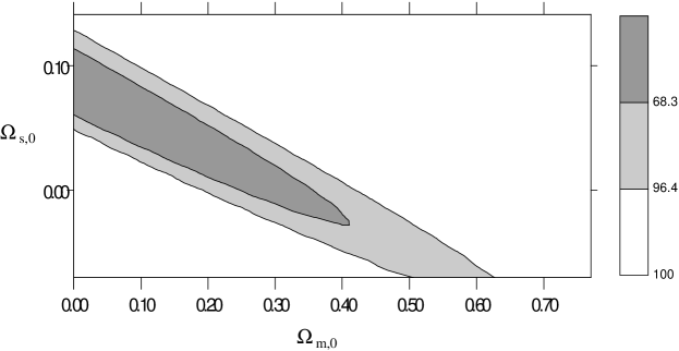
Figure 4: Confidence levels on the plane $(\Omega_{\text{m},0},\Omega_{\text{s},0})$ minimized over $\mathcal{M}$ for the flat model, and with $\Omega_{\Lambda,0}=1-\Omega_{\text{m},0}-\Omega_{k,0}-\Omega_{\text{s},0}$. The figure shows the ellipses of the preferred value of $\Omega_{\text{m},0}$ and $\Omega_{\Lambda,0}$. The results prefer the positive value of $\Omega_{\text{s},0}$, while the negative values are allowed (i.e., spin fluid can exist).

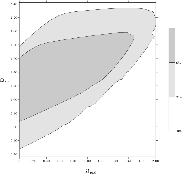
Figure 5: Confidence levels on the plane $(\Omega_{\text{m},0},\Omega_{\Lambda,0})$ minimized over $\mathcal{M}$, and with $\Omega_{\Lambda,0}=1-\Omega_{\text{m},0}-\Omega_{k,0}-\Omega_{\text{s},0}$. The figure shows the ellipses of the preferred values of $\Omega_{\text{m},0}$ and $\Omega_{\Lambda,0}$.

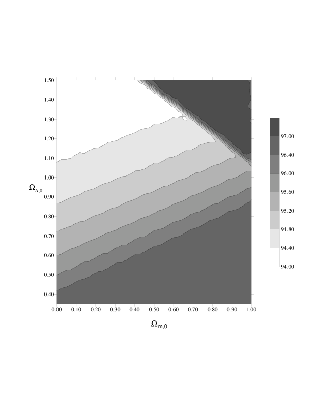
Figure 6: Levels of constant $\chi^{2}$ on the plane $(\Omega_{\text{m},0},\Omega_{\Lambda,0})$ marginalized over $\mathcal{M}$, and with $\Omega_{\Lambda,0}=1-\Omega_{\text{m},0}-\Omega_{k,0}-\Omega_{\text{s},0}$ The figure shows the preferred value of $\Omega_{\text{m},0}$ and $\Omega_{\Lambda,0}$.

Figure 7: The density distribution for $\Omega_{\text{s},0}$ in the model with spin effects ($\Omega_{\text{s},0}<0$) and brane effects ($\Omega_{\text{s},0}>0$). We obtain that $\Omega_{\text{s},0}>-0.012$ at the confidence level $1\sigma$ and $\Omega_{\text{s},0}>-0.026$ on the confidence level $2\sigma$. For simplicity, we only mark limits for the spin side.

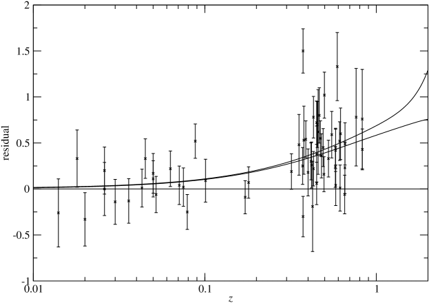
Figure 8: For $\Omega_{\text{m},0}=0.3$, residuals between the Einstein-de Sitter model and three cases: the Einstein-de Sitter itself (zero line), the $\Lambda$CDM flat model (middle curve), and the flat model with spin matter for $\Omega_{\text{s},0}=-0.012$ (highest curve).

The angular diameter of a galaxy is defined as

$$\theta=\frac{d(z+1)^{2}}{d_{L}}$$

where $d$ is the linear size of a galaxy. In the standard cosmology the flat dust-filled universe $\theta$ has the minimum value $z_{\text{min}}=5/4$. From Fig. 9 we can see that, if the spin matter is present, its influence on the predicted $\theta$ is weak. Theoretically it is possible to test values of $\Omega_{\text{s},0}$ from the angular diameter minimum value test. But because of evolutionary effects and observational difficulties the predicted differences are too small to be detected.

Figure 9: The angular diameter $\theta$ for the flat model with spin for $\Omega_{\text{m},0}=0.3$ and $\Omega_{\text{s},0}=0.1,0,-0.005$ (top, middle, bottom, respectively). The minima for these cases are $1.04$, $1.605$, no minimum, respectively. The spin causes the minimum to move right (toward higher $z$) and the minimum value of $\theta$ decreases.

Now let us briefly discuss the effect of spin fluid on the age of the Universe which is given by

$$t_{0}=\frac{1}{3H_{0}\sqrt{\Omega_{\Lambda,0}}}\ln\frac{2\Omega_{\text{m},0}+2\Omega_{\Lambda,0}+\sqrt{\Omega_{\Lambda,0}}}{\sqrt{\Omega_{\text{m},0}^{2}-4\Omega_{\text{s},0}\Omega_{\Lambda,0}}}.$$

In Fig. 10 we plot the age of the Universe in Gyr for the flat model for different $\Omega_{\text{s},0}$. Taking $\Omega_{\text{m},0}=0.3$ we obtain for $\Omega_{\text{s},0}=-0.013$: $t_{0}=13.347$, and for $\Omega_{\text{s},0}=0$: $t_{0}=14.436$. We can see that the spin fluid lowers significantly the age of the Universe. The cosmological constant is still needed to explain the problem of the age of the Universe.

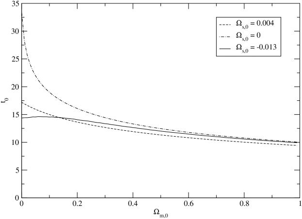
Figure 10: The dependence of the age of the universe $t_{0}$ (in units of $10^{9}$ yr) on the parameter $\Omega_{\text{m},0}$ for the flat model with spin fluid.

VI CMB peaks in the model with spin fluid

The cosmic microwave background (CMB) peaks arise from acoustic oscillations of the primeval plasma. Physically these oscillations represent hot and cold spots. Thus, a wave that has a density maximum at the time of last scattering corresponds to a peak in the power spectrum. In the Legendre multipole space this corresponds to the angle subtended by the sound horizon at the last scattering. Higher harmonics of the principal oscillations which have oscillated more than once correspond to secondary peaks.

For our end it is very important that the locations of these peaks are very sensitive to the variations in the model parameters. Therefore, it can serve as a sensitive probe to constrain the cosmological parameters and discriminate among various models.

The locations of the peaks are set by the acoustic scale $l_{A}$ which can be defined as the angle $\theta_{A}$ subtended by the sound horizon at the last scattering surface. The acoustic scale $l_{A}=\pi/\theta_{A}$ in the flat model is given by

$$l_{A}=\pi\frac{\int_{0}^{z_{\text{dec}}}\frac{dz^{\prime}}{H(z^{\prime})}}{\int_{z_{\text{dec}}}^{\infty}c_{s}\frac{dz^{\prime}}{H(z^{\prime})}}$$

where

$$H(z)=H_{0}\sqrt{\Omega_{\text{r},0}(1+z)^{4}+\Omega_{\text{s},0}(1+z)^{6}+\Omega_{\text{m},0}(1+z)^{3}+\Omega_{\Lambda,0}}$$

and $c_{s}$ is the speed of sound in the plasma (we assume additionally the presence of radiation in the model). The sound velocity can be calculated from the formula

$$c_{s}^{2}\equiv\frac{dp_{\text{eff}}}{d\rho_{\text{eff}}}=\frac{6\Omega_{\text{s},0}(1+z)^{3}+\frac{4}{3}\Omega_{\gamma,0}(1+z)}{3\Omega_{\text{m},0}+4\Omega_{\gamma,0}(1+z)+6\Omega_{\text{s},0}(1+z)^{3}}.$$

In the model of primeval plasma, there is a simple relation

$$l_{m}\approx l_{A}(m-\phi_{m})$$

between the location of $m$-th peak and the acoustic scale Doran et al. (2001); Hu et al. (2001). The prior assumptions in our calculations are as follows $\Omega_{\text{r},0}=9.89\times 10^{-5}$, $\Omega_{\text{b},0}=0.05$, and the spectral index for initial density perturbations $n=1$, and $h=0.65$.

The phase shift is caused by the prerecombination physics (plasma driving effect) and, hence, has no significant contribution from the term containing spin in that epoch. Because of above assumptions the phase shift $\phi_{m}$ can be taken from standard cosmology Hu et al. (2001)

$$\phi_{m}\approx 0.267\left[\frac{r(z_{\text{dec}})}{0.3}\right]^{0.1}$$

where $\Omega_{\text{b},0}h^{2}=0.02$, $r(z_{\text{dec}})\equiv\rho_{\text{r}}(z_{\text{dec}})/\rho_{\text{m}}(z_{\text{dec}})=\Omega_{\text{r},0}(1+z_{\text{dec}})/\Omega_{\text{m},0}$, $\Omega_{\text{r},0}=\Omega_{\gamma,0}+\Omega_{\nu,0}$, $\Omega_{\gamma,0}=2.48h^{-2}\times 10^{-5}$, $\Omega_{\nu,0}=1.7h^{-2}\times 10^{-5}$, $r(z_{\text{dec}})$ is the ratio of radiation to matter densities at the surface of last scattering.

The influence of spin on the location of the peaks is to shift them towards higher values of $l$. For example, for $\Omega_{\text{m},0}=0.3$, $\Omega_{\text{b},0}=0.05$, $h=0.65$, the different choices of $\Omega_{\text{s},0}$ yield the following

$$\Omega_{\text{s},0} =10^{-10}\colon l_{\text{peak},1} =186, l_{\text{peak},2}=441$$

$$\Omega_{\text{s},0} =1.4\times 10^{-10}\colon l_{\text{peak},1} =223, l_{\text{peak},2}=530$$

On the other hand from the Boomerang observations de Bernardis et al. (2002) we obtain $l_{\text{peak},1}=200-223$, $l_{\text{peak},2}=509-561$. Therefore, uncertainties in values $l_{\text{peak}}$ can be used in constraining cosmology with spin fluid, namely

$$10^{-10}\leq|\Omega_{\text{s},0}|\leq 1.4\times 10^{-10}$$

from the location of the first peak.

VII BBN in the model with spin fluid

We consider the non-relativistic matter with density $\rho$. In this case the spin effects scale like $-(1+z)^{6}$. It is clear that such a term can lead to accelerated expansion and the detailed analysis of supernovae Ia data requires it to be very subdominant today.

However, going back in time to the big bang nucleosynthesis (BBN) period, the term $\Omega_{\text{s},0}=-0.012$ would be dominant at redshift $z\gtrsim 2$. In such a model, radiation domination would never occur and all the BBN predictions would be lost. In practice, the preferred value obtained from SN Ia data gives the term $\rho_{\text{s}}^{2}$ which is far too large to be compatible with the BBN which is very well tested area of cosmology and does not allow for significant deviation from the standard expansion law, apart from very early times before the onset of the BBN. The consistency with the BBN seems to be crucial issue in spin fluid cosmology Arkani-Hamed et al. (1999); Binetruy et al. (2000). For this reason, not to suffer from the contradiction with the BBN, the contribution of spin fluid $\Omega_{\text{s},0}$ cannot dominate over the standard radiation term before the onset of BBN, i.e., for $z\cong 10^{8}$

$$-\Omega_{\text{s},0}(1+z)^{6}<\Omega_{\text{r},0}(1+z)^{4}\quad\text{and}\quad-\Omega_{\text{s},0}<10^{-20}.$$

Therefore, the term $\Omega_{\text{s},0}(1+z)^{6}$, describing the spin effects, is constrained by the BBN because it requires the change of expansion rate due to this term to be sufficiently small, so that an acceptable helium-4 abundance is produced.

VIII Conclusions

We discussed dynamics of the FRW model with spin fluid called the Weyssenhoff fluid. We showed that the effect of spin fluid is equivalent to fictitious fluid with equation like the Zeldovich stiff matter and negative energy density.

The dynamics of these models was analyzed on the two-dimensional phase plane and the Hamiltonian formalism was adopted to analyze all evolutional paths in the configuration space.

The dynamics determines the luminosity distance relationship which is used to test the models using the supernovae type Ia observations. It is shown that the presence of spin fluid matter has no influence on the present acceleration rate of the universe, and it is not an alternative to the cosmological constant description of dark energy.

We showed that the difference between the $\Lambda$CDM model and the model with spin fluid would be detectable if the content of spin fluid matter was sufficiently large, e.g., $\Omega_{\text{s},0}=-0.012$. This is possible because supernovae with redshift $z>1$ should be fainter in the model with spin fluid than in the $\Lambda$CDM model.

The detailed statistical analysis of supernovae data of sample A (analysis of confidence levels, levels of constant $\chi^{2}$ and density distribution of probability) was performed. From this analysis we obtained the limit of the density parameter for spin fluid $\Omega_{\text{s},0}$. At the confidence level of $1\sigma$ it is equal to $-0.012$.

We also applied the test of the minimum of the angular size of galaxies and showed that it is sensitive to the amount of spin fluid matter but difficult to detect. We found that the the presence of spin fluid matter lowers the age of the Universe.

Moreover we demonstrated that the stronger limit can be obtained from the CMB peak locations using the Boomerang data. From the uncertainties of the location of first peak we obtained a small interval for the values of spin fluid parameter $-1.4\cdot 10^{-10}\leq\Omega_{\text{s},0}\leq-10^{-10}$.

We find the formal analogy between the model with spin fluid and the brane model with dust on a brane. In both cases the dynamics equations are formally equivalent. In the early Universe these two kinds of matter scaled according the same law. For this reason we also considered the positive values of the spin fluid parameter $\Omega_{\text{s},0}$. From the statistical analysis we observed that a positive value of spin fluid parameter (brane) is most probable, nevertheless a negative value of this parameter is statistically allowed.

In the near future new high-redshift SN Ia observations will bring on better data. We expect that they will allow us to obtain the estimation of $\Omega_{\text{s},0}$ with a significantly lower error and to restrict the limit for spin fluid. In such a case the estimation of $\Omega_{\text{s},0}$ using SN Ia data will be worth reconsideration because this method does not depend on model assumptions, while the BBN limit on $\Omega_{\text{s},0}$ is strongly model dependent.