Consistent distances from Baade-Wesselink analyses of Cepheids and RR Lyraes

Abstract

By using the same algorithm in the Baade-Wesselink analyses of Galactic RR Lyrae and Cepheid variables, it is shown that, within $0.03$ mag $1\sigma$ statistical error, they yield the same distance modulus for the Large Magellanic Cloud. By fixing the zero point of the color–temperature calibration to those of the current infrared flux methods and using updated period–luminosity–color relations, we get an average value of $18.55$ for the true distance modulus of the LMC.

1 Introduction

A large number of papers have been published lately on the determination of the distance to the Large Magellanic Cloud (LMC). This increased interest is attributed to the extreme values published after the analyses of the hipparcos data on Cepheids (Feast & Catchpole 1997) and to the application of the red clump stars of the LMC through the same type of Galactic stars calibrated by hipparcos (Stanek et al. 2000). Along this line, there seems to exist a general belief that Cepheids yield usually longer distances (distance moduli of about $18.5$ mag and above), whereas RR Lyrae stars give shorter ones ($\approx 18.3$ mag). This latter belief is based on statistical parallaxes (Popowski & Gould 1998), Baade-Wesselink (BW) analyses (see Clementini et al. 1995, and references therein, hereafter C95) and the application of the hipparcos data (Fernley et al. 1998; see however Groenewegen & Salaris 1999). It is important to note that distances derived from the statistical parallax method employ rather small sample of stars ($\approx 200$ objects), whereas the hipparcos parallaxes for RR Lyrae stars are very inaccurate. Actually, more precise HST parallaxes yield distances in good agreement with the ”canonical” LMC value of $18.5$ mag derived from both prototype variables RR Lyr and $\delta$ Cep (Benedict et al. 2002a,b). It is also important to mention that all results based on the pulsation analyses of double-mode variables (RR Lyrae, Cepheids, both fundamental & first overtone and first overtone & second overtone ones) give basically the canonical value for the LMC distance (see Kovács 2002 and references therein).

In the light of the above, it is important to address the question of consistency between the BW analyses of Cepheids and RR Lyrae stars. Previous works have been performed by different groups of researchers, often using different BW parameters (e.g., $p$ factors, the ratio of the observed and surface radial velocities) and effective temperature relations (surface brightness for Cepheids – e.g., Laney & Stobie 1994, stellar atmosphere models for RR Lyrae stars – e.g., Liu & Janes 1990). In addition, there is a role of the somewhat delicate nature of the numerical method employed in the actual implementation of the BW analysis (e.g., computation of the surface acceleration). Therefore, we decided to visit the problem by using the same BW algorithm for both groups of stars. In order to compute the LMC distance modulus, the derived absolute magnitudes will be used in conjunction with currently published Period-Luminosity-Color (PLC) relations (Udalski et al. 1999; Kovács & Walker 2001, hereafter U99 and KW01, respectively).

2 Implementation of the BW method

Here we basically follow the standard methodology of the BW analysis as usually implemented in RR Lyrae studies (e.g., Liu & Janes 1990). In brief, we use the observed $V$ light, $V-K$ color and $V_{\rm rad}$ radial velocity curves to compute the luminosity ($L$), effective temperature ($T_{\rm eff}$) and radius ($R$) variations. For any assumed value of the equilibrium test radius $R_{0}$ we compute the following quantities:

• Temporal radius:

  • $R(t)=R_{0}+\Delta R(t)$,

  • $\Delta R(t)=-p\int_{0}^{t}[V_{\rm rad}(\tau)-\langle V_{\rm rad}\rangle]d\tau$,

  • $\langle V_{\rm rad}\rangle=P_{0}^{-1}\int_{0}^{P_{0}}V_{\rm rad}(\tau)d\tau$,

  where $P_{0}$ denotes the period, $p$ is the velocity projection factor, that we assume to be constant and set equal to $1.35$. (We note that Gieren, Fouqué & Gómez 1997 used a period-dependent $p$ factor. Their values span the range of 1.35–1.37 in the period regime of our sample. The effect of using lower $p$ is minute, because an increase of $0.02$ in $p$ yields an absolute magnitude that is brighter only by $0.02$ mag.)

• Temporal $T_{\rm eff}$:

  • $\log T_{\rm eff}=f[(V-K)_{0},{\rm[Fe/H]},\log g]$,

  where $f[...]$ denotes the interpolation polynomial of the stellar atmosphere models of Castelli, Gratton & Kurucz (1997) with the zero point determined by the scale of Blackwell & Lynas-Gray, (1994) (hereafter BLG94). The models have been computed without convective overshooting. The microturbulent velocity has been fixed at 2 km s^-1. The distribution of heavy elements follows that of the Sun. In order to find the temperature zero point offset between the model values of Castelli et al. (1997) and the ones given by the infrared flux method of BLG94, the compilation of the observational data on non-variable stars by C95 is used. We get $\log T_{\rm eff}$(model)$-\log T_{\rm eff}$(BLG94)$=0.0036$.

  It is interesting to compare this temperature scale with the one implied by the surface brightness (SB) method of Fouqué & Gieren (1997). Rewriting their formula given for the apparent angular diameter, we get $\log T_{\rm eff}=-0.131(V-K)_{0}-0.1BC+3.9474$. By using the above mentioned compilation of C95, we get an average difference of $\log T_{\rm eff}$(SB)$-\log T_{\rm eff}$(model& BLG94)$=-0.0035$. By performing the same test on the BW samples (see Table 1), the differences are positive, but less than $\approx 0.002$ for Cepheids. For RR Lyrae stars, the differences are even smaller, with changing signs. The larger negative difference on the sample of C95 is due in part to the larger weight of the higher temperature stars. In conclusion, we may state that the present temperature scale in the temperature range of interest is very similar to the ones used in earlier BW studies of Cepheids.

  For RR Lyrae stars, the iron abundance [Fe/H] is computed from the Fourier decompositions of the $V$ light curves as given by Jurcsik & Kovács (1996). For Cepheids, we set [Fe/H]$=$0, which seems to be a reasonable first approximation (see Luck et al. 2003 for the metallicity distribution of Cepheids). The temporal gravity $g$ is computed by $g=GM/R^{2}-p\thinspace dV_{\rm rad}/dt$, where $G$ is the gravitational constant, $M$ is the stellar mass, which is fixed at $0.7M_{\sun}$ and $5.0M_{\sun}$ for RR Lyrae stars and Cepheids, respectively. Since the contribution of $\log g$ to $\log T_{\rm eff}$ is relatively small when the $V-K$ color index is used, the exact value of $M$ is not crucial. In principle, we can compute a consistent value for $M$ by using the pulsation equation (e.g., van Albada & Baker 1973). However, both the weak dependence of $\log T_{\rm eff}$ on $\log g$, and the difference between the equilibrium and static stellar parameters (see Bono, Caputo & Stellingwerf 1995) make this procedure less straightforward and therefore, is left for the task of future studies. The dereddened color index $(V-K)_{0}$ is computed from the observed one by using $E_{B-V}$ reddening values either as given in the Galactic Cepheid Database of the David Dunlap Observatory or by the corresponding formula of KW01 for RR Lyrae stars. Because of the large reddenings of the Galactic Cepheids, we use the formulae for selective absorption ratios as given by the BW studies of Cepheids (see, e.g., Gieren, Fouqué & Gómez 1998):

  • $R_{V}=3.07+0.28(B-V)_{0}+0.04E_{B-V}$,

  • $R_{I}=1.82+0.205(B-V)_{0}+0.022E_{B-V}$,

  • $R_{K}=0.279$,

  • $A_{V}=R_{V}E_{B-V}$, $A_{I}=R_{I}E_{B-V}$, $A_{K}=R_{K}E_{B-V}$,

  where the $I$ and $K$ colors are in the Kron-Cousins and standard Johnson systems, respectively. For compatibility, these reddening relations are used also for RR Lyrae stars.

• Temporal absolute $V$ magnitude:

  • $M_{V}=-2.5\log L+M_{\rm bol}^{\sun}-BC(\log T_{\rm eff},{\rm[Fe/H]},\log g)$,

  • $\log L=4\log T_{\rm eff}/T_{\rm eff}^{\sun}+2\log R/R_{\sun}$,

  where $R_{\sun}$ and $T_{\rm eff}^{\sun}$ are the solar values. The latter one and the solar bolometric magnitude $M_{\rm bol}^{\sun}$ are set equal to $5778$ K and $4.75$ mag, respectively. The temporal bolometric correction $BC$ is computed from stellar atmosphere models in the same way as $\log T_{\rm eff}$ above. The zero point of $BC$ is set to a value which yields $BC_{\sun}=-0.07$.

• Point-by-point and average distance moduli:

  • $DM(i)=V(i)-R_{V}E_{B-V}(i)-M_{V}(i)$,

  • $\langle DM\rangle=N^{-1}\sum_{i=1}^{N}DM(i)$,

  • $\sigma_{DM}^{2}=(N-1)^{-1}\sum_{i=1}^{N}[DM(i)-\langle DM\rangle]^{2}$,

  where $N$ is the number of data points on the light curve.

The best fit is obtained at the test radius $R_{0}$ which yields the smallest $\sigma_{DM}$. Usually the fits are fairly accurate, with $\sigma_{DM}=0.02$–$0.01$. It is also worth mentioning the following technical details:

• When straightforward Fourier fitting does not work, smooth light and velocity curves are obtained through Fourier decompositions of the high order polynomials fitted by least squares to the observed data points of the folded light curves.

• Tables of stellar atmosphere models are employed through quadratic interpolation.

• All pulsation phases are used, including also the possibly shock-disturbed quick expansion phase.

• In spite of the careful treatment of the numerical derivation of the radial velocity curve, the total gravitational acceleration occasionally reaches values which lie outside the tabulated values. In these brief moments of pulsation the closest extreme values as given in the tables are used. The same method is employed for filtering out the non-tabulated values of $T_{\rm eff}$. We note that these out-of-range errors occur almost always out of the minimum of $\sigma_{DM}$, where the assumed unphysical stellar radius further enhances the numerical problems related to $\log g$.

3 PLC relations

Once the optimum equilibrium stellar parameters are computed by the above BW technique, we can evaluate the zero points of the corresponding PLC relations. Both for Cepheids and for RR Lyrae stars the PLC relations have been derived from stellar populations different from the Galactic BW samples. In the case of RR Lyrae stars there is a reasonable large overlap between the metallicities of the present BW sample and the cluster variables used by KW01 to derive the empirical formula. Therefore, we may assume that the formula may also be valid for most of the field variables used in the BW analysis. There is also a dispute on the possible metal dependence of the zero point of the Cepheid PLC relation. However, we think that there are more theoretical and empirical results which indicate the non-existence of such a dependence (Alibert et al. 1999; Bono et al. 2002; Turner & Burke 2002).

In the case of Cepheids we need to evaluate $C_{VI}$ in the following equation

$$\langle I_{c}\rangle-1.55(\langle V\rangle-\langle I_{c}\rangle)=-3.300\log P_{0}+C_{VI}\hskip 8.53581pt,$$ (1)

where $I_{c}$ denotes the Kron-Cousins colors, $\langle...\rangle$ means intensity-averaged magnitudes. The above formula has been derived by U99 for LMC with $C_{VI}=15.868$. Since the left-hand-side of Eq. (1) is reddening-free, the difference of $C_{VI}$(LMC) and the average of this constant for the BW stars will yield the true distance modulus for the LMC.

The PLC relation for the fundamental mode RR Lyrae stars is given by KW01

$$\overline{V}-3.1(\overline{B}-\overline{V})=-2.467\log P_{0}+C_{BV}\hskip 8.53581pt,$$ (2)

where the bars denote simple magnitude averages. The constant for LMC could be evaluated from the current $V$, $B$ observations of fundamental mode RR Lyrae stars in the LMC by Clementini et al. (2003, hereafter C03). Because they give intensity-averaged magnitudes, to retain compatibility with Eq. (2), we transform these values to simple magnitude averages with the aid of the formulae of Kovács (2002). The average of the $A_{1}$ Fourier amplitude is set equal to $0.30$, in accordance with the value obtained from the analysis of the RRab stars in the corresponding macho fields (Alcock et al. 2003). In this way we get $\overline{V}=0.032+\langle V\rangle$ and $\overline{B}=0.058+\langle B\rangle$. With the observed average $P_{0}$, $\langle V\rangle$ and $\langle B\rangle$ of $0\aas@@fstack{d}58$, $19.366$ and $19.744$, respectively, we get $C_{BV}=17.56$. However, the average magnitudes computed by C03 for their two fields $A$ & $B$ differ by as much as $0.08$ mag in $V$, and $0.13$ mag in $B$. They attribute this difference to the effect of differential extinction. We checked this difference by computing the averages in macho fields #6 & #13, overlapping with fields $A$ & $B$ of C03. With a $4\sigma$ clipping we got $\langle V\rangle=19.311\pm 0.012$ (field #6, 317 stars) and $\langle V\rangle=19.313\pm 0.010$ (field #13, 262 stars). With these small standard deviations of the means, we can state that a difference in the order of $0.1$ mag is not probable between the two fields.

In order to get another estimate on $C_{BV}$ for the LMC, we use the data of Soszyński et al. (2002), which cover a large sample of RR Lyrae stars of the Small Magellanic Cloud (SMC) from the ogle database. By proceeding as above, from their average magnitudes and period of $\langle V\rangle=19.74$, $\langle B\rangle=20.10$, $\langle V_{0}\rangle=19.45$, $\langle B_{0}\rangle=19.73$ and $\langle P_{0}\rangle=0.59$, we get $C_{BV}(SMC)=18.01$ and $17.97$, depending on whether reddened or dereddened magnitudes are used. Although Eqs. (1) and (2) should, in principle be reddening-free, the above difference shows that the field-by-field reddening corrections applied by Soszyński et al. (2002) may not be completely consistent with our standard extinction ratio. Since the method of their differential reddening correction has already proved to be successful (at least in statistical sense, see U99), we adopt the value obtained by the use of their dereddened magnitudes. In computing the value of $C_{BV}$ for the LMC, we have to subtract the relative distance modulus between the LMC and SMC. From the PLC relations derived for Cepheids in the two clouds, U99 got a difference of $0.51$ mag, which, with the above preliminaries, yields our finally adopted value of $C_{BV}=17.46$ for the LMC.

4 LMC distances from BW absolute magnitudes and PLC relations

The necessary data on RR Lyrae stars have been gathered from the literature during our earlier investigations (see KW01 and also C95, for a full list of variables subjected to BW analyses in earlier studies). For Cepheids we turned to the database of the McMaster University and also to the radial velocity database of the Moscow University (see Gorynya et al. 1998). We utilized only the best data available on fundamental mode variables. When it was necessary, the Cepheid $I$ light curves published in the Johnson system were transformed to the Kron-Cousins system with the aid of the formula given by Caldwell & Coulson (1987). Occasionally, periods have been improved by using the program package mufran (see Kolláth 1990). The variables used in the present study together with their derived physical parameters are given in Table 1. (Effective temperatures have been computed from the cycle-averaged $V-K$ and $\log g$ values.) Three RR Lyrae stars (W Crt, SS Leo and AV Peg) have been excluded from the above sample in the subsequent analysis, because of their discrepant positions in the PLC relation. For similar reasons, we also excluded X Lac from the Cepheid sample.

Table 1: Derived physical parameters of the BW variables

RR Lyraes
Name	$\log P$	$T_{\rm eff}$	$R/R_{\sun}$	$M_{V}$	$C_{BV}$
SW And	$-0.354$	6702	$4.47$	$0.81$	$-1.09$
WY Ant	$-0.241$	6296	$6.10$	$0.52$	$-1.17$
X Ari	$-0.186$	6111	$6.85$	$0.43$	$-1.15$
RR Cet	$-0.257$	6420	$5.22$	$0.75$	$-0.98$
UU Cet	$-0.217$	6258	$6.25$	$0.48$	$-1.22$
W Crt	$-0.385$	6788	$4.90$	$0.56$	$-1.31$
DX Del	$-0.325$	6691	$4.62$	$0.75$	$-1.13$
SU Dra	$-0.180$	6293	$5.85$	$0.62$	$-0.94$
SW Dra	$-0.244$	6393	$5.43$	$0.68$	$-1.02$
RX Eri	$-0.231$	6383	$5.40$	$0.70$	$-0.98$
RR Gem	$-0.401$	6721	$4.60$	$0.74$	$-1.19$
TW Her	$-0.398$	6732	$4.55$	$0.76$	$-1.16$
RR Leo	$-0.344$	6458	$4.85$	$0.87$	$-0.93$
SS Leo	$-0.203$	6431	$6.80$	$0.16$	$-1.41$
TT Lyn	$-0.224$	6283	$5.72$	$0.66$	$-1.04$
V445 Oph	$-0.401$	6792	$4.03$	$0.96$	$-1.02$
AV Peg	$-0.409$	6836	$3.62$	$1.18$	$-0.78$
AR Per	$-0.371$	6833	$4.45$	$0.72$	$-1.22$
BB Pup	$-0.318$	6712	$4.40$	$0.87$	$-0.95$
W Tuc	$-0.192$	6316	$6.75$	$0.27$	$-1.26$
TU UMa	$-0.254$	6369	$5.75$	$0.57$	$-1.14$
UU Vir	$-0.323$	6543	$4.95$	$0.75$	$-1.06$
Cepheids
Name	$\log P$	$T_{\rm eff}$	$R/R_{\sun}$	$M_{V}$	$C_{VI}$
$\eta$ Aql	$0.856$	5675	$60.8$	$-4.04$	$-2.97$
TT Aql	$1.138$	5589	$76.8$	$-4.46$	$-2.61$
VY Car	$1.277$	5257	$112.8$	$-4.95$	$-2.85$
WZ Car	$1.362$	5208	$107.6$	$-4.78$	$-2.38$
V Cen	$0.740$	5684	$42.8$	$-3.28$	$-2.60$
VW Cen	$1.177$	4998	$89.2$	$-4.12$	$-2.50$
XX Cen	$1.040$	5483	$64.0$	$-3.96$	$-2.48$
$\delta$ Cep	$0.730$	5765	$44.0$	$-3.42$	$-2.71$
X Cyg	$1.214$	5291	$100.0$	$-4.72$	$-2.77$
X Lac	$0.736$	5815	$55.6$	$-3.98$	$-3.18$
CV Mon	$0.731$	5689	$40.0$	$-3.14$	$-2.59$
T Mon	$1.432$	5096	$145.6$	$-5.31$	$-2.83$
UU Mus	$1.066$	5512	$72.0$	$-4.24$	$-2.65$
U Nor	$1.102$	5696	$80.4$	$-4.67$	$-2.89$
BF Oph	$0.609$	5903	$36.8$	$-3.16$	$-2.77$
BN Pup	$1.136$	5475	$74.0$	$-4.26$	$-2.53$
RY Sco	$1.308$	5312	$98.8$	$-4.72$	$-2.52$
BB Sgr	$0.822$	5645	$50.0$	$-3.58$	$-2.70$
U Sgr	$0.829$	5741	$51.6$	$-3.75$	$-2.82$
WZ Sgr	$1.339$	5064	$125.6$	$-4.94$	$-2.72$
RY Vel	$1.449$	5363	$132.0$	$-5.41$	$-2.66$
RZ Vel	$1.310$	5210	$122.8$	$-5.07$	$-2.88$
SW Vel	$1.370$	5231	$114.0$	$-4.93$	$-2.53$
T Vul	$0.647$	5986	$38.4$	$-3.32$	$-2.67$
U Vul	$0.903$	5964	$55.2$	$-4.10$	$-2.90$

The corresponding PLC relations are shown in Figs. 1 and 2. The constants in Eqs. (1) and (2) have been derived from the BW absolute magnitudes and reddening-free colors. The straight lines represent these calibrated relations. It is seen that the empirical slopes of the PLC relations fit perfectly the BW data (please note the highly different scales of the two figures). This strong correlation is very comforting, since two, completely separate methods and datasets are compared (BW results, based on Galactic variables on one hand, and empirical results, based on LMC and globular cluster variables on the other). The standard deviations of the BW points around the straight lines are $0.104$ and $0.157$ for RR Lyraes and Cepheids, respectively. We recall that the corresponding empirical values are $0.041$ and $0.058$ (see KW01 and U99). The much smaller values of these empirical standard deviations show that the BW luminosities still suffer from large random errors as it follows from the delicate nature of the BW method.

Computation of the LMC distance modulus is straightforward from the above results. It is obtained simply by the subtraction of the corresponding constants in the BW and empirical relations. By using the results of Sect. 3, from the RR Lyrae sample we get $m-M=17.46+1.09=18.55$, whereas from the Cepheid sample we obtain $m-M=15.87+2.69=18.56$. Although these true distance moduli are magically close to each other, we have to keep in mind that they both have a statistical errors of $\approx 0.03$ mag. Nevertheless, it is clear that the often cited $0.2$–$0.3$ mag difference between the BW distances derived from the two groups of variables no longer exists. They both yield the same distance within a relatively small statistical uncertainty.

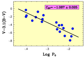
Figure 1: PLC relation for the 19 fundamental mode RR Lyrae stars listed in Table 1. The straight line corresponds to Eq. (2) with the adjusted constant given in the upper right box.

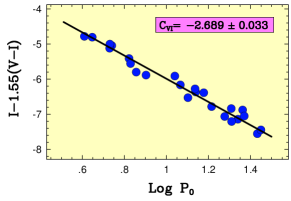
Figure 2: PLC relation for the 24 fundamental mode $\delta$ Cephei stars listed in Table 1. The straight line corresponds to Eq. (1) with the adjusted constant given in the upper right box.

It is interesting to compare the absolute magnitudes obtained in the present study with those derived earlier in other BW works. With the 18 Cepheids common with the sample of Gieren at al. (1998), we get and average difference (ours-theirs) of $-0.003$ mag, with a standard deviation $\sigma$ of $0.160$ mag. A similar comparison with the absolute magnitudes given for $p=1.35$ in Table 21 of C95, yields $-0.162$ with $\sigma=0.094$. This considerable difference results in a proper shift in the RR Lyrae distance modulus and leads to a result which is consistent with the one derived from Cepheids. The fact that Gieren et al. (1998) derives a $0.09$ mag lower distance for the LMC, in spite of the same average luminosity, is suspected to be caused by the difference between the PLC we use and the PL they employ to compute the LMC distance.

We find also a good agreement if we compare our radii with those of Gieren et al. (1998). For the 18 common variables we get an average difference (ours-theirs) of $-0.4$ $R_{\sun}$ with $\sigma=6.3$ $R_{\sun}$. In terms of the relative radii these figures become $-0.04$% and $6.9$%, respectively.

We can also make a comparison with the results of long-baseline interferometric measurements for Cepheids. For the two variables $\delta$ Cep and $\eta$ Aql common with the samples of Nordgren et al. (2002) and Lane, Greech-Eakman & Nordgren (2002), we find a rather close agreement between the radii. By applying the necessary corrections due to the different $p$ factors, from the interferometric/radial velocity results we obtain the radii of $42\times 1.35/1.31=43R_{\sun}$ and $62\times 1.35/1.43=58R_{\sun}$ for $\delta$ Cep and $\eta$ Aql, respectively. These values are very close to our corresponding figures (see Table 1).

It is important to note that although all direct estimates based on double-mode variables yield LMC distance modulus in agreement with the present result (Kovács 2002), the indirect distances derived from globular cluster double-mode RR Lyrae (RRd) stars become higher by $\approx 0.1$ mag, if we use the same PLC for the LMC as in the present paper. Nevertheless, these revised distance moduli computed from the RRd populations of M15, M68 and IC4499 are still in the range of $18.54$–$18.61$, which range is consistent with the value based on the present BW analysis.

We mention the recent effort of Cacciari et al. (2000) in revisiting the BW analysis of RR Lyrae stars with updated physics. From their analysis of two stars they concluded that the derived luminosities were in agreement with the earlier results (meaning the continuance of the old discrepancy, however, see C03 for a different conclusion from the same work).

5 Conclusions

We have shown that by using exactly the same method and Baade-Wesselink parameters (e.g., velocity projection factor), fundamental mode RR Lyrae and Cepheid variables yield the same distance modulus for the Large Magellanic Cloud. This is in variance with the earlier common belief that the two groups of stars lead to significantly different distance estimates for the LMC. The higher luminosity obtained for the RR Lyrae stars in the present study is attributed to: (a) the more accurate consideration of phase-dependent bolometric correction, (b) the more precise computation of the temporal gravity, (c) the better numerical treatment of both the grids of stellar atmosphere models and the observed light and velocity curves. The good agreement between the Cepheid luminosities obtained in this and in the earlier works suggests that the above conditions have already been met in those studies.

Although clarification of important theoretical problems (such as the accurate conversion of the projected velocity to the photospheric value, or the application of dynamical atmosphere models rather than static ones) are still needed, and better agreement between various photometric data on LMC is still demanded, we think that the present result is encouraging and indicates the possibility of making progress either by increasing the sample size by more precise data, or by building dynamical atmosphere models.

References

- [1] Alcock, C. et al., The macho collab., 2003, submitted to ApJ
- [2] Alibert, Y. Baraffe, I., Hauschildt, P. & Allard, F., 1999, A&A, 344, 551
- [3] Benedict, G. F. et al., 2002a, AJ, 123, 473
- [4] Benedict, G. F. et al., 2002b, AJ, 124, 1695
- [5] Blackwell D. E., Lynas-Gray A. E., 1994, A&A, 282, 899 (BLG94)
- [6] Bono, G., Caputo, F. & Stellingwerf, R. F., 1995, ApJS, 99, 263
- [7] Bono, G., Groenewegen, M. A. T., Marconi, M. & Caputo, F. 2002, ApJ, 574, L33
- [8] Cacciari, C., Clementini, G., Castelli, F. & Melandri, F., 2000, ASP Conf. Ser., 203, 176
- [9] Caldwell, J. A. R. & Coulson, I. M., 1987, AJ, 93, 1090
- [10] Castelli F., Gratton R. G. & Kurucz R. L., 1997, A&A, 318, 841 (see also http://kurucz.harvard.edu)
- [11] Clementini, G. et al., 1995, AJ, 110, 2319 (C95)
- [12] Clementini, G. et al., 2003, AJ, 125, 1309 (C03)
- [13] Feast, M. W. & Catchpole, R. M., 1997, MNRAS, 286, L1
- [14] Fernley, J. et al., 1998, A&A, 330, 515
- [15] Fouqué, P. & Gieren, W. P., 1997, A&A, 320, 799
- [16] Gieren, W. P., Fouqué, P. & Gómez, M., 1997, ApJ, 488, 74
- [17] Gieren, W. P., Fouqué, P. & Gómez, M., 1998, ApJ, 496, 17
- [18] Gorynya, N.A., et al., 1998, Astronomy Letters, Vol. 24, No. 11 (see also http://www.sai.msu.su/groups/cluster/gcvs/).
- [19] Groenewegen, M. A. T. & Salaris, M., 1999, A&A, 348, L33
- [20] Jurcsik J., Kovács, G., 1996, A&A, 312, 111
- [21] Kolláth, Z., 1990, Occ. Techn. Notes Konkoly Obs., 1, http://www.konkoly.hu/staff/kollath/mufran.html
- [22] Kovács, G., 2002, ASP Conf. Ser., 265, 163
- [23] Kovács G., Walker A. R., 2001, A&A, 371, 579 (see also Erratum: A&A, 374, 264) (KW01)
- [24] Lane, B. F., Greech-Eakman, M. J. & Nordgren, T. E., 2002, ApJ, 573, 330
- [25] Laney, C. D. & Stobie, R. S., 1994, MNRAS, 266, 441
- [26] Liu, T. & Janes K. A., 1990, ApJ, 354, 273
- [27] Luck, R. E. et al., 2003, A&A, 401, 939
- [28] Nordgren, T. E., Lane, B. F., Hindsley, R. B. & Kervella, P., 2002, AJ, 123, 3380
- [29] Popowski, P. & Gould, A., 1998, ApJ, 506, 259
- [30] Soszyński I. et al., 2002, Acta Astron. 52, 369
- [31] Stanek, K. Z., Kaluzny, J., Wysocka, A. & Thompson, I., 2000, Acta Astr., 50, 191
- [32] Turner, D. G. & Burke, J. F., 2002, AJ, 124, 2931
- [33] Udalski, A. et al., 1999, Acta Astron., 49, 201 (see also erratum at http://www.astrouw.edu.pl/ogle) (U99)
- [34] van Albada, T. S. & Baker, N., 1973, ApJ, 185, 477