Iron abundance in the ICM at high redshift

Abstract

We present the analysis of the X–ray spectra of 18 distant clusters of galaxies with redshift $0.3<z<1.3$. Most of them were observed with the Chandra satellite in long exposures ranging from 36 ks to 180 ks. For two of the $z>1$ clusters we also use deep XMM–Newton observations. Overall, these clusters probe the temperature range $3\,\raise-2.0pt\hbox{\hbox to0.0pt{\hbox{$\sim$}\hss}\raise 5.0pt\hbox{$<$}\ }\,kT\,\raise-2.0pt\hbox{\hbox to0.0pt{\hbox{$\sim$}\hss}\raise 5.0pt\hbox{$<$}\ }\,8$ keV. Our analysis is aimed at deriving the iron abundance in the Intra Cluster Medium (ICM) out to the highest redshifts probed to date. Using a combined spectral fit of cluster subsamples in different redshift bins, we investigate the evolution of the mean ICM metallicity with cosmic epoch. We find that the mean Fe abundance at $\langle z\rangle=0.8$ is $Z=0.25^{+0.04}_{-0.06}\,Z_{\odot}$, consistent with the local canonical metallicity value, $Z\simeq 0.3\,Z_{\odot}$, within 1$\sigma$ confidence level. Medium and low temperature clusters ($kT<5$ keV) tend to have larger iron abundances than hot clusters. At redshift $\langle z\rangle\sim 1.2$ (4 clusters at $z>1$) we obtain a statistically significant detection of the Fe-K line only in one cluster ($Z>0.10Z_{\odot}$ at the 90% c.l.). Combining all the current data set from Chandra and XMM at $z>1$, the average metallicity is measured to be $\langle Z\rangle=0.21^{+0.10}_{-0.05}\,Z_{\odot}$ (1$\sigma$ error), thus suggesting no evolution of the mean iron abundance out to $z\simeq 1.2$.

1 INTRODUCTION

Spectroscopic observations in the X–ray band provide a powerful means to probe the metal content of the diffuse gas in groups and clusters of galaxies. Typical metallicity in the Intra–Cluster Medium (ICM) of rich clusters out to redshifts $z\raise-2.0pt\hbox{\hbox to0.0pt{\hbox{$\sim$}\hss}\raise 5.0pt\hbox{$<$}\ }0.4$, are close to the canonical value of $Z=0.3\,Z_{\odot}$ (Mushotzky & Loewenstein 1997; Fukazawa et al. 1998; Allen & Fabian 1998; Della Ceca et al. 2000; Ettori, Allen & Fabian 2001), whereas they are found to be somewhat higher (up to a factor of two) in moderate mass clusters and groups (Buote 2000; Finoguenov, Arnaud & David 2001; Davis, Mulchaey & Mushotzky 1999; but see Renzini 1997). These observations show clearly that a significant amount of the metals produced by supernovae are injected into the ICM, a process which is essentially completed by $z\sim 0.4$.

The presence of metals in the ICM is crucial for tracing the past history of star formation in cluster galaxies. Supernova explosions, which are the main contributor to metal enrichment, may also provide a significant source of heating for the ICM. A number of observations concerning the ICM X–ray scaling properties (see Ponman, Cannon & Navarro 1999; Rosati, Borgani & Norman 2002 and references therein; Vikhlinin et al. 2002) suggests that non–gravitational heating processes must have taken place in the past and significantly affected the thermodynamics of the diffuse gas (e.g. Tozzi & Norman 2001; Bialek, Evrard & Mohr 2001; Babul et al. 2002; Tornatore et al. 2003; Voit et al. 2002). Therefore, a knowledge of the metal content of galaxy clusters and its evolution, combined with a precise modeling of the star formation processes, allows one to estimate the total amount of energy supplied by supernova explosions (e.g., Pipino et al. 2002, and references therein) and, ultimately, to understand the interplay between the evolution of the hot diffuse baryons and of the cold gas locked in the stellar phase.

On the observational side, data from the ASCA and Beppo-SAX satellites have allowed us to trace the spatial distribution of metals for a fairly large number of clusters (e.g., White 2000; Finoguenov, David & Ponman 2000; Dupke & White 2000; De Grandi & Molendi 2001; Finoguenov et al. 2002.) Such studies have provided useful information on the connection between the ICM metal distribution, the dynamical status of the clusters and the stellar population which synthesized such metals. For instance, De Grandi & Molendi (2001) found evidence for Fe gradients in relaxed systems which show signatures of cooling cores (but see Lewis, Buote & Stocke 2003). By mapping the different distributions of Ne, Si, S and Fe, Finoguenov et al. (2000) argued that Type Ia SN provide a larger contribution than Type II SN to the enrichment of central regions of clusters. With the advent of the Chandra and XMM satellites, and their unprecedented sensitivity and angular resolution, these studies are now carried out in great detail (e.g., Tamura et al. 2001; Ettori et al. 2002; Gastaldello & Molendi 2002; Matsushita et al. 2002), and provide new strong constraints on the physics of the ICM, as well as its chemical properties.

Specifically, with Chandra and XMM deep pointings on distant clusters, one can investigate the evolution of chemical abundances beyond $z=0.5$, thus extending a previous analysis based on ASCA data, which has shown no significant evolution in the iron abundance out to $z\sim 0.4$ (Mushotzky and Loewenstein 1997; Matsumoto et al. 2000). By tracing the evolution of the global metal content of the ICM one obtains useful information on the epoch at which the last significant episode of star formation in cluster galaxies took place and enriched the diffuse baryons.

In this Paper, we measure iron abundances in the ICM from a sample of 18 distant clusters extracted from the Chandra and XMM archives. Most of the analysis is based on Chandra data (14 pointings for 17 targets); two additional XMM observations are used for two clusters at $z>1$, one of which (RXJ0849) was also targeted by Chandra. The whole sample covers the redshift range $0.3\raise-2.0pt\hbox{\hbox to0.0pt{\hbox{$\sim$}\hss}\raise 5.0pt\hbox{$<$}\ }z\raise-2.0pt\hbox{\hbox to0.0pt{\hbox{$\sim$}\hss}\raise 5.0pt\hbox{$<$}\ }1.3$ and includes clusters with temperature between 3 and 8 keV.

The plan of the Paper is as follows. In §2 we describe the data reduction procedure. In §3 we describe the spectral analysis of the single sources (§3.2), and of the combined spectra of subsamples (§3.3). In §4 we discuss possible implications of our findings and summarize our conclusions. We adopt a cosmological model with $H_{0}=70$ km/s/Mpc, $\Omega_{M}=0.3$ and $\Omega_{\Lambda}=0.7$ throughout. Quoted confidence intervals are 68% unless otherwise stated.

2 OBSERVATIONS AND DATA REDUCTION

2.1 Chandra data

In Table 1, we present the list of the Chandra observations analyzed in this Paper. Some of them are also part of the analysis presented by Ettori, Tozzi & Rosati (2003). Most the observations were carried out with ACIS–I, while for MS2137, MS1054 and MS0451 the Back Illuminated S3 chip of ACIS–S was also used. The data are reduced using the 2.3 version of the CIAO software (release V2.3, see http://cxc.harvard.edu/ciao/), and use the level=1 event file as a starting point. For observations taken in the VFAINT mode, we run the tool acis_process_events to flag probable background events using all the information of the pulse heights in a $5\!\times\!5$ event island (as opposed to a $3\!\times\!3$ event island recorded in the FAINT mode) to help distinguishing between good X–ray events and bad events that are most likely associated with cosmic rays. With this procedure, the ACIS particle background can be reduced significantly compared to the standard grade selection (see http://asc.harvard.edu/cal/Links/Acis/acis/Cal_prods/vfbkgrnd/). Real X–ray photons are practically not affected by such cleaning (only about 2% of them are rejected, independently of the energy band, provided there is no pileup).

We also apply the CTI correction (see http://cxc.harvard.edu/ciao/threads/acisapplycti/ when the temperature of the Focal Plane at the time of the observation was 153 K. This procedure allow us to recover the original spectral resolution partially lost because of charge transfer inefficiency (CTI). The correction applies only to ACIS–I chips, since the ACIS-S3 did not suffer from radiation damage.

If the data are taken in the FAINT mode, we run the tool acis_process_events only to apply the CTI correction and update the gain file with the latest version provided within CALDB to date (version 2.18). From this point on, the reduction is similar for both the FAINT and the VFAINT exposures. The data are filtered to include only the standard event grades 0, 2, 3, 4 and 6. We checked visually for hot columns left from the standard cleaning. We needed to remove hot columns by hand only in a few cases. We identify the flickering pixels as the pixels with more than two events contiguous in time, where a single time interval was set to 3.3 s. For exposures taken in VFAINT mode, there are practically no flickering pixels left after filtering out the bad events. We perform a final cleaning by filtering time intervals with high background by performing a 3–$\sigma$ clipping of the background level using the script analyze_ltcrv (see http://cxc.harvard.edu/ciao/threads/filter_ltcrv/). The removed time intervals always amount to less than 5% of the nominal exposure time for ACIS–I chips. We note however, that some observations show large flares on the ACIS–S3 chip, which are not removed by our analysis since they are not visible on the ACIS-I chips. We remark that our spectral analysis is not affected by such flares, since we always compute the background from the same observation (see below), thus taking into account any spectral distortion of the background itself induced by the flares.

All the observed clusters are detected with very high signal–to–noise. The spectrum of each source is extracted from a circular region around the centroid of the photon distribution. For each cluster we select the extraction radius according to the following criteria. For a given radius, we find the center of the region which includes the maximum number of net counts from the source in the 0.5–5 keV band. Then, we compute the signal–to–noise, repeating this procedure for a set of radii. Finally we choose the radius for which the 0.5–5 keV signal–to–noise is maximum. Incidentally, we notice that in all the cases the extraction radius defined by maximizing the S/N is roughly 3 times the core radius measured with a beta model (for the spatial analysis of these clusters see Ettori et al. 2003, in preparation). In addition, the fraction of the net counts included in our extraction regions is always between 0.80 and 0.90 of the total. Therefore, our choice of the extraction radius allows us to measure the global properties of the clusters using the majority of the signal with the highest signal–to–noise ratio, and it minimizes any scaling effect due to possible temperature and metallicity gradients which depend on the mass scale.

For each cluster, we use the events included in the extraction region to produce a spectrum (pha) file. The background is always obtained from regions of the same exposures (same chip where the source is located). This is possible since all the sources are less than 3–4 arcmin in extent. The background file is scaled to the source file by the ratio of the geometrical area. We checked that variations of the background intensity across the chip do not affect the background subtraction, by comparing the count rate in the source and in the background at energies larger than 8 keV, where the signal from the sources is null.

The response matrices and the ancillary response matrices are computed in a single position at the center of the cluster. We checked that the variation of the spectral response of the detector across the source position on the chip does not affect the result of the fit. When the source counts are spread on more than one node, we repeated the analysis node by node; however, we never found any change in the best–fit values. In general, the variation of the response matrix as a function of the position on the chip is affecting the spectral fits only for high signal–to–noise spectra, while, in our case, the statistical errors are always dominating.

2.2 XMM data

In Table 2 we list the two XMM–Newton observations included in our analysis, using the European Photon Imaging Camera (EPIC) PN and MOS detectors. We use XMM data to boost the signal–to–noise only for the most distant clusters in our current sample.

RXJ0849+4452 is the more luminous of the two $z\simeq 1.26$ clusters in the Lynx field (Rosati et al. 1999, Stanford et al. 2001). We have obtained calibrated event files for the MOS1, MOS2 and PN cameras with the XMM Standard Analysis System (SAS) routines (SASv5.3.3). Time intervals in which the background is increased by soft proton flares are excluded by rejecting all events accumulated when the count rates in the 10–12 keV band exceeds 40 cts/100s for the PN and 20cts/100s for each of the two MOS cameras. The final effective exposure time amounts to 60 ks for the PN and to 112 ks for the two MOS. Note that we do not use data from the less luminous $z>1$ cluster in the Lynx field, RXJ0848+4453, since it is barely detected in the XMM data due to the high background and confusion with faint field sources.

The cluster RXJ1053.7+5735 (Hashimoto et al. 2002), is located in the Lockman Hole field, which was observed with XMM during the Performance Verification phase of EPIC (Jansen et al. 2001; Hasinger et al. 2001; Mainieri et al. 2002). Here we use a redshift of $z=1.15$ from Hasinger et al. (2003 in preparation) which revises the initial value published by Thompson et al. (2001). The EPIC cameras were operated in the standard full–frame mode. The thin filter was used for the PN camera, and both thin and thick filters for the MOS1 and MOS2 cameras. The final effective exposure time, after removing background flares, is approximately 94 ks. RXJ1053, which is located at an off-axis angle of $\sim 10^{\prime}$, has a double–lobed morphology with the two cores 1 arcmin apart (see Hashimoto et al. 2002). We will present the analysis of the whole cluster, as well as the separate analyses of the two clumps, which show significantly different temperatures.

3 RESULTS

3.1 Spectral analysis

The spectra are analyzed with XSPEC v11.2.0 (Arnaud 1996) and fitted with a single temperature MEKAL model (Kaastra 1992; Liedahl et al. 1995), where the ratio between the elements are fixed to the solar value as in Anders & Grevesse (1989). These values for the solar metallicity have recently been superseded by the new values of Grevesse & Sauval (1998), who use a 0.676 times lower Fe solar abundance. However, we prefer to report metallicities in units of the Anders & Grevesse abundances since most of the literature still refers to these old values. Since our metallicity depends only on the Fe abundance, updated metallicities can be obtained simply by rescaling by 1/0.676 the values reported in Table 3. We model the Galactic absorption with tbabs (see Wilms, Allen & McCray 2000).

Before performing the fits, we apply a double correction to the arf files. We apply the script apply_acisabs by Chartas and Getman to take into account the degradation in the ACIS QE due to material accumulated on the ACIS optical blocking filter since launch (see http://cxc.harvard.edu/ciao/threads/apply_acisabs/). This correction applies to all the observations. For data taken with ACIS–I, we also manually apply a correction to the effective area consisting in a 7% decrement below 1.8 keV to homogenize the low–energy calibrations of ACIS–S3 and ACIS–I (see Markevitch & Vikhlinin 2001).

The fits are performed over the energy range 0.6–8 keV. We exclude photons with energy below 0.6 keV in order to avoid systematic biases in temperature determination due to uncertainties in the ACIS calibration at low energies. The effective cut at high energies can be lower than 8 keV, since the signal–to–noise for thermal spectra rapidly decreases at energies above 5 keV. Generally, we cut at 7–8 keV after visually inspecting each spectrum. The excluded energy range (0.3–0.6 keV for Chandra, and below 0.5 keV for XMM) does not affect the determination of the metallicity, which is dominated by the Fe K line complex at rest–frame energies of 6.4–6.7 keV (always located above $\sim$3 keV for our cluster sample). All the iron and oxygen L spectral features at 1 keV rest–frame are redshifted below 0.8 keV for $z\raise-2.0pt\hbox{\hbox to0.0pt{\hbox{$\sim$}\hss}\raise 5.0pt\hbox{$>$}\ }0.4$, i.e. for the majority of our sample. We note that our Fe K-line diagnostic is simpler and more robust than that based on the line–rich region around 1 keV, where the line emission is dominated by the L–shell transition of Fe, and the K–shell transitions of O, Mg, and Si.

We use three free parameters in our spectral fits: temperature, metallicity and normalization. We freeze the local absorption to the galactic neutral hydrogen column density ($N_{H}$, table 3), as obtained from radio data (Dickey & Lockman 1990), and the redshift to the value measured from the optical spectroscopy. Since both the absorption and the redshift can be in principle determined from the X–ray data itself, we checked that our results do not change when these parameters are left free, as described below.

A well-known strong degeneracy exists between $N_{H}$ and the best–fit temperature: a higher $N_{H}$ implies always a lower $kT$, with a rough scaling $N_{H}\propto T^{-4}$. We looked for a possible biases by comparing the best–fit values obtained after fixing the local absorption to the Galactic one, with those obtained using $N_{H}$ as a free parameter. An inspection of the contour plots in the Figures of Appendix A, shows that the Galactic values by Dickey & Lockman (1990) are typically recovered within the $1\sigma$ contours in the $N_{H}$–$T$ space, with three exceptions (MS2137, MS0451, MS1054), for which a discrepancy larger than $3\sigma$ is found. In addition, we also notice that the best–fit temperature is found in 3 cases somewhat higher than the value obtained for a free $N_{H}$, in 4 cases somewhat lower, while in the remaining 11 cases it is practically coincident. Therefore, we conclude that by fixing the local absorption to the Dickey & Lockman values, we do not introduce any significant systematic bias in the measure of the temperature.

We also checked that the best–fit temperature remains unaffected when the redshift is left free. The best–fit redshift is consistent with the spectroscopic redshift for most of the clusters within $1\sigma$, and between $1$ and $2\sigma$ in the remaining 3 cases (RXJ1113, RXJ1350, RXJ0849). Generally, small changes in the redshift can give significant changes in the best–fit metallicity, since its value depends critically on the position of the Fe line. We find that the metallicity tends to be higher when the redshift is left free. This is due to positive noise fluctuations which systematically tend to boost the Fe line equivalent width. It is evident that for such low signal–to–noise spectra the best strategy is to lock the cluster redshift to the spectroscopic value.

In performing the spectral fits we used the Cash statistics applied to source plus background (see http://heasarc.gsfc.nasa.gov/docs/xanadu/xspec/manual/node57.html), which is preferable for low signal–to–noise spectra (Nousek & Shue 1989). We also performed the same fits with the $\chi^{2}$ statistics (with a standard binning with a minimum of 20 photons per energy channel in the source plus background spectrum) and verified that all the best–fit models have a reduced $\chi^{2}\sim 1$.

3.2 Single source analysis

In this section, we present the results of the spectral analysis of the 18 clusters. We remind that RXJ0152 shows two distinct cores which we treat as separate objects. As for RXJ1053, the spatial separation of the two clumps is less clear. Therefore, we show the analyses of the whole cluster as well as that of the two clumps, which, indeed, have significantly different temperatures (Hashimoto et al. 2002). The results are listed in Table 3.

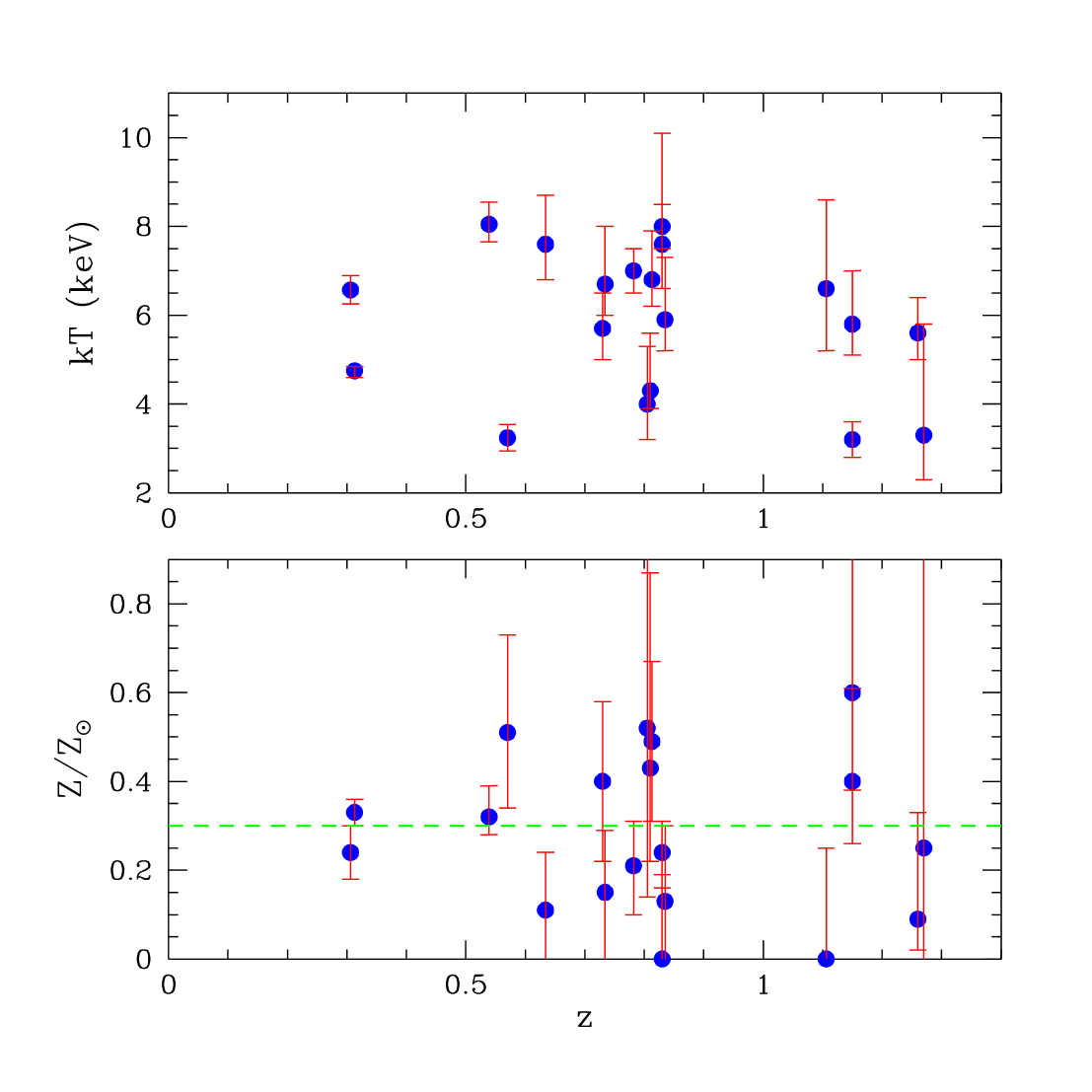
Figure 1: Temperature (upper panel) and Fe abundance (lower panel) vs redshift for the 18 clusters in the sample. Error bars refer to 1 $\sigma$ c.l. computed for one interesting parameters. The metallicity is given in units of the solar Fe abundance as measured by Anders & Grevesse (1989)

In Figure 1 we show the distribution of temperature and Fe abundance for our sample as a function of redshift (error bars are at $1\sigma$ confidence level). We looked for possible correlations between different parameters. For the temperature–redshift relation we find a Spearman’s rank coefficient of $r_{s}=-0.20$ for 19 degrees of freedom, thus consistent with no correlation. As for the metallicity–redshift relation, we find again no correlation, with Spearman’s rank coefficient of $r_{s}=-0.15$ for 19 degrees of freedom,

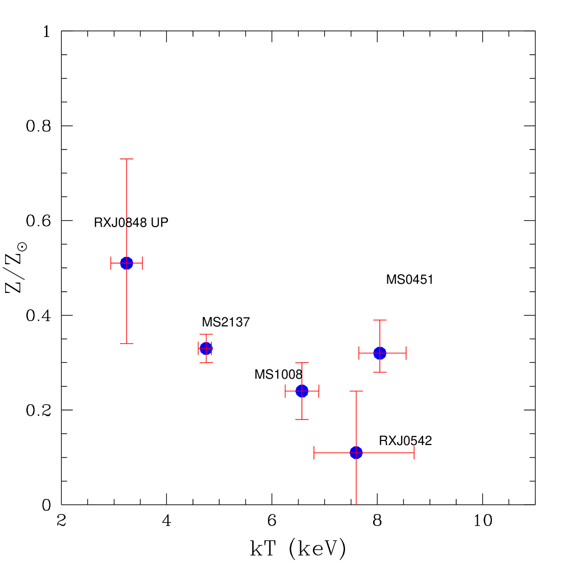
Figure 2: Temperature–metallicity plot for 5 clusters in the redshift range $0.3<z<0.65$. Error bars refer to 1 $\sigma$ c.l. for one interesting parameter. The metallicity is given in units of the solar Fe abundance as measured by Anders & Grevesse (1989).

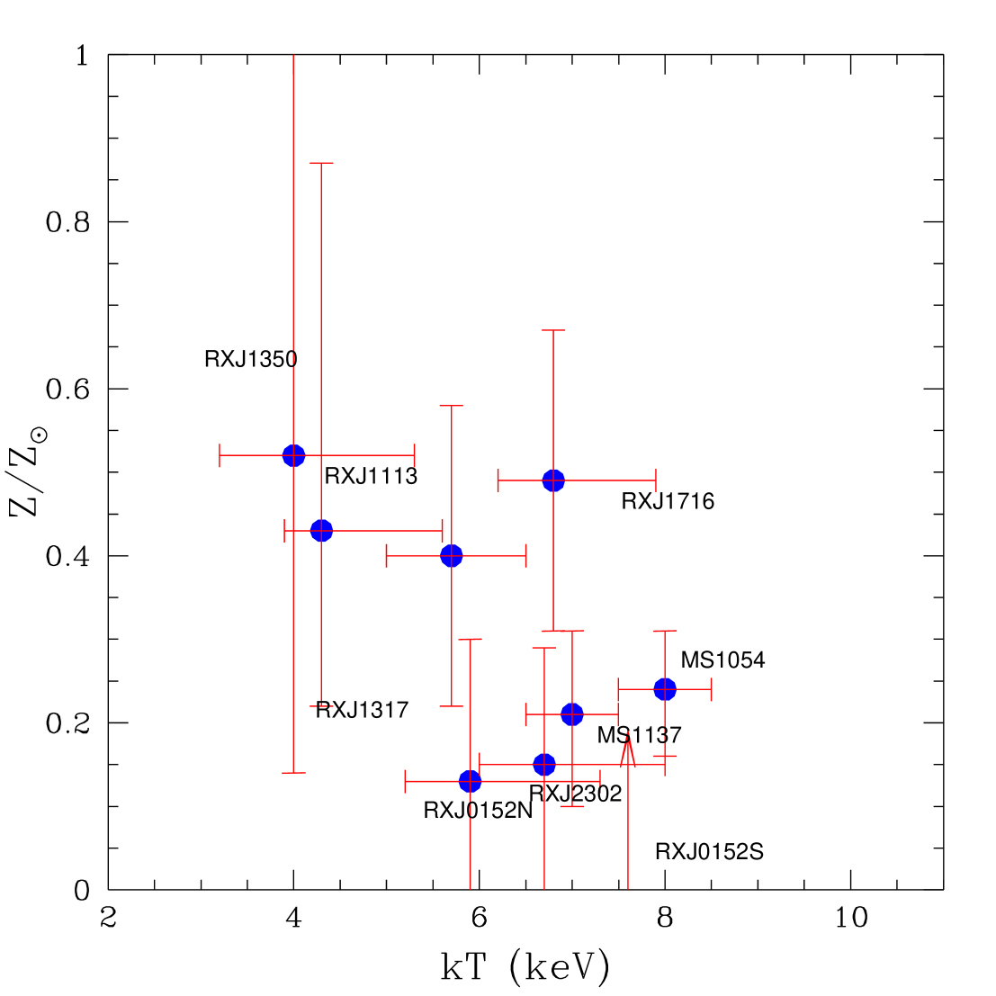
Figure 3: Same as in Figure 2 for 9 clusters in the redshift range $0.65<z<0.90$.

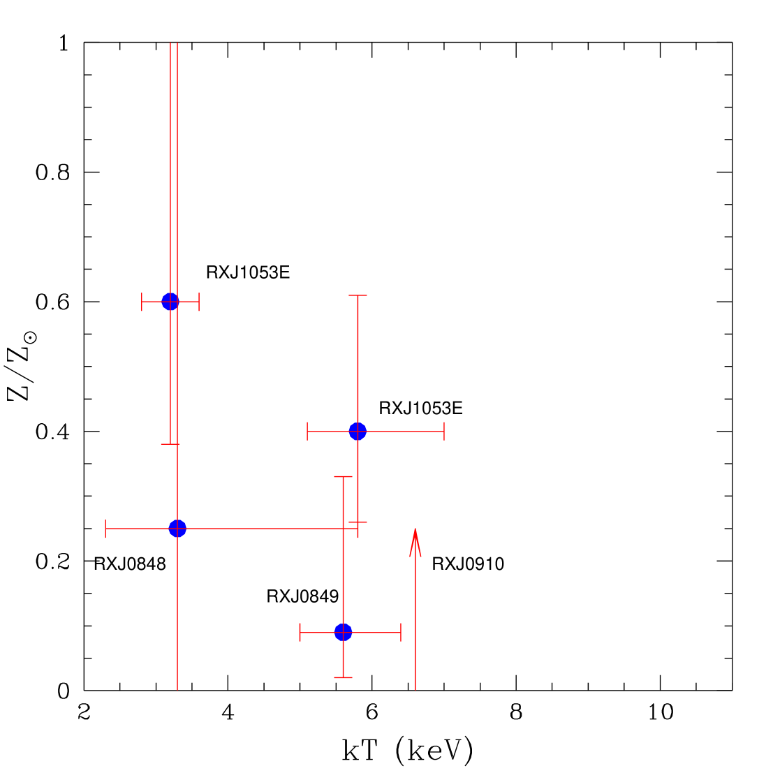
Figure 4: Temperature–metallicity plot in the redshift range $1.1<z<1.3$ for the 4 clusters observed with Chandra and XMM. We obtain a positive detection of the Fe abundance only for RXJ1053 (observed only with XMM), and upper limits for the other three clusters. Error bars refer to 1$\sigma$ c.l. for one interesting parameter. The metallicity is given in units of the solar Fe abundance as measured by Anders & Grevesse (1989).

We show our results for three redshift intervals: $0.3<z<0.65$ (five objects, Figure 2), $0.65<z<0.90$ (nine objects, Figure 3), $0.90<z<1.25$ (five objects, Figure 4). We notice a large intrinsic scatter, which is, however, comparable with the statistical errors. Given the small size and the limited temperature range of our sample, it is difficult to draw any conclusion on the relation between Fe abundance and temperature at a given redshift. We notice, however, a trend of lower Fe abundance at higher temperatures ($kT>5$ keV) with a Spearman’s correlation coefficient $r_{s}=-0.57$ for 19 degree of freedom, slightly below the 90% confidence level, for the whole sample. We find a Spearman’s correlation coefficient of $r_{s}=-0.70$, $r_{s}=-0.50$, and $r_{s}=-0.70$ for 5, 9 and 5 degrees of freedom respectively in the three redshift intervals. We note that the presence of such a correlation is in keeping with observations of local and moderate redshift clusters (see Mushotzky & Loewenstein 1997; Finoguenov, Arnaud & David 2001), which suggest higher Fe abundances for lower temperature systems. Given this result, we choose to differentiate our sample in low and high temperature clusters. If we compute the Fe abundance–redshift relation for the 13 clusters with $kT>5$ keV, we find a Spearman’s rank coefficient of $r_{s}=-0.40$ for 13 degrees of freedom, which at face value implies a correlation at $\raise-2.0pt\hbox{\hbox to0.0pt{\hbox{$\sim$}\hss}\raise 5.0pt\hbox{$<$}\ }2\sigma$ confidence level.

In the intermediate redshift bin ($0.65<z<0.90$), the Fe emission line is clearly detected in the average cluster population (see also §3.3), although the metallicity is consistent with zero (within 1 $\sigma$) for three clusters, and for one of them (RXJ0152S) we have only an upper limit. In the highest redshift bin ($z>1$, see Figure 4), the Fe K line is detected only in the spectrum of RXJ1053 (for which $Z>0.1\,Z_{\odot}$ at the 90% c.l.) as well as in the two separate clumps, which have different temperatures: $kT=3.2\pm 0.4$ keV for the eastern clump and $kT=5.8^{+1.2}_{-0.7}$ keV for the western clump. In the spectra of the other two clusters with $kT>5$ keV we do not detect the iron line. To investigate further the Fe abundance–redshift relation, we propose to measure the average metallicity of the ICM as a function of cosmic epoch by combining photons from subsamples of clusters as described below.

3.3 Combined spectral analysis

A robust measurement of the average ICM metallicity as a function of cosmic epoch can be obtained by combining the information contained in the individual spectra, after grouping them in a number of redshift bins. This technique is similar to the stacking analysis often performed in optical spectroscopy, where spectra from a homogeneous class of sources are averaged together to boost the signal–to–noise, thus allowing the study of otherwise undetected features. In this case, one cannot stack different spectra due to their different shapes (different temperatures), however one can perform a combined fit, as explained below.

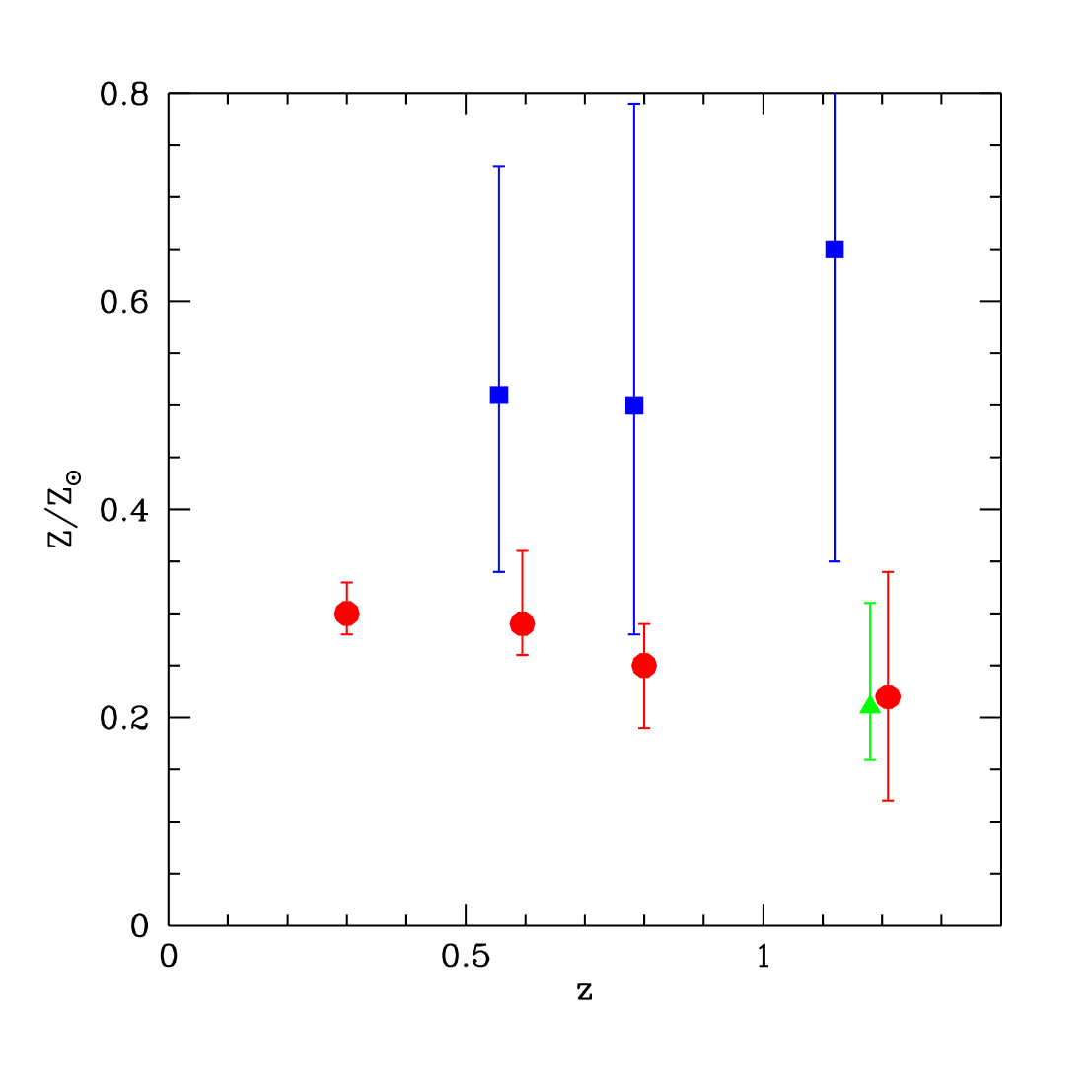
Figure 5: Average metallicity as a function of the redshift for the four bins defined in the text, for clusters with $kT>5$ keV (solid circles) and $kT<5$ keV (solid squares). For the highest redshift bin ($z\sim 1.2$), we have only an upper bound from the three clusters with $kT>5$ keV, while we measure the iron abundance only for RXJ1053 ($kT\simeq 4$ keV). The triangle is the combined fit of all the clusters at $z>1$ irrespective of the temperature. Error bars refer to $1\sigma$ c.l.

We define 4 redshift bins as follows. The first bin includes only MS1008 and MS2137 with $\langle z\rangle=0.31$; the second one includes MS0451, RXJ0848$-$4456 and RXJ0542, with $\langle z\rangle=0.57$; the third one includes 9 clusters: RXJ2302, RXJ1113, MS1137, RXJ1317, RXJ1350, RXJ1716, MS1054, RXJ0152N, RXJ0152S, with $\langle z\rangle=0.80$; the fourth one includes the five objects at $z>1$: RXJ0910, RXJ0849 (observed with Chandra and XMM), RXJ0848, and the two clumps of RXJ1053 in the Lockman Hole observed only with XMM. The average redshift in the highest–z bin is $\langle z\rangle\simeq 1.2$. In each redshift bin, we performed a combined fit, leaving temperature and normalization free for each object, using however a single metallicity parameter for all the clusters in the subsample. We also subdivide the clusters within each redshift bin according to temperature, below and above 5 keV, in order to investigate whether either low– or high–temperature clusters contribute to a possible evolution of the average metallicity. We show our results in Figure 5 (the best fit values are listed in Table 4).

We measure a mean metallicity very close to the canonical local value of $0.3Z_{\odot}$ out to $z\simeq 0.6$ for high temperature clusters. We have only one cluster with temperature below 5 keV at $z<0.6$ (RXJ0848+4456), for which we find $Z\sim 0.5\,Z_{\odot}$ with large error bars. More interestingly, we obtain for the first time a robust determination of the Fe mean abundance at $z=0.8$: $\langle Z\rangle=0.25^{+0.04}_{-0.06}$ in clusters with $kT>5$ keV, and possibly higher ($Z\simeq 0.5\,Z_{\odot}$) for lower temperature clusters. At $z>1$ the combined fit for the three $kT>5$ keV clusters yields a weak positive detection of $Z=0.22\pm 0.12\,Z_{\odot}$. This measure is consistent with the local value within one sigma. The two measures for with $kT<5$ keV (RXJ0910 and the eastern clump of RXJ1053) give a very large value for the iron abundance of $Z\simeq 0.6\,Z_{\odot}$, but with large uncertainties. If we combine all the clusters at $z>1$ irrespective of the temperature, we obtain $\langle Z\rangle=0.21^{+10}_{-0.05}$. This measure is dominated by RXJ1053, which contributes to the combined fit with 870 total net counts, while we have 1550 net counts from the remaining three clusters. This measure of the average iron abundance can be considered an average among clusters with different properties: if the other high–z clusters had the same metallicity, we would have been able to measure it.

The values of mean metallicity as a function of redshift can be fitted with a constant value: a $\chi^{2}$ minimization on the four points obtained for clusters with $kT>5$ keV gives $Z=0.286Z_{\odot}$ as the best choice ($\chi^{2}\sim 3$ for 3 degrees of freedom). As a result, we do not find significant evolution in the mean ICM metallicity out to $z\sim\!1.2$. The apparent decline of $\langle Z\rangle$ at $z>1$ in high–temperature clusters (Figure 5) has a very low confidence level (between 70% and 80%).

To better establish the statistical significance of our Fe abundance measurement in the highest redshift bin, as well as possible biases on its best–fit value, we performed simulations of the combined spectral analysis by creating synthetic spectra with the same signal–to–noise and global parameters ($L_{X},T,N_{H},z$) as our high–z clusters. We fixed the metallicity to be the same, $0.3Z_{\odot}$, in the 5 objects at $z>1$. We used XSPEC (fakeit command) to simulate source spectra and background spectra for each cluster starting from the actual value of the background derived from the data. We then ran 1000 simulation for each cluster and analyzed them with the same fitting procedure adopted on the real data to derive the average metallicity at redshift $z=1.2$ (we recall that the combined fit is performed on 6 separate spectra since for RXJ0849 we use 3 separate data sets: Chandra-ACIS, XMM–PN and XMM–MOS). We verified that the best–fit values for the temperatures for each cluster are distributed around their respective input values. In Figure 6, we show the distribution of the best–fit values for the metallicity from the combined fit of 1000 simulations (solid line). The distribution is rather broad, with a spike at zero metallicity (in 5% of the case), underlying the difficulty in constraining the metallicity at such high redshifts from an effective number of $\sim\!2400$ photons. The median value of the recovered best–fit metallicity is $Z=0.325\,Z_{\odot}$; the 84 lower percentile corresponds to $Z=0.13\,Z_{\odot}$, thus including our measured value of $Z\simeq 0.20\,Z_{\odot}$. In the simulations reproducing only the observations of clusters with $kT>5$ keV (dashed line) the 84 lower percentile corresponds to $Z=0.02\,Z_{\odot}$. These simulations show that in order to detect possible evolution of the average metallicity at $z>1.2$ in high temperature clusters, we need to enlarge substantially our sample.

4 DISCUSSION AND CONCLUSIONS

We presented the spectral analysis of 18 clusters of galaxies at intermediate–to–high redshifts observed by Chandra and XMM. Our analysis represents the first attempt to date to follow the evolution of iron content of the ICM out to $z\raise-2.0pt\hbox{\hbox to0.0pt{\hbox{$\sim$}\hss}\raise 5.0pt\hbox{$>$}\ }1$.

As a first firm result of our analysis, we determine the average ICM metallicity with a 20% uncertainty at $z<1$ ($Z/Z_{\odot}=0.25^{+0.04}_{-0.06}$ at $\langle z\rangle=0.8$) and find no evidence of evolution over this redshift range. This finding is consistent with the expectation that the peak of star formation in proto–cluster regions occur at redshift $z\simeq 3$–4. The extension of this analysis at $z>1$, with similar accuracy in the determination of the Fe abundance, will be very valuable and could further constrain the epoch at which the ICM was metal–enriched from the last significant episode of star formation.

Our sample includes only 4 clusters at $z>1$ to date. One of these clusters, RXJ1053, shows two clumps with different temperatures. In this way, we end up with three structures having $kT>5$ keV and two at lower temperature. A combined fit across the high temperature systems yields $Z=0.22\pm 0.12$ for the average metallicity, still consistent with zero metallicity at the 90% c.l.. Only after combining all our clusters at $z>1$, irrespective of their temperature, we obtain a more robust detection of metallicity, $Z=0.21^{+0.12}_{-0.05}Z\odot$. This result suggests no evolution of the mean iron abundance out to $z\simeq 1.2$.

Our analysis demonstrates that measurements of the ICM metallicity at $z>1$ are indeed possible with the current generation of X-ray satellites and with reasonable exposure times. A more precise statement of a possible evolution pattern requires that we can at least double the number of secured clusters at $z>1$. Only one additional RDCS cluster at $z=1.24$ remains to be observed with Chandra and XMM. However, distant clusters are expected to be discovered with serendipitous on–going surveys, which take advantage of Chandra and XMM archival pointings (e.g., Boschin 2002). Precise measurements of the metal content of clusters at large look-back times are crucial for the study of the thermodynamics of the ICM and of the star formation processes in cluster galaxies.

Much emphasis has been given recently to the evolution of global scaling relations for the ICM, such as the $L_{X}-T$ relation (e.g. Holden et al. 2002, Vikhlinin et al. 2002). However, a knowledge of the history of the ICM metal enrichment is also needed for understanding the mode and epoch of cluster formation in its hot and cold phase. In this respect, measuring the properties of the ICM at redshifts 1–2 is mandatory to constrain the physical processes involved in the diffusion of energy and metals within clusters. For example, if the evolution of metallicity is accompanied by an evolution of other thermodynamical properties of the ICM, such as the entropy, one could in principle establish a link between the star formation processes, which are responsible for the enrichment, and the non–gravitational energy injection into the ICM. On the other hand, if the X–ray properties of the ICM at $z>1$ are not significantly different from the local ones, then any non–gravitational heating of the ICM and, therefore, its metal enrichment, needs to be completed by $z=1$.

A lack of evolution of the Fe abundance at $z>1$ can be translated into a constraint on the epoch of the star formation episode, which is responsible for the metal enrichment. The Fe abundance, at least in central cluster regions, is expected to be dominated by SNIa (but see Gastaldello & Molendi 2002). If the bulk of the iron mass is already in place at $z\simeq 1$, one would expect that most of the SNIa already exploded and injected their metals into the ICM by $z\simeq 1.2$. Assuming a lifetime of roughly 1 Gyr, this would imply that the last significant episode of star formation occurred at redshift $z>1.5$, thus consistent with the expectation that the peak of star-formation in proto-cluster regions took place at $z\sim 3$.

Finally, measuring the ICM metallicity beyond $z=1$ would have important implications on the SN rate in clusters. For the purposes of the discussion here, let us assume that energy input and the metallicity input are from Type Ia SN. A canonical value for the yield of Fe from Type Ia SN is 0.5 $M_{\odot}$. Therefore, bringing the ICM metallicity to $\simeq 0.3\,Z_{\odot}$ requires $\sim 9\times 10^{9}M_{\odot}$ of Fe from a cluster of mass $\sim 10^{14}M_{\odot}$ and thus the total number of Type Ia SN is approximately $2\times 10^{10}$. If these Type Ia SN were produced between redshift 1 and 2, then their rate would be of order $\sim 10$ yr^-1. The physical mechanism for Type Ia SN is still unclear but a canonical delay of 1-3 Gyr puts the formation epoch of the parent stellar population at $z\geq 3$. Therefore, monitoring the SN rate in these high redshift clusters could produce important physical constraints.

Appendix A: Single Sources analysis

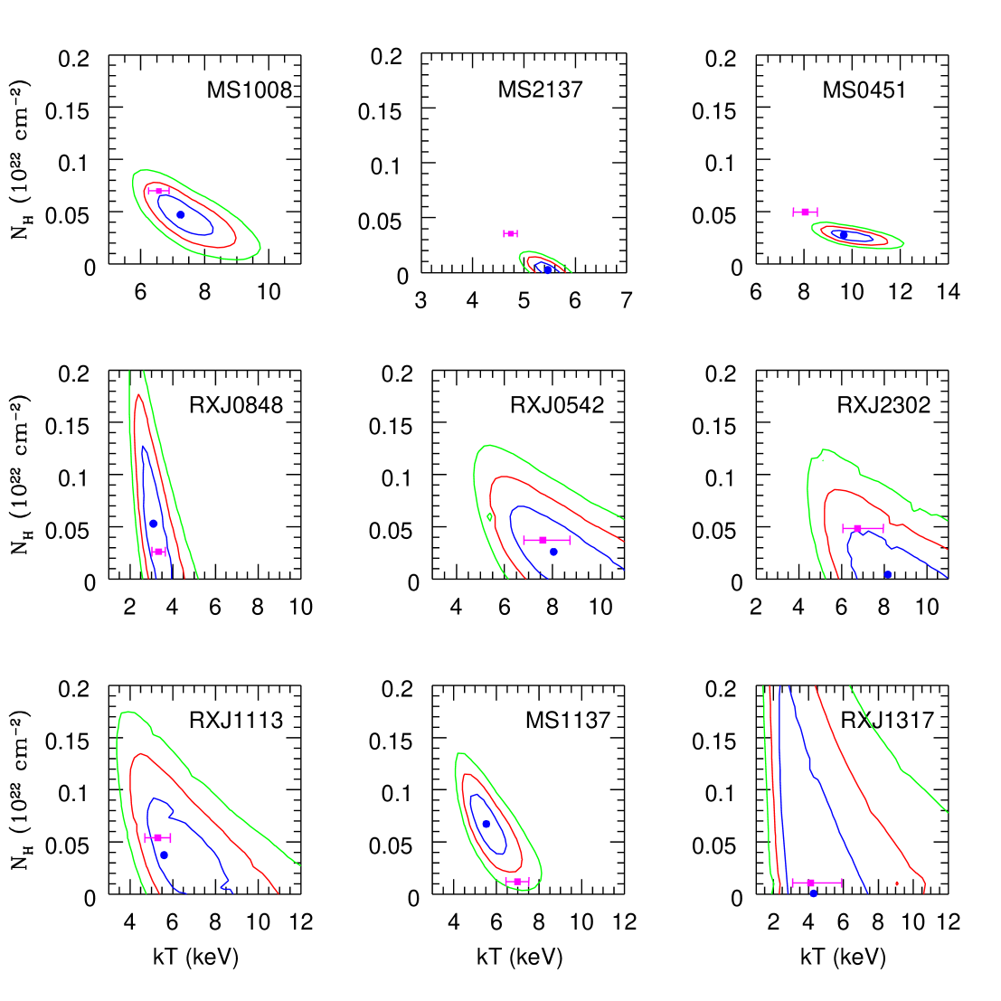
Figure 11: The plots show the 1–2–3 $\sigma$ confidence contours for the local column density $N_{H}$ and the temperature $kT$ for the first nine clusters observed with Chandra. The filled circle is the best–fit, and the filled square with $1\sigma$ error bars is best–fit point obtained fixing $N_{H}$ to the Galactic value.

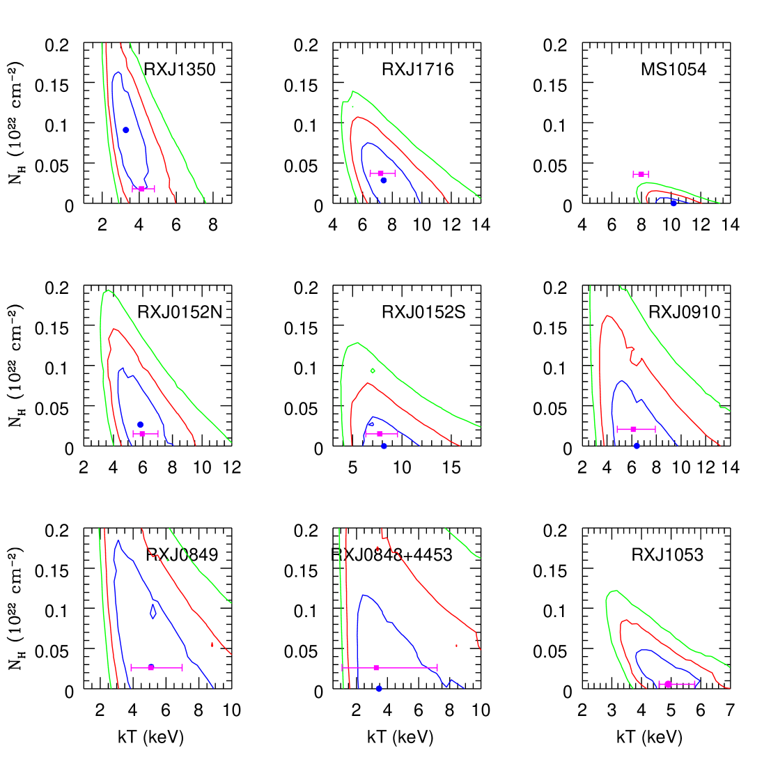
Figure 12: Same as 11 for the 8 highest z clusters observed with Chandra. The last panel (RXJ1053) refers to XMM only data.

In this Appendix, we briefly discuss the spectral analysis performed for each source of our sample, in order of increasing redshift. In Figures 7, 8 and 9, we show the background–subtracted spectra, along with the best–fit folded model, of the clusters observed with Chandra. In Figure 10 we show the spectra from the XMM data. In Figures 11 and 12 we also show the $kT$–$N_{H}$ confidence contours obtained when the Galactic absorption is left free, and compare the best-fit values with that obtained freezing $N_{H}$ to the Galactic value (see discussion in §3).

MS1008.1$-$1224

This cluster is part of the Extended Medium Sensitivity Survey sample (EMSS, Gioia et al. 1990). A detailed study of the mass of this system as derived from Chandra data and weak lensing analysis is presented in Ettori & Lombardi (2003). For our spectral analysis we used an extraction radius of maximum S/N of 108 arc sec, corresponding to 337 $h^{-1}$ kpc for the adopted $\Lambda$CDM cosmology, which includes $\simeq 9200$ net counts in the 0.3–10 keV band. Due to the relatively low redshift ($z=0.306$), emission lines of several elements are clearly visible in the spectrum around 2 and 5 keV (observed frame). The best–fit temperature is $kT=6.57\pm 0.32$ keV, in agreement with the previous ASCA measurement of $kT=7.3^{+2.4}_{-1.5}$ keV (Mushotzky & Scharf 1997) and of $7.2^{+1.0}_{-0.8}$ keV for the total emission found by Ettori & Lombardi (2003). We do not detect a gradient in the projected temperature in three annuli out to 100 arc sec. MS1008 was considered a prototype of a relaxed cluster, however in a recent optical study Athreya et al. (2002) found evidence of substructures, possibly indicating non–equilibrium in the gas, at least in the inner regions. The best–fit metallicity is $Z=0.24\pm 0.06Z_{\odot}$.

MS2137.3$-$2353

This very luminous EMSS cluster, at redshift $z=0.313$, was observed for 43 ks with ACIS–S in VFAINT mode, however the effective exposure was reduced to 33 ks in our analysis, mostly due to a large flare. The extraction radius of maximum S/N is 79 arc sec, corresponding to 250$h^{-1}$ kpc. Inside this circular region we found $\simeq 32000$ net counts in the 0.3–10 keV band. Due to the high count–rate in the center of the source, the VFAINT reduction results in the loss of some source photons. We repeated the analysis without the VFAINT cleaning procedure and found that the spectral fit is not affected (see also http://cxc.harvard.edu/cal/Acis/Cal_prods/vfbkgrnd/index.html#tth_sEc4). The best–fit temperature is $kT=4.75^{+0.10}_{-0.15}$ keV, in agreement with the ASCA result, $kT=4.4\pm 0.40$ keV (Mushotzky & Scharf 1997). There is a negative temperature gradient towards the inner regions. The temperature in the center is about 3.5 keV, whereas it is slightly below 6 keV at 30 arc sec, and it decreases below 4 keV in the outer regions. Very tight confidence intervals are obtained for the metallicity: $Z=0.33\pm 0.03\,Z_{\odot}$. This value is consistent, within 1 $\sigma$, with the ASCA result of $Z=0.41\pm 0.12\,Z_{\odot}$ as reported in Mushotzky and Loewenstein (1997).

MS0451.6$-$0305

This is the most luminous cluster in the EMSS sample. We measured $\simeq 3400$ net counts from an exposure with ACIS–I (14 ks), and $\simeq 17000$ net counts from an exposure with ACIS–S (42 ks) in the 0.3–10 keV band, inside an aperture of 98 arc sec radius. The best–fit temperature from the combined fit of the two spectra is $kT=8.05^{+0.50}_{-0.40}$ keV, in agreement with Vikhlinin et al. (2002) but lower than the ASCA measure of $kT=10.2^{+1.5}_{-1.3}$ keV (Mushotzky & Scharf 1997). This difference can be ascribed to a temperature gradient. In the Chandra data, the best–fit temperature ranges from 9 keV in the central 30 arc sec, to 7 keV at radii larger than 100 arc sec. The best–fit metallicity is $Z=0.32^{+0.07}_{-0.04}\,Z_{\odot}$. This value is different from the previous result from ASCA of $Z=0.15\pm 0.11\,Z_{\odot}$ (Donahue 1996). Our analysis of the inner 30 arc sec still gives a quite large metallicity, $Z=0.60\pm 0.15Z_{\odot}$, for a $kT\sim 9$ keV temperature. We argue that such a difference can be ascribed to the details of the analysis of the ASCA data, since a similar discrepance is found for MS1054 (see below).

RXJ0848+4456

This cluster, drawn from the ROSAT Deep Cluster Survey (RDCS, Rosati et al. 1998), is part of a deep observation (184.5 ks of effective exposure with ACIS–I) of the Lynx field. Its X–ray and optical properties and the discovery of a foreground group are discussed in detail in Holden et al. (2001). The spectral analysis presents some difficulties due to a colder, infalling group (RXJ0849+4455) along the line of sight, at a redshift $z=0.543$, slightly lower than the redshift of the main cluster, $z=0.570$. Despite the low number of net counts detected in the 0.3–10 keV band (850 for the cluster, within a 30 arc sec circle) the temperature is well constrained since the cutoff of the thermal spectrum falls just around 2 keV, near the peak of the efficiency curve of Chandra. We obtain $kT=3.24\pm 0.30$ keV (in close agreement with Holden et al. (2001) who followed a slightly different procedure), and a metallicity of $Z=0.51^{+0.22}_{-0.17}\,Z_{\odot}$. We also attempted to derive the metallicity of the colder group. We have only 200 net counts from a region of 37.4 arc sec radius. The temperature is well constrained ($kT=2.7^{+1.0}_{-0.6}$ keV), whereas for the metallicity we obtain only a large upper limit of $Z<0.6\,Z_{\odot}$ (1 $\sigma$ upper limit). Due to possible contamination from the brighter cluster, we do not include the colder group in our analysis.

RXJ0542.8$-$4100

This is a cluster from the RDCS sample at $z=0.634$. We collected 2200 net counts in the 0.3–10 keV band, within an aperture of 79 arc sec radius. The best–fit temperature is $kT=7.6^{+1.1}_{-0.8}$ keV for a metallicity of $Z=0.11_{-0.11}^{+0.13}\,Z_{\odot}$. We do not find evidence of a temperature gradient, although the surface brightness distribution shows a clear envelope, indicative a “cold front”. A detailed study of this cluster will be presented in Scharf et al. (in preparation).

RXJ2302.8+0844

This cluster was discovered in the RDCS at $z=0.734$. The 110 ks exposure reduces to an effective time of 108 ks after the standard reduction. We detect about 1450 net counts in the 0.3–10 keV band within a 49 arc sec circle. The best–fit temperature is $kT=6.7^{+1.3}_{-0.7}$ keV, for a metallicity of $Z=0.15_{-0.15}^{+0.14}\,Z_{\odot}$. The elongated morphology and the possible evidence for a central double peak suggest that the cluster may not be in a fully relaxed state.

RXJ1113.1$-$2615

This cluster was discovered in the WARPS survey (Perlman et al. 2002, Maughan et al. 2003). We detected $\sim\!1200$ net counts in the 0.3–10 keV band from a $39.4$ arc sec radius circular region. The high redshift ($z=0.73$), combined with the intermediate temperature, allowed us to determine the temperature with a 10% error, $kT=5.7^{+0.8}_{-0.7}$ keV. Also the metallicity is well constrained at a relatively high value, $Z=0.40\pm 0.18\,Z_{\odot}$. Our results are consistent, within the errors, with the analysis of Maughan et al. (2003).

MS1137.5+6625

This is the second most distant cluster in the EMSS survey. We detected $\sim 4200$ net counts in the 0.3–10 keV band from a circular region with a radius of 49 arc sec. For a redshift of $z=0.782$, we find a temperature of $kT=7.0\pm 0.5$ keV and a metallicity of $Z=0.21\pm 0.10\,Z_{\odot}$. The best–fit temperature is consistent with the value of $kT=6.3\pm 0.4$ keV found by Vikhlinin et al. (2002). We find a possible drop in the projected temperature to $\sim 6$ keV in the outer 30–100 arc sec, with low statistical significance.

RXJ1317.4+2911

The first analysis of this RDCS cluster was presented by Holden et al. (2002), along with its optical properties. The 115 ks exposure reduced to 110.5 ks after the reduction procedure. We detected about 230 net counts (in the 0.3–10 keV band) from a circular region with a radius of 29.5 arc sec, after the removal of pointsources. The best–fit temperature is $kT=4.0_{-0.8}^{+1.3}$ keV, for a metallicity of $Z=0.52_{-0.38}^{+0.60}\,Z_{\odot}$, this value is consistent with the Holden et al. (2002) analysis. It is, however, higher than that published by Vikhlinin et al. (2002) of $kT=2.2\pm 0.5$ keV. The discrepancy is significant at $2\sigma$. We argue that such a discrepancy can be ascribed to differences in the procedure of removing faint pointsources within the extraction region, which becomes critical for clusters with low S/N like this one. We notice also that the best–fit redshift from the X–ray analysis alone is $z\sim 1$, significantly different from the optically measured value of $z=0.805$.

RXJ1350.0+6007

The first Chandra analysis of this RDCS cluster, as well its optical study, was presented by Holden et al. (2002). We detected about 760 net counts in the 0.3–10 keV band from a circular region of 69 arc sec radius. The best–fit temperature is $kT=4.3_{-0.4}^{+1.3}$ keV, for a metallicity of $0.43_{-0.21}^{+0.44}\,Z_{\odot}$. These values are in close agreement with the Holden et al. (2002) analysis, and also in very good agreement with Vikhlinin et al. (2002) ($kT=4.3\pm 0.6$ keV). We found some evidence for a gradient in the projected temperature, from 3.5 to 5–6 keV going from the central 20 arc sec, to 20–40 and 40–100 arc sec annuli. A peculiar feature is that the metallicity is increasing for larger extraction radii (e.g. the metallicity rises by a factor of two when the redshift is left free). This is probably due to noise in the background spectrum, which becomes larger as the S/N decrease (see the discussion in Holden et al. 2002).

RXJ1716.9+6708

This cluster ($z=0.813$) was discovered in the NEP survey, and presented in Gioia et al. (1999). We use an effective Chandra exposure of 51 ks. We detected 1450 net counts in a region of 49.5 arc sec radius in the 0.3–10 keV band. The best–fit temperature is $kT=6.8_{-0.6}^{+1.1}$ keV, for a metallicity of $Z=0.49\pm 0.18\,Z_{\odot}$. These results are consistent, within 1$\sigma$, with the values reported by Gioia et al. (1999) using ASCA ($kT=5.7^{+1.4}_{-0.6}$ keV) and by Vikhlinin et al. (2002) ($kT=6.6\pm 0.8$ keV) using Chandra. We also find some hints of a higher projected temperature towards the center.

MS1054.5$-$0321

This is the most distant EMSS cluster, at $z=0.83$, subject to a large number of follow–up studies. The 90 ks Chandra exposure reduced to an effective exposure of 80 ks. We detected more than 10000 net counts in the 0.3–10 keV band from an aperture of 78 arc sec radius. The morphology shows clear evidences of substructures. We fit the region of higher S/N without separating the western, cooler clump, as in Jeltema et al. (2001). We detect a significant temperature gradient from $\sim 6$ keV in the inner 30 arc sec, to 8 keV in the outer 30–50, 50–80 arc sec rings. Our best–fit temperature is $kT=8.0\pm 0.5$ keV, for a metallicity of $0.24^{+0.07}_{-0.08}\,Z_{\odot}$. These results are in good agreement with those by Jeltema et al. (2001), considering that they analyzed the cooler clump separately, and by Vikhlinin et al. (2002). We disagree with the original ASCA result by Donahue et al. (1998), where the best–fit temperature was $12.3$ keV and the best–fit metallicity was much lower. This situation is similar to that of MS0451, thus indicating possible problems with the previous analysis of the ASCA data.

RXJ0152.7$-$1357

This cluster was reported in the RDCS (Della Ceca et al. 2002), in the WARPS (Ebeling et al. 2000) and SHARC (Romer et al. 2000) surveys. The system is a typical example of two major mass clumps in the process of merging, both at redshift $z=0.83$ (Demarco et al., in preparation). The same morphology is also well traced by the distribution of cluster galaxies. An independent detailed analysis of the Chandra data was recently presented by Maughan et al. (2003). We independently analyzed the two clumps which are well separated in the Chandra image.

For the northern clump we detected $\sim\!830$ net counts in the 0.3–10 keV band, in a circular region with a radius 58 arc sec. The best–fit temperature is $kT=5.9_{-0.7}^{+1.4}$ keV for a metallicity of $Z=0.13_{-0.13}^{+0.17}\,Z_{\odot}$. This result is in excellent agreement with that derived from global analysis of Beppo–SAX data by Della Ceca et al. (2000), as well as with that by Vikhlinin et al. (2002).

For the southern clump we detected $\sim\!570$ net counts in the 0.3–10 keV band, in a circular region with a radius 53 arc sec. The southern clump has a best–fit temperature of $kT=7.6_{-1.0}^{+2.5}$ keV with an upper bound on the metallicity of $Z<0.19\,Z_{\odot}$. This temperature is consistent within $1\sigma$ with the temperature of the northern clump. We notice that if the redshift is left free, we find for the southern clump a best–fit redshift $z=0.75$ (still within $1\sigma$ from the optical redshift $z=0.83$) and a temperature of $kT\sim 7.4$ keV, but a metallicity jumps to $Z\simeq 0.6\,Z_{\odot}$, much higher than that of the northern clump. Our temperatures are in good agreement with that of Maughan et al. (2003) as well as with the analysis of Huo et al. (2003).

RXJ0910+5422

This is one of the four RDCS clusters at $z>1$ ($z=1.106$). Its discovery as well as the first analysis of the Chandra data was presented in Stanford et al. (2002). It was observed in two pointings for a total of 173 ks, resulting in an effective exposure of 170 ks. We detect $\sim\!430$ net counts in the 0.3–10 keV band from a region of 25 arc sec. The best–fit temperature is $kT=6.6_{-1.4}^{+2.0}$ keV. We obtain only an upper bound for the metallicity $Z<0.25\,Z_{\odot}$. These values are in good agreement with the previous analysis by Stanford et al. (2002).

RXJ0849+4452 and RXJ0848+4453

These two systems, part of the RDCS sample, are likely part of a super–structure at $z\simeq 1.26$ (Rosati et al. 1999). They were the target of a long Chandra exposure (the Lynx field, with an effective exposure of 184.5 ks). A detailed analysis of the Chandra observations was presented in Stanford et al. (2001). At present, these are the two highest redshift clusters selected and analyzed in X–rays.

RX0849+4452 shows a relaxed morphology, possibly in an evolved dynamical stage. For RX0849+4452 we detect 360 net counts in the 0.3–10 keV band from a circular region of 23.6 arc sec radius in the Chandra exposure. The best–fit temperature is $kT=5.2_{-1.1}^{+1.7}$ keV, with an upper bound on the metallicity of $Z<0.5\,Z_{\odot}$. This result is in excellent agreement with the previous analysis by Stanford et al. (2002), which gives $kT=5.8^{+2.8}_{-1.7}$ keV for a fixed metallicity of $Z=0.3\,Z_{\odot}$. We detect also $\sim 630$ net counts from the XMM exposure (EPIC–PN + MOS detectors). The analysis of the XMM data for this cluster yields $kT=6.6\pm 1.1$ keV. We obtain only a $1\sigma$ upper bound for the metallicity of $Z<0.38\,Z_{\odot}$. These results are in agreement with the Chandra data within the errors. The combined analysis (Chandra + XMM), gives $kT=5.6_{-0.6}^{+0.8}$ keV, with a metallicity of $Z=0.09_{-0.07}^{+0.24}\,Z_{\odot}$a . In our analysis we use the results from the combined fit Chandra + XMM.

As for RXJ0848+4453, we detected $\sim\!130$ net counts in the 0.3–10 keV band in a region of 19.7 arc sec radius. The best–fit temperature is $kT=3.3_{-1.0}^{+2.5}$ keV. We obtain a very large $1\sigma$ upper bound for the metallicity $Z<1.3\,Z_{\odot}$. This temperature is higher than that derived in the previous analysis by Stanford et al. (2002) ($kT=1.6^{+0.8}_{-0.6}$ keV), but still consistent within less than 2$\sigma$ due to large error bars. Unfortunately, the XMM data for this cluster are not useful due to the very low signal–to–noise. The difference in the best–fit temperature is in mostly due to the different extraction radius used: 20” as opposed to the 35” in Stanford et al. (2001). By repeating the analysis with a radius of 35”, we found $kT=2.4_{-0.8}^{+1.2}$ keV, thus in agreement with Stanford et al. (2001).

RXJ1053+5735

For this target we used only XMM data from the 100 ks VP observation of the Lockman Hole (Hashimoto et al. 2002). The analysis of clearly shows two clumps. For the eastern clump we detected about 430 net counts in the 0.5–8 keV band for the PN camera, and 280 net counts in the 0.5–8 keV band for the two MOS cameras, in an elliptical region with semi–axis of 32 and 30.4 arc sec. The best–fit temperature is $kT=3.2\pm 0.4$ keV for a metallicity of $Z=0.60_{-0.22}^{+0.60}\,Z_{\odot}$. For the western clump, we detected about 530 net counts in the 0.5–8 keV band for the PN camera, and 340 net counts in the 0.5–8 keV band for the two MOS cameras, in an elliptical region with semi–axis of 27.2 and 28.8 arc sec. The best–fit temperature is $kT=5.8_{-0.7}^{+1.2}$ keV for a metallicity of $Z=0.40^{+0.21}_{-0.14}\,Z_{\odot}$. These values are consistent with those found by Hashimoto et al. (2002), considering that they assumed $z=1.26$ (Thompson et al. 2001) instead of the revised $z=1.15$ (Hasinger 2003, private communication).

We also present the result of the fit of the total cluster spectrum. We obtain a best–fit temperature of $kT=4.9_{-0.3}^{+0.9}$ keV for a metallicity of $Z=0.39_{-0.10}^{+0.14}\,Z_{\odot}$. The metallicity is $Z>0.10Z_{\odot}$ at the 90% c.l., thus constituting the only detection of the Fe line at a significant confidence level at $z>1$ in our current sample.

Table 1: Chandra Observations

Cluster	z	Obs ID	Exposure	Detectors and obs. mode	$R_{ext}$”	Survey
MS1008.1$-$1224	0.306	926	44	ACIS–I; VFAINT	108.0	EMSS
MS2137.3$-$2353	0.313	928	33	ACIS–S; VFAINT	79.0	EMSS
MS0451.6$-$0305	0.539	529+902	14+42	ACIS–I/S; VFAINT	98.0	EMSS
RXJ0848+4456	0.570	1708+927	184.5	ACIS–I; VFAINT	30.0	RDCS
RXJ0542.8$-$4100	0.634	914	50	ACIS–I; FAINT	78.7	RDCS
RXJ2302.8+0844	0.734	918	108	ACIS–I; FAINT	49.0	RDCS
RXJ1113.1$-$2615	0.730	915	103	ACIS–I; FAINT	39.4	WARPS
MS1137.5+6625	0.782	536	117	ACIS–I; VFAINT	49.2	EMSS
RXJ1317.4+2911	0.805	2228	110.5	ACIS–I; VFAINT	39.4	RDCS
RXJ1350.0+6007	0.810	2229	58	ACIS–I; VFAINT	68.9	RDCS
RXJ1716.9+6708	0.813	548	51	ACIS–I; FAINT	59.0	NEP
MS1054.5$-$0321	0.832	512	80	ACIS–S; FAINT	78.7	EMSS
RXJ0152.7$-$1357N	0.835	913	36	ACIS–I; FAINT	58.0	RDCS/WARPS/SHARCS
RXJ0152.7$-$1357S	0.828	913	36	ACIS–I; FAINT	52.7	RDCS/WARPS/SHARCS
RXJ0910+5422	1.106	2452+2227	170	ACIS–I; VFAINT	24.6	RDCS
RXJ0849+4452	1.261	1708+927	184.5	ACIS–I; VFAINT	29.5	RDCS
RXJ0848+4453	1.273	1708+927	184.5	ACIS–I; VFAINT	29.5	RDCS

Note. — The sample of 17 clusters observed with Chandra. The 3rd columns is the ID of the exposure in the Chandra Archive. The 4th column refers to the effective exposure time in ks, after removal of high background intervals. The extraction radius $R_{ext}$ is given in arc seconds.

Table 2: XMM Observations

Cluster	z	exposure	detector	$R_{ext}$”	survey
RXJ1053+5735	1.15	94.5	PN + 2 MOS	32	Lockman Hole
RXJ0849+4452	1.26	112.0	PN + 2 MOS	29.5	RDCS

Note. — The two XMM observations considered in this Paper. The 3rd column refers to the effective exposure time in ks, after removal of high background intervals. The 4th column shows the detectors used. The extraction radius $R_{ext}$ is given in arc seconds.

Table 3: Spectral fits from Chandra and XMM observations

Cluster	kT (keV)	$Z/Z_{\odot}$	$N_{H}$ (cm-2)
MS1008.1$-$1224	$6.57\pm 0.32$	$0.24\pm 0.06$	$7.26\times 10^{20}$
MS2137.3$-$2353	$4.75^{+0.10}_{-0.15}$	$0.33\pm 0.03$	$3.55\times 10^{20}$
MS0451.6$-$0305	$8.05^{+0.50}_{-0.40}$	$0.32^{+0.07}_{-0.04}$	$5.00\times 10^{20}$
RXJ0848+4456	$3.24\pm 0.30$	$0.51^{+0.22}_{-0.17}$	$2.63\times 10^{20}$
RXJ0542.8$-$4100	$7.6^{+1.1}_{-0.8}$	$0.11_{-0.11}^{+0.13}$	$3.73\times 10^{20}$
RXJ2302.8+0844	$6.7_{-0.7}^{+1.3}$	$0.15_{-0.15}^{+0.14}$	$4.85\times 10^{20}$
RXJ1113.1$-$2615	$5.7^{+0.8}_{-0.7}$	$0.40\pm 0.18$	$5.50\times 10^{20}$
MS1137.5+6625	$7.0\pm 0.5$	$0.21^{+0.10}_{-0.11}$	$1.21\times 10^{20}$
RXJ1317.4+2911	$4.0_{-0.8}^{+1.3}$	$0.52_{-0.38}^{+0.60}$	$1.10\times 10^{20}$
RXJ1350.0+6007	$4.3_{-0.4}^{+1.3}$	$0.43_{-0.21}^{+0.44}$	$1.80\times 10^{20}$
RXJ1716.9+6708	$6.8_{-0.6}^{+1.1}$	$0.49\pm 0.18$	$3.72\times 10^{20}$
MS1054.5$-$0321	$8.0\pm 0.5$	$0.24_{-0.08}^{+0.07}$	$3.61\times 10^{20}$
RXJ0152.7$-$1357N	$5.9_{-0.7}^{+1.4}$	$0.13_{-0.13}^{+0.17}$	$1.54\times 10^{20}$
RXJ0152.7$-$1357S	$7.6_{-1.0}^{+2.5}$	$<0.19$	$1.54\times 10^{20}$
RXJ0910+5422	$6.6_{-1.4}^{+2.0}$	$<0.25$	$2.10\times 10^{20}$
RXJ0849+4452	$5.6_{-0.6}^{+0.8}$	$0.09^{+0.24}_{-0.07}$	$2.63\times 10^{20}$
RXJ0848+4453	$3.3_{-1.0}^{+2.5}$	$0.25_{-0.25}^{+0.95}$	$2.63\times 10^{20}$
RXJ1053+5735	$4.9_{-0.3}^{+0.9}$	$0.39_{-0.10}^{+0.14}$	$5.7\times 10^{19}$
RXJ1053+5735 EAST	$3.2\pm 0.4$	$0.60^{+0.60}_{-0.22}$	$5.7\times 10^{19}$
RXJ1053+5735 WEST	$5.8_{-0.7}^{+1.2}$	$0.40_{-0.14}^{+0.21}$	$5.7\times 10^{19}$

Note. — Results from the spectral fits with the TBABS$\times$MEKAL model. The local column density is always frozen at the galactic value, measured by Dickey & Lockman (1990) and shown in the 4th column. Error bars refer to $1\sigma$ confidence level.

Table 4: Average Iron Abundance from combined fits

$\langle z\rangle$	$Z/Z_{\odot}$ ($kT>5$ keV)	$Z/Z_{\odot}$ ($kT<5$ keV)
0.30	$0.30^{+0.03}_{-0.2}$ [2]	–
0.58	$0.29^{+0.07}_{-0.03}$ [2]	$0.51^{+0.22}_{-0.17}$ [1]
0.80	$0.25^{+0.04}_{-0.06}$ [7]	$0.50^{+0.29}_{-0.22}$ [2]
1.20	$0.22^{+0.12}_{-0.10}$ [3]	$0.65^{+0.50}_{-0.30}$ [2]

Note. — The first comlumn shows the average redshift of the bin. The number of the clusters of each combined fit is shown in parenthesis.

Figure 6: Distribution of the best–fit metallicity values from the combined fit of the 4 clusters in our sample at $z>1$, when simulated $10^{3}$ times (solid line). The input metallicity is $0.3Z_{\odot}$. The dashed line is the result of the simulations when only the three clusters observed with Chandra are considered.

Figure 7: The spectra of the clusters observed with Chandra with the folded thermal best–fit model (continuous lines). The lower panels show the residuals. Clusters are sorted by increasing redshift. Note that in the case of MS0451 we show the data for ACIS–I and for ACIS–S.

Figure 8: The same as Figure 7.

Figure 9: The same as Figure 7.

Figure 10: The spectra of the clusters observed with XMM with the folded thermal best–fit model (continuous lines). The lower panels show the residuals. The three spectra for RXJ1053 refer to PN, MOS thick filter and MOS thin filter data while two spectra of RXJ0849 refer to PN and MOS data. We also show spectra and best fits for the eastern and western clumps of RXJ1053.

References

- (1) Allen, S.W., & Fabian, A.C. 1998, MNRAS, 297, L63
- (2) Anders, E., Grevesse, N. 1989, Geochimica et Cosmochimica Acta, 53, 197
- (3) Arnaud, K.A. 1996, “Astronomical Data Analysis Software and Systems V”, eds. Jacoby G. and Barnes J., ASP Conf. Series vol. 101, 17
- (4) Athreya, R.M., Mellier, Y., van Waerbecke, L., Pelló, R., Fort,, & Dantel–Fort, M. 2002, A&A, 384, 743
- (5) Babul, A., Balogh, M. L., Lewis, G. F., & Poole, G. B. 2002, MNRAS, 330, 329
- (6) Bialek, J. J., Evrard, A. E., & Mohr, J. J. 2001, ApJ, 555, 597
- (7) Boschin, W. 2002, A&A, 396, 397
- (8) Buote, D. A. 2000, ApJ, 539, 172
- (9) Davis, D. S., Mulchaey, J. S., & Mushotzky, R. F. 1999, ApJ, 511, 34
- (10) De Grandi, S., & Molendi, S. 2001, ApJ, 551, 153
- (11) Della Ceca, R., Scaramella, R., Gioia, I.M., Rosati, P., Fiore, F., & Squires, G. 2000, A&A, 353, 498
- (12) Dickey & Lockman, 1990, ARAA, 28, 215.
- (13) Donahue, M. 1996, ApJ, 468, 79
- (14) Donahue, M., Voit, G.M., Gioia, I., Luppino, G., Hughes, J.P., & Stocke, J.T. 1998, ApJ, 502, 550
- (15) Dupke, R.A., White, R. 2000, ApJ, 537, 123
- (16) Ebeling, H., Jones, L.R., Perlman, E., Scharf, C., Horner, D., Wegner, G., Malkan, M., Fairley, B.W., & Mullis, C.R. 2000, ApJ, 534, 133
- (17) Ettori, S., Allen , S.W., & Fabian, A. C. 2001, MNRAS, 322, 187
- (18) Ettori S., Fabian A.C., Allen S.W., Johnstone R.M. 2002, MNRAS, 331, 635
- (19) Ettori, S., & Lombardi, M. 2003, A&A, in press (astro-ph/0212167)
- (20) Ettori, S., Tozzi, P., & Rosati, P. 2003, A&A, 398, 879
- (21) Finoguenov, A., David, L. P., & Ponman, T. J. 2000, ApJ, 544, 188
- (22) Finoguenov, A., Arnaud, M., & David, L.P. 2001, ApJ, 555, 191
- (23) Finoguenov, A., Jones, C., Boehringer, H., Ponman, T.J. 2002, ApJ, 578, 74
- (24) Fukazawa, Y., Makishima, K., Tamura, T., Ezawa, H., Xu, H., Ikebe, Y., Kikuchi, K., Ohashi, T. 1998, PASJ, 50, 187
- (25) Gastaldello, F., & Molendi, S. 2002, ApJ, 572, 160
- (26) Gioia, I.M., Henry, J.P.,Maccacaro, T., Morris, S.L., & Stocke, J.T. 1990, ApJ, 356, L35
- (27) Gioia, I.M., Henry, J.P., Mullis, C.R., Ebeling, H., & Wolter, A. 1999, AJ, 117, 2608
- (28) Grevesse, N., & Sauval, A.J. 1998, Space Science Reviews, 85, 161
- (29) Hasinger, G., Altieri, B., Arnaud, M., et al. 2001, A&A, 365, L45
- (30) Hashimoto, Y., Hasinger, G., Arnaud, M., Rosati, P., Miyaji, T. 2002, A&A, 381, 841
- (31) Holden, B.P., Stanford, S.A., Rosati, P., Squires, G., Tozzi, P., Fosbury, R.A.E., Papovich, C., Eisenhardt, P., Elston, R., & Spinrad, H. 2001, AJ, 122, 629
- (32) Holden, B.P., Stanford, S.A., Squires, G.K., Rosati, P., Tozzi, P., Eisenhardt, P., & Spinrad, H. 2002, AJ, 124, 33
- (33) Huo, Z., Xue, S., Xu, H., Squires, G., & Rosati, P. 2003, submitted
- (34) Jansen, F., Lumb, D., Altieri, B., et al. 2001, A&A, 365, L1
- (35) Jeltema, T.E., Canizares, C.R., Bautz, M.W., Malm, M.R. Dobahue, M., Garmire, G.P. 2001, ApJ, 562, 124
- (36) Kaastra, J.S. 1992, “An X–ray Spectral Code for Optically Thin Plasmas” (Internal SRON–Leiden Report, updated version 2.0)
- (37) Lewis, A.D., Ellingson, E., Morris, S.L., & Carlberg, R.G. 1999, ApJ, 517, 587
- (38) Lewis, A.D., Buote, D. A., & Stocke, J.T. 2003, ApJ in press, astro-ph/0209205
- (39) Liedahl, D.A., Osterheld, A.L., Goldstein, W.H. 1995, ApJ, 438, L115
- (40) Mainieri, V., Bergeron, J., Hasinger, G., Lehmann, I., Rosati, P., Schmidt, M., Szokoly, G., & Della Ceca, R. 2002, A&A, 393, 425
- (41) Markevitch, M., & Vikhlinin, A. 2001, ApJ, 563, 95
- (42) Matsumoto, H., Tsuru, T.G., Fukazawa, Y., Hattori, M., & Davis, D.S. 2000, PASJ, 52, 153
- (43) Matsushita, K., Belsole, E., Finoguenov, A., B hringer, H. 2002, A&A, 386, 77
- (44) Maughan, B.J., Jones, L.R., Ebeling, H., Perlman, E., Rosati, P., & Frye, C. 2003, submitted, astro-ph/0301218
- (45) Mushotzky, R.F., & Loewenstein, M. 1997, ApJ, 481, L63
- (46) Mushotzky, R.F., & Scharf, C.A. 1997, ApJ, 482, L13
- (47) Nousek, J.A., & Shue, D.R. 1989, ApJ, 342, 1207
- (48) Perlman E.S. et al. 2002, ApJ Suppl., 140, 265
- (49) Pipino, A., Matteucci, F., Borgani, S., Biviano, A., 2002, NewA, 7, 227
- (50) Ponman, T.J., Cannon, D.B., Navarro, J.F. 1999, Nature, 397, 135
- (51) Renzini, A. 1997, ApJ, 488, 35
- (52) Romer, A.K., Nichol, R.C., Holden, B.P., Ulmer, M.P., Pildis, R.A., Merrelli, A.J., Adami, C., Burke, D.J., Collins, C.A., Metevier, A.J., Kron, R.G., & Commons, K. 2000, ApJS, 126, 209
- (53) Rosati, P., Della Ceca, R., Burg, R., Norman, C., Giacconi, R. 1998, ApJ, 492, L21
- (54) Rosati, P, Stanford, S.A., Eisenhardt, P.R., Elston, R., Spinrad, H., et al. 1999. AJ, 118
- (55) Rosati, P., Borgani, S., & Norman, C. 2002, ARAA, 40, 539
- (56) Stanford, S.A., Holden, B.P., Rosati, P., Tozzi, P., Borgani, S., Eisenhardt, P.R., & Spinrad, H. 2001, ApJ, 552, 504
- (57) Stanford, S.A., Holden, B.P., Rosati, P., Eisenhardt, P.R., Stern , D., Squires, G., & Spinrad, H. 2002, AJ, 123, 619
- (58) Tamura, T., Bleeker, J. A. M., Kaastra, J. S., Ferrigno, C., & Molendi, S. 2001, A&A, 379, 107
- (59) Thompson et al. 2001, A&A, 377, 778
- (60) Tornatore, L., Borgani, S., Springel, V., Matteucci, F., Menci, N., & Murante, G. 2003, MNRAS, submitted
- (61) Tozzi, P. & Norman, C. 2001, ApJ, 546, 63
- (62) Vikhlinin, A., VanSpeybroek, L., Markevitch, M., Forman, W.R., & Grego, L. 2002, ApJL, 578, 107
- (63) Voit, G.M., Bryan, G.L., Balogh, M.L., Bower, R.G. 2002 ApJ, 576, 601
- (64) White, D. A. 2000, MNRAS, 312, 663
- (65) Wilms, J., Allen, A., & McCray, R. 2000, ApJ, 542, 914