The three dimensional power spectrum of dark and luminous matter from the VIRMOS-DESCART cosmic shear survey

Abstract

We present the first optimal power spectrum estimation and three dimensional deprojections for the dark and luminous matter and their cross correlations. The results are obtained using a new optimal fast estimator (Pen, 2003), deprojected using minimum variance and SVD techniques. We show the resulting 3-D power spectra for dark matter and galaxies, and their covariance for the VIRMOS-DESCART weak lensing shear and galaxy data. The survey is most sensitive to nonlinear scales $k_{\rm NL}\sim 1h$Mpc^-1. On these scales, our 3-D power spectrum of dark matter is in good agreement with the RCS 3-D power spectrum found by Tegmark & Zaldarriaga (2002). Our galaxy power is similar to that found by the 2MASS survey, and larger than that of SDSS, APM and RCS, consistent with the expected difference in galaxy population.

We find an average bias $b=1.24\pm 0.18$ for the $I$ selected galaxies, and a cross correlation coefficient $r=0.75\pm 0.23$. Together with the power spectra, these results optimally encode the entire two point information about dark matter and galaxies, including galaxy-galaxy lensing. We address some of the implications regarding galaxy halos and mass-to-light ratios. The best fit “halo” parameter $h\equiv r/b=0.57\pm 0.16$, suggesting that dynamical masses estimated using galaxies systematically underestimate total mass.

Ongoing surveys, such as the Canada-France-Hawaii-Telescope-Legacy survey will significantly improve on the dynamic range, and future photometric redshift catalogs will allow tomography along the same principles.

1 Introduction

The recent measurements of the cosmic microwave background anisotropies have moved physical cosmology into a new era of precision measurements (Spergel et al., 2003). The cosmic microwave background perturbations can be cleanly computed from first principles, and have been measured with high accuracy. This allows a clean inference of conditions at the redshift of recombination, $z\sim 1089$. To complete the picture, a separate measurement of the state of the universe at lower redshifts is required. The original WMAP results used the distribution of optical galaxies as a proxy for the distribution of total matter. The dominant uncertainty in such an exercise is the relationship between galaxies and total mass (Contaldi et al., 2003).

A direct measure of the dynamics of total mass is clearly desirable, as well as a quantitative measure of the relationship between total mass and visible matter. Statistical weak gravitational lensing provides such a handle, and direct measurements are already providing accuracies on cosmological parameters such as $\sigma_{8}$ comparable to indirect galaxy techniques (Bacon et al., 2002; Refregier et al., 2002; Hoekstra et al., 2002; Van Waerbeke et al., 2002; Jarvis et al., 2002; Brown et al., 2002; Hamana et al., 2002).

The gravitational field from the inhomogeneity of the dark matter distribution disturbs the light from background galaxies and distorts the apparent images of galaxies. When this distortion is small, it is called the weak gravitational lensing. Since gravity acts equally on all particles, gravitational lensing is a complete probe of the total matter distribution. Gravity is dominated by dark matter, which does not involve complicated gas physics, which makes gravitational lensing relatively straightforward to calculate from analytical models and N-body simulations (White & Hu, 2000). All these advantages make weak gravitational lensing a powerful probe of cosmological parameters and the matter distribution.

So far all analyses of weak lensing data have been parametric by comparing the observed two dimensional correlations of shear to the predictions of standard models. A direct optimal statistical analyses of the data sets has so far been beyond the scope of computational resources. Pen et al. (2002) presented the first angular power spectra obtained from inversions of the correlations functions. Brown et al. (2002) did maximum likelihood estimation on a low signal-to-noise data set.

In this paper, we extract the 3-D dark and luminous matter power spectrum from the 2-D weak lensing measurements in the VIRMOS-DESCART survey. Similar works have been tested successfully in inverting the 2-D galaxy angular correlations to 3-D galaxy power spectrum (Maddox et al., 1990; Baugh & Efstathiou, 1993; Dodelson & Gaztañaga, 2000; Eisenstein & Zaldarriaga, 2001; Dodelson et al., 2002; Maller et al., 2003). By measuring the distribution of galaxies and dark matter from the same survey, we find a direct measure of the cross correlation (Hoekstra et al., 2002).

2 Data

The VIRMOS-DESCART data consist of four uncorrelated patches (referred as fields F02, F10, F14 and F22 according to their RA position) of about 4 square-degrees each and separated by more than 40 degrees. The fields have been observed with the CFH12k panoramic CCD camera, mounted at the Canada-France-Hawaii Telescope prime focus, over the periods between January 1999 and November 2001. The observations and data reduction have been described in previous VIRMOS-DESCART cosmic shear papers (Van Waerbeke et al., 2000; Van Waerbeke et al., 2001; Van Waerbeke et al., 2002).

The observations have been done with the I-band filter available on the CFH12k camera a with typical exposure time of one hour. The final cosmic shear catalog contains 392,055 galaxies with magnitude $I_{AB}>22$ and median $I_{AB}=$23.6. Several careful checks have demonstrated that systematic residuals are very small. However, Van Waerbeke et al. (2001); Van Waerbeke et al. (2002) and Pen et al. (2002) have shown that a B-mode signal still remains on scales larger than 10 arc-minutes. Its origin is not yet understood.

The redshift distribution was modeled by the procedure described in Van Waerbeke et al. (2001) using the photometric redshifts from the Hubble deep fields (HDF). Here we performed the same analyses for all the galaxies with magnitude $I_{AB}>22$. The resulting histogram for this sample with their appropriate noise weights is shown in Figure 1. It was modelled from the photometric redshifts of the Hubble Deep Fields north and South (see Van Waerbeke et al. (2001)). In the absence of any spectroscopic survey deeper than $I_{AB}=22$ this is the best redshift estimate at the moment.

Figure 1: The top histogram shows the source weighted redshift distribution of the faint $I_{AB}>22$ catalog modeled from the HDF. The bottom histogram shows the bright $20<I_{AB}<21$ galaxy redshift distribution of the catalog modeled from the CFRS (see section 4), and the dotted curve is the fitting formula used in our analyses.

To compute the galaxy angular power spectra, the galaxy photometries were calibrated. A mask file was constructed on a grid spaced 6.18 arc seconds. For the lens plane sample, we chose a magnitude range $20<I_{AB}<21$, which contains 20657 galaxies.

3 2-D Power Spectrum Estimation

Given a reduced galaxy catalog, the first stage in the information compression process is to produce a two dimensional angular power spectrum, which encodes all two points information. Each galaxy has two observables: a position angle $\theta$ and axis ratio $e$, from which one forms the two polarization components $e_{1}=e\cos(2\theta)$ and $e_{2}=e\sin(2\theta)$. The data set contains close to a million degrees of freedom. A direct optimal power estimation requires ${\cal O}(N^{3})$ operations, which is completely intractable computationally. One could try to bin the data on a coarse grid to reduce the computational cost (White & Hu, 2000). Current processing power allows one to deploy about 50 grid cells on a side in such a treatment, corresponding to about 3 arc minute cells. Such a coarse binning unfortunately looses information. Karhunen-Loeve compression still involves an initially expensive eigenmode expansion, which is not tractible for a data set of this size.

We applied a novel fast matrix solver, which reduces the problem from ${\cal O}(N^{3})$ to ${\cal O}(N\log N)$ while still being optimal. (Pen, 2003). The galaxy catalog for each field is binned onto a square grid 1024 cells wide, and power is estimated directly on this grid. The power for the individual fields are then combined by the procedure of Wang et al. (2002). The Fisher matrix, error bars, and window functions are monte-carloed using 1000 realizations. The angular width of the grid was chosen to be 3.01 degrees, which is a little larger than the largest dimension of any field. For the lowest wave numbers along the longest direction of the grid this introduces an artificial aliasing due to periodic boundary conditions. In principle this could be avoided with a two level grid as described in Padmanabhan et al. (2002), but this has not yet been implemented on the multi-grid accelerated scheme. Since we do not use the lowest wave number bin in our analysis, this should not have a significant effect on our results. The analysis is based on a quadratic estimator with optimal weights relative to a model prior. We chose the parameters of the LCDM model in table 1. Several strategic choices are made in the process. The dark matter and galaxy power spectrum were estimated independently. To estimate the cross correlation, both must be taken into account simultaneously. When one allows for a prior correlation of dark matter with galaxies, the eigenmodes of the power are no longer dark matter and galaxy power, but linear sums and differences.

Model	$\Omega_{m}$	$\Omega_{\Lambda}$	$\sigma_{8}$	$\Gamma$	$h$
LCDM	0.27	0.73	0.9	0.19	0.71
SCDM1	1.0	0.0	0.5	0.19	0.71
SCDM2	1.0	0.0	0.5	0.7	0.71

Table 1: Cosmological models used to test the inversion.

The priors also gave equal E and B mode weights. The signal is known to have measurable B mode contamination (Pen et al., 2002), for whose separation a symmetric weight seemed most robust. Unequal priors lead to different window functions for the two modes, making comparisons tricky. A further potential complication is the additive white noise calibration in the power spectrum. As described in Pen et al. (2002), the intrinsic distribution of the unlensed ellipticity distribution can not be measured, so the two point shear correlation function at zero lag is completely unknown. This translates into an additive white noise factor in the power spectrum. Normally the noise is subtracted from the power spectrum estimator, and in our case, we estimate the noise by randomly rotating galaxies. This will cancel the correlation function at zero lag (which is invariant under rotations), and determine a fixed value of the integration constant. At large $l$ this can lead to a systematic underestimate of the power.

The reduced catalogues also have a statistical weight for each galaxy, which in Gaussian analyses is equal to the inverse noise variance. A random rotation would assign a noise equal to the observed ellipticity, but such a procedure biases the estimated power spectrum. Instead, the noise was assigned using the table lookup described by Van Waerbeke et al. (2000). Our power spectrum analysis thus has a different procedure for the noise and weights.

Figure 2 is the power spectrum of cosmic shear, which represents the fluctuations in the projected surface density

$$\kappa(\hat{\bf n})=\frac{\Sigma(\hat{\bf n})}{\Sigma_{cr}},$$ (1)

where

$$\Sigma_{cr}=\frac{c^{2}}{4\pi G}\frac{D_{s}}{D_{d}D_{ds}}.$$ (2)

$\Sigma(\hat{\bf n})$ is the surface density, $\hat{\bf n}$ is the direction on the sky. $D_{d}$, $D_{ds}$ and $D_{s}$ are the angular-diameter distance between the observer and lens, lens and source, observer and source respectively.

The dashed boxes indicate the E-type power-spectrum, while the crosses denote the B-type power. The solid boxes with error bars are the subtracted power $E-B$, which is the quantity we used to calculate the three dimensional power. For the difference powers, the error bars are calculated by the quadrature sum $\sqrt{{\sigma_{E}}^{2}+B^{2}}$. The $B$ mode is taken as a diagnostic for the error estimate, and we only added the value to the diagonal of the covariance matrix. Correlations between scales are not accounted for. The dashed straight line is the noise, which dominates at small angular scales. When noise dominates, the inverse noise weighted two point correlation function is an optimal estimator. The solid curve line is the power spectrum projected by the Limber equation from the three dimensional power using the code by Smith et al. (2002). We note that the errors are dominated by the $B$ mode, and eyeballing the plots, one could see up to three independent useful power spectrum measurements.

Figure 2: Spherical harmonic power spectrum. The dashed boxes indicate the raw E-type power-spectrum, while the crosses denote the B-type power. The solid boxes with error bars are $E-B$, which is the quantity we used to calculate the three dimensional power. Their error bars are the quadrature sum $\sqrt{{\sigma_{E}}^{2}+B^{2}}$. We have shifted the solid boxes with error bars to larger l slightly, in order to be distinguished with E-type and B-type power. The dashed straight line is the noise. The solid curved line is the model prediction for LCDM (see table 1).

To measure the distribution of luminous matter, we chose a magnitude range which traces the redshift distribution of lenses. The range $20<I_{AB}<21$ results in a differential redshift contribution shown in Figure 3, which is well matched to the lens weights. We used this magnitude range to measure the galaxy power spectrum shown in Figure 4.

Figure 3: The contribution to 2-D power spectrum by the 3-D power spectrum from different redshifts for a fixed angular scale $l=956$. The dotted line is for the galaxies. The solid line is for the dark matter.

Figure 4: The circles indicate the power spectrum for galaxies $20<I_{AB}<21$. The dashed line is the Poisson noise, and the solid line is the Limber equation prediction for luminous matter perfectly tracing dark matter. The dot-dashed and dotted lines are the projection of the best fit power spectra parametrized as $\Delta^{2}=(k/k_{0})^{n}$, for $n=1.7$ and $k_{0}=0.16(h\rm Mpc^{-1})$, as well as $n=1.8$ and $k_{0}=0.18(h\rm Mpc^{-1})$ respectively.

In the two dimensional projection, we fitted for a parametrized power spectrum $\Delta^{2}=(k/k_{0})^{n}$. This corresponds to a power law correlation function of the form $\xi=(r/r_{0})^{-n}$, with $r_{0}=2\left[\pi/2\sin(n\pi/2)\Gamma(2-n)\right]^{1/n}/k_{0}$. We used two values of $n$: 1.8 and 1.7. For $n=1.8$, the best fit correlation length is $k_{0}=0.22\pm 0.010h$Mpc^-1 for the $I$ selected galaxy population at weighted redshift $z_{m}=0.36$. The corresponding correlation length is $r_{0}=4.79\pm 0.22h^{-1}$ Mpc. The shallower slope $n=1.7$ fits the data slightly better, and results in a 17% longer correlation length. The two dimensional galaxy power certainly appears consistent with expectations for this population of galaxies.

We used prior weights in the galaxy power spectrum estimation corresponding to the $n=1.7$ dot-dashed line in Figure 4. The galaxy power spectrum estimation is accomplished on a significantly masked geometry, which results in aliasing of modes. This is described by the window function, shown in Figure 5.

Figure 5: The window function for the two dimensional power spectrum of shear and galaxies. ¿From left to right, the lines are for $l$=239, 478, 956, 1912, 3825, 7650, 15300 respectively. The windowed variable is $l(l+1)C_{l}/2\pi$, so for flat band-power more power leaks from large scales to small than vice versa.

The finite sampling of the 1000 Monte-Carlo simulations to compute the Fisher matrix results in an expected error of about 4% on the diagonals. On the off-diagonals, this error becomes large compared to the actual values after about the second distant bin, since the actual correlations become quite small. We only included the diagonal and the first off-diagonal of the Fisher matrix in all subsequent analyses.

Computing the cross correlation we initially used a light-traces-mass prior. The quadratic estimator just weights the shear and galaxy surface density individually by a Wiener filter. For a perfectly correlated galaxy and dark matter field, the expected cross correlation coefficient is 0.96, indicating that the lensing weights and galaxy weights overlap very strongly.

The resulting power spectrum is shown in Figure 6. It is apparent that the cross correlation is systematically lower than expected for a perfectly non-stochastic galaxy distribution (dotted line).

Figure 6: The cross correlation between dark matter and galaxies, also called galaxy-galaxy lensing power. The circles indicate the power spectrum for galaxies $20<I_{AB}<21$. The solid line is the Limber projection for galaxies tracing dark matter perfectly. The dotted line is the projection of a power law galaxy correlation (see text) with $n=1.8$, which has no stochasticity relative to dark matter.

4 Deprojection

The projection of a three dimensional power spectrum

$$\Delta^{2}(k,z)\equiv\frac{k^{3}}{2\pi^{2}}P(k,z)$$ (3)

to a two dimensional angular power spectrum $l(l+1)C_{l}/2\pi$ is given by Limber’s equation (Huterer, 2002),

$$\frac{l(l+1)}{2\pi}C_{l}=\frac{\pi}{l}\int_{0}^{z_{s}}\Delta^{2}(l/\chi(z),z)w(z)^{2}\chi(z)\frac{d\chi}{dz}dz.$$ (4)

The comoving angular diameter distance is

$$\chi(z)=c\int_{0}^{z}{\frac{dz}{H(z)}}$$ (5)

where H(z) is the Hubble constant at redshift z:

$$H(z)=H_{0}[(1+z)^{2}(\Omega_{m}z+1)-\Omega_{\Lambda}z(z+2)]^{1/2}.$$ (6)

For the angular diameter distance $\chi$ we used the fitting formula from Pen (1999). The weight function $w(z)$ is defined below for the different categories of dark and luminous matter. For broad weight functions, Limber’s equation (4) mixes modes significantly. A direct deprojection is analogous to a deconvolution, which is in general numerically unstable. Several alternative exist to recover the underlying three dimensional power spectrum.

All measurements of power spectra, even with full three dimensional information, measure the power spectrum convolved with a window function. One can think of the two dimensional measurement an extreme case of such a window function. Each angular wave number $l$ is a sum over power spectra at different linear wave numbers $k$. This sum can be treated analogous to a window function. The current fashion is not to attempt to deconvolve power spectra.

Seljak (1998b) proposed such a minimum variance procedure, which estimates power in broad bands, but with small errors. This approach leads to estimates of power over broad windows, and is quite robust. There is a slight model dependency in the normalization of the window functions, for which we calibrate relative to a fiducial model described below. As long as the power spectrum has a similar shape to the underlying model, the total amplitude is unbiased. If the bins are chosen narrower than the windows, they just become more and more correlated, but error bars remain constant. We call the minimum variance procedure Method A. If one considers Limber’s equation (4) to be a linear mapping $L$, the minimum variance procedure weights each data point by the inverse noise variance, and projects it back using the transpose of $L$. This gives a unique parameter-free lossless mapping, and a natural way of deprojecting the angular wave numbers $l$ back to linear wave numbers $k$.

This minimum variance deprojection is an even more convolved version of the original power spectrum. One can now attempt to deconvolve this deprojection to narrow down the window function. As in the past literature, we stabilize this deconvolution using a singular value decomposition. An unbounded inversion has window functions that are delta functions, and does not need a model to normalize. In practice, one has to introduce a cutoff, which reduces power and will always bias the answer low. In this case, one can recalibrate relative to a model. The number of modes that are chosen is another new free parameter. Since significant effort had been spent on this procedure historically, we include such an analysis for comparison.

We now proceed to describe the specific deprojection for the VIRMOS-DESCART angular power spectra. We modelled the non-linear power spectrum $\Delta^{2}$ using the Smith et al. (2002) code. $\Omega_{m}$ and $\Omega_{\Lambda}$ denote the matter density and cosmological constant density today. Whenever a quantity is redshift dependent, we explicitly include that, for example $\Omega_{m}(z)$ and $\Omega_{\Lambda}(z)$ are the values at redshift z.

For dark matter the lensing weight is

$$w_{dm}(z)=\frac{3}{2}\Omega_{m}{H_{0}}^{2}g(z)(1+z)$$ (7)

where

$$g(z)=\chi(z)\int_{z}^{+\infty}dz^{\prime}n_{s}(z^{\prime})\frac{\chi(z^{\prime})-\chi(z)}{\chi(z^{\prime})}.$$ (8)

$n_{s}(z)$ is the distribution of source galaxies, for which we use the statistically sampled model from the HDF shown in Fig. 1:

For galaxies,

$$w_{galaxy}(z)=H(z)n_{g}(z)$$ (9)

where $n_{g}(z)$ is the lens plane galaxies distribution. We used a galaxy distribution parametrized as

$$n_{g}(z)=\frac{\beta}{z_{s}\Gamma\left(\frac{1+\alpha}{\beta}\right)}\left(\frac{z}{z_{s}}\right)^{\alpha}\exp{\left[-\left(\frac{z}{z_{s}}\right)^{\beta}\right]}.$$ (10)

with fixed values $\alpha=2$ and $\beta=1.5$. $z_{s}=0.340$. We modelled $z_{s}=0.340$ from the CFRS catalogue (Lilly et al., 1995; Le Fevre et al., 1995; Lilly et al., 1995; Hammer et al., 1995; Crampton et al., 1995). We used the redshift distribution of galaxies with $20<I_{AB}<21$, discarding objects of class greater than 9 or less than 2, for which redshift determinations could have been problematic. This left us with 140 galaxies, with median redshift $z_{M}=0.480$. The uncertainty of $z_{M}$ is deduced by bootstrapping the catalog $1000$ times, resulting in a bootstrap error $\Delta z_{M}=0.021$. The bootstrap error may well underestimate the true error, so we applied the same estimators to each of the five fields separately. The resulting median redshifts and bootstrap errors are: 0000-00 field(Le Fevre et al., 1995): $0.195\pm 0.083$, 0300-00 field(Hammer et al., 1995): $0.543\pm 0.039$, 1000+25 field(Le Fevre et al., 1995): $0.495\pm 0.031$, 1415+52 field (Lilly et al., 1995): $0.519\pm 0.094$, and the 2215+00 field (ibid): $0.341\pm 0.028$ respectly. Combining the results of those patches weighted by their inverse variances, we find a mean median redshift $0.431\pm 0.018$, which is marginally consistent with the bootstrap error. Taking the difference squared between the sample median and each field median, dividing by the sum of the bootstrap variances, we find a $\chi^{2}=5.8$ per degree of freedom, indicating that the bootstrap errors are probably an underestimate, and that the true error is 2.4 times larger if taken at face value. Unfortunately, the standard deviation of this variance estimator from 5 fields is $\sqrt{2/(n-1)}$ = 71%, so the true error is very poorly known.

In terms of the parameterization (10), we have $z_{s}=0.340$. For the cross correlation between galaxies and dark matter, we changed the $w(z)^{2}$ in equation (4) to the product of dark matter weight function and galaxy weight function $w_{dm}(z)w_{galaxy}(z)$.

We assumed that the three dimensional power spectrum evolves linearly with redshift relative to a reference redshift $z_{m}$,

$$\Delta^{2}(k,z)=\Delta^{2}(k,z_{m})\left(\frac{D(z)}{D(z_{m})}\right)^{2}.$$ (11)

The errors introduced by this simplification are quantified below. We chose $z_{m}$ to be the redshift below which half the power originates at the middle of our angular scales of interest, $l\sim 1000$. Writing the contributions in terms of an integrand $I(z)$,

$$\frac{l(l+1)C_{l}}{2\pi}=\int_{0}^{z_{s}}I(z)dz.$$ (12)

we find from Figure 3 that a value $z_{m}=0.36$ is close to the median contribution for both the dark matter and galaxy distribution.

$D(z)$ is the linear growth factor, for which we use the fitting formula (Carroll et al., 1992):

$$D(z)=\frac{1}{1+z}\frac{D_{1}(z)}{D_{1}(0)},$$ (13)

$$D_{1}(z) = \frac{5\Omega_{m}(z)}{2}[(\Omega_{m}(z))^{4/7}-\Omega_{\Lambda}(z)$$ (14)

$$+(1+\Omega_{m}(z)/2)(1+\Omega_{\Lambda}(z)/70)]^{-1}.$$

We group the two-dimensional power spectrum $l(l+1)C_{l}/2\pi$ into an $n_{l}$ dimensional vector $\bf y$ and the three-dimensional power spectrum $\Delta^{2}(k,z)$ an $n_{k}$ dimensional vector $\bf x$. Discretizing the integral (4) into a trapezoidal rule sum of 15 redshift slices with $\Delta z=0.12$, Limber’s equation can be written as (Wang et al., 2002)

$$\bf y={\bf C}{\bf x}+{\bf n}.$$ (15)

In our analysis, the projection matrix ${\bf C}$ also contains the effects of the window arising from the power spectrum estimation on the irregular grid. To relate the linear analysis of power spectra to that of Gaussian random fields, we introduced a random noise vector $n$, whose covariance is defined to be the Fisher matrix:

$$\langle{\bf yy}^{t}\rangle-\langle{\bf y}\rangle\langle{\bf y}^{t}\rangle\equiv{\bf F}_{ij}\equiv\langle{\bf n}{\bf n}^{t}\rangle.$$ (16)

We used a bilinear interpolation in $\log k$ to evaluate the power spectrum in the integrand.

An linear estimate of $x$ can be written as:

$$\tilde{\bf x}={\bf P}{\bf y}.$$ (17)

When all equations are invertible, one could formally use

$${\bf P}={\bf C}^{-1}.$$ (18)

In general, however, $n_{l}\neq n_{k}$, and the matrix ${\bf C}$ is not square, not invertible, and even if it were square, is very ill conditioned. Then the choice of $\bf P$ becomes important. We will discuss three procedures (Tegmark, 1997a, b; Tegmark & de Oliveira-Costa, 2001; Wang et al., 2002): Method A, which gives minimal but correlated error bars (Seljak, 1998a, b) is:

$${\bf P}_{1}={\bf N}_{1}{\bf C}^{t}{\bf F}^{-1}.$$ (19)

A diagonal normalization matrix ${\bf N}_{1}$ is defined relative to a fiducial input model power spectrum ${\bf y}$ such that ${\bf y}={\bf P}_{1}{\bf y}$. In general, one can measure power spectra and cross power spectra as a function of source redshift, so for each $l$ there could be multiple measurements of $C_{l}$ with appropriate covariances ${\bf F}$. Due to the limited signal-to-noise and absence of detailed source redshift information in our survey, we only used one combined power spectrum. The procedure is general, and can combine any number of source and cross powers optimally.

Method C is mathematically equivalent to equation (18):

$${\bf P}_{3}={\bf N}_{3}({\bf C}^{t}{\bf F}^{-1}{\bf C})^{-1}{\bf C}^{t}{\bf F}^{-1}$$ (20)

if ${\bf C}^{t}{\bf F}^{-1}{\bf C}$ is invertible. The normalization ${\bf N}_{3}$ is defined as for (19). If the central term is invertible, the normalization ${\bf N}_{3}$ is the identity matrix. We will use SVD to stabilize the problem for the general case.

The basis of SVD comes from the following linear algebra result: Any $m\times n$ matrix $\bf F$ ($m\geq n$) can be decomposed to an $m\times n$ column-orthogonal matrix $\bf U$, an $n\times n$ diagonal matrix $\bf W$ with positive or zero elements(the singular values), and the transpose of an $n\times n$ orthogonal matrix $\bf V$.

$${\bf F}={\bf U}{\bf W}{\bf V}^{t}.$$ (21)

The matrices $\bf U$ and $\bf V$ satisfy:

$${\bf U}^{t}{\bf U}={\bf V}^{t}{\bf V}^{t}={\bf 1}.$$ (22)

If the matrix $\bf F$ is square,then $\bf U$, $\bf V$, and $\bf W$ are all $n\times n$ square matrices. Then the inverse of $\bf F$ is

$${\bf F^{-1}}={\bf V}[{\rm diag}(1/w_{j})]{\bf U}^{t}.$$ (23)

But if one of the $w_{j}$ is zero, or (numerically) so small that its value is dominated by roundoff error, the inverse process will be incorrect. SVD prescribes the inverse of these “singular values” to be set to zero. We use the routines from Numerical Recipes (Press et al., 1992) to implement this SVD decomposition.

In order to solve our problem:

$${\bf C}{\bf x}_{0}={\bf y},$$ (24)

we first consider the following sets of linear equations:

$${\bf F}{\bf x}={\bf b},$$ (25)

and try to invert such a equation for a square $n\times n$ matrix $\bf F$, and vectors $\bf x$ and $\bf b$. The first question is whether $\bf b$ lies in the range of $\bf F$ or not. If it does, then the set of equations does have one more more solutions which may be degenerate. If $\bf b$ does not lie in the range, then there is no solution. In both cases, replace those $1/w_{j}$ by zero if $w_{j}=0$ or $w_{j}$ is very small. We quantify smallness below. We then calculate

$${\bf x}={\bf V}[{\rm diag}(1/w_{j})]{\bf U}^{t}b.$$ (26)

Here $\bf V$, $\bf W$, and ${\bf u}^{t}$ are decomposed by $\bf F$. This is the solution given by SVD.

In the case of fewer equations than unknowns($m<n$), the method is also applicable, however there will be an $n-m$ dimensional family of solutions. We have to choose a parameter for the threshold to zero those small $w_{j}$. Different cutoffs may lead to different solutions. To find a suitable criteria for the cutoff, we can calibrate with simulation data.

Finally, an intermediate choice between methods A and C is method B:

$${\bf P}_{2}={\bf N}_{2}({\bf C}^{t}{\bf F}^{-1}{\bf C})^{-\frac{1}{2}}{\bf C}^{t}{\bf F}^{-1}.$$ (27)

One might expect that an SVD cutoff is not needed for this case, since any large eigenvalues on the square root are canceled by small eigenvalues of the last term.

5 Results

5.1 dark matter power spectrum

The deprojected three-dimensional power spectrum $\tilde{\bf x}$ from the observed angular power is given by a linear relation $\tilde{\bf x}={{\bf P}}{\bf y_{ob}}$, with covariance

$$\langle{\bf\tilde{x}\tilde{x}}^{t}\rangle-\langle{\bf\tilde{x}}\rangle\langle{\bf\tilde{x}}^{t}\rangle={{\bf P}}^{t}{\bf F}{{\bf P}}.$$ (28)

$\bf y_{ob}$ denotes the observed data, written as a $n_{l}$ dimensional vector. We used $n_{l}=7$ starting at l=236 with logarithmic bins each a factor of two wide. In the three dimensional space we chose wave numbers corresponding to $k=l/\chi(z_{m})$, and added two more bins on each side for a total of $n_{k}=11$.

The minimum variance solution for Method A is shown in Fig.7. Only the seven wave numbers in the central range are plotted. Error bars are the square roots of the diagonal elements of the matrix

$${\bf E}={{\bf P}}^{t}{\bf F}{{\bf P}}.$$ (29)

Figure 7: The 3-D power spectrum of dark matter linearly evolved to redshift zero, for the minimum variance method A. The dotted lines are the input power spectrum, linearly evolved from the Smith et al. (2002) power spectrum at $z_{m}$. From bottom to top are cosmologies SCDM1, SCDM2 and LCDM (see table 1). The solid lines are the deprojected 3-D power spectrum from the non-linearly projected 2D power spectrum. The boxes are the power spectrum deprojected from the measured angular power spectrum. The deprojected lines of SCDM here were scaled with by $(\Omega_{\rm SCDM}/\Omega_{\rm LCDM})^{1.2}$ to compensate the linear evolution difference.

The off-diagonal terms of the covariance matrix can be plotted in terms of cross-correlation coefficients,

$$r_{ij}\equiv\frac{E_{ij}}{\sqrt{E_{ii}E_{jj}}}.$$ (30)

In Figure 8 we show the cross correlation coefficient for the seven central solutions of Figure 7. The points are clearly significantly correlated.

Figure 8: The cross correlation coefficient betweens bins of Figure 7. ¿From left to right, the covariances are relative to the bin at $k=0.24,0.48,0.96,1.92,3.84,7.68,15.36(h\rm Mpc^{-1})$ respectively.

To simplify the inversion process we assumed linear evolution of the power amplitude with redshift. We only specified the 3-D power spectrum at one independent redshift $z_{m}$. The inversions are all normalized relative to the prior LCDM cosmology with linear evolution, for which by construction the resulting 3-D power spectrum will be the input power. If we apply the linear process to the non-linearly projected angular power spectrum, the results could differ. Using the Smith et al. (2002) code we can also generate the full non-linear power spectrum at each redshift, from which we project the two dimensional angular power. In Figure 7 we plotted the input power spectrum at $z_{m}$ as the topmost dotted line, and the linearly recovered power spectrum as the corresponding solid line. We find good agreement, certainly better than the other sources of statistical error.

We need to know the stability to a change of cosmological parameter priors. To check cosmologies that are quite different from the previously assumed LCDM model, we have also checked the SCDM cosmologies listed in table 1. In Fig.7, the two solid lines, from bottom up, are inverted solutions for SCDM1 and SCDM2 respectively. The dotted lines near them are the inputted 3-D power spectrum for those two models respectively. For SCDM models, the inverted solutions are still reasonably close to the original solution, which can be seen clearly from the figures. It shows that our inversion procedure is robust, and only mildly dependent on the shape of the power spectrum or non-linear evolution.

As described above, the minimum variance power spectrum estimation from Method A results in significant smoothing of the input power. This is described by a window function, which is shown in Figure 9. For our linear procedures, each bandpower estimator depends not only on the power in its own band, but due to geometry also on aliased power from other bands. The response of the estimator is just the window function. We see the increased breadth of each window compared to the two dimensional window, and there really are only a smaller number of independent points. Due to the low signal-to-noise of our data, we used wide logarithmic bins, and the window functions are also averaged over the same bin sizes.

Figure 9: The normalized window functions of dark matter for method A. ¿From bottom to top are for the $k$ bins in figure 8. For clarity, the lines have been displaced down 0.6, 0.4, 0.2, 0, -0.2, -0.4 and -0.6 units respectively.

The goal of methods B and C are to reduce the width of these windows by deconvolving the solution by the window. If all steps were non-singular, method C would result in $\delta$-function windows. For the SVD procedure, one chooses the number of eigenvalues (also called singular values) to include. The result will depend on the number of modes included. In Figure 10 we show the recovered power spectrum as we increase the number of modes from bottom to top. The corresponding window functions are shown in Figure 11. For method C (right panel, Figure 10), we see that increasing the number of modes results in increasing errors, as one expects from deconvolutions. For method B (left panel, same figure), the results are quite robust, and no cutoff is actually needed. The window functions in Figure 11 show the effect of the SVD cutoff graphically. The bottom panel shows that if only one mode is used, all solutions are degenerate. As one increases the number of modes used, the windows shift apart. Method B remains stable, and results in windows that are narrower than Method A (shown in Figure 9). For method C, the windows become ill-behaved, and one does not obtain a good window structure for any number of modes.

Figure 10: 3-D power spectrum of dark matter at redshift zero. The left panels are for method B, and the right panels are for method C. The dotted lines are the input power spectrum, linearly evolved from the Smith et al. (2002) power spectrum at $z_{m}$. The solid lines are the deprojected 3-D power spectrum from the non-linearly projected 2-D power spectrum. The boxes are the power spectrum deprojected from the measured angular power spectrum. The panels from bottom to top include 1, 3, 5, 7 SVD values in their reconstruction, respectively.

Figure 11: The normalized window function of dark matter for different SVD cutoffs. The panels are positioned as in Figure 10, displaced down 0.9, 0.6, 0.3, 0, -0.3, -0.6, -0.9 units respectively. At the lowest panel, only one SVD is used, so the solution only has one degree of freedom and all reconstructed values are linearly degenerate.

The covariance of bins shows the linear structure of the solutions. As before, we can define the cross-correlation coefficients between bins. The cross-correlation coefficients of Method A are shown in figure 8. For Method B and C, if only one singular value is used, all modes are linearly dependent, so the cross- correlation coefficient is unity as can be seen in figure 12. Method B decorrelates the bins, making the statistical interpretation of the results particularly simple. The very high correlation between points in Method C shows that one never really recovers more than 2 independent modes regardless what cutoff one chooses. The full deconvolution does not lead to meaningful results.

Figure 12: cross-correlation coefficient for the hierarchy of solutions. The left panels are for method B, and the right panels are for method C. The panels from bottom to top include 1, 3, 5, 7 SVD values in their reconstruction, respectively. The successive lines have been displaced down 1.2, 0.8, 0.4, 0, -0.4, -0.8, -1.2 units respectively.

The top left panel in Figure 10 is most readily compared to the literature. It is deconvolved but still stable. We see the three bins centered at $k=0.96$ which have good signal to noise. The covariance matrix in Figure 12 tells us that the three points are statistically uncorrelated. The top left panel in the window function Figure 11 has a width of about two bins. While one might wonder how the bins can overlap spatially and still be uncorrelated, this is not a contradiction: the 2D projected power spectrum sums over many independent 3D modes. In the deprojection, each bin can still depend on different modes of the same absolute wave number. This gives as a series of statistically independent estimators of powers which probe the same physical length scales.

Tegmark & Zaldarriaga (2002) plotted a 3D estimate for the linear dark matter power as probed by RCS. In the Hamilton paradigm (Hamilton et al., 1991), the non-linear structure on a given scale comes from the gravitational collapse of a larger scale. In an isotropic collapse, one expects the non-linear wavenumber to be given by the cube root of the density times the linear wave number, $k_{\rm NL}=(1+\Delta^{2}(k_{\rm NL}))^{1/3}k$. Our three best points at $k_{\rm NL}=0.48,0.96,1.92h$Mpc^-1 map to $k=0.29,0.37,0.53h$Mpc^-1, which is comparable the converted linear length scales measured by the RCS data. We then used the Peacock & Dodds (1996) prescription to map the non-linear power to a linear power. The mapping was done relative to the fiducial LCDM model.

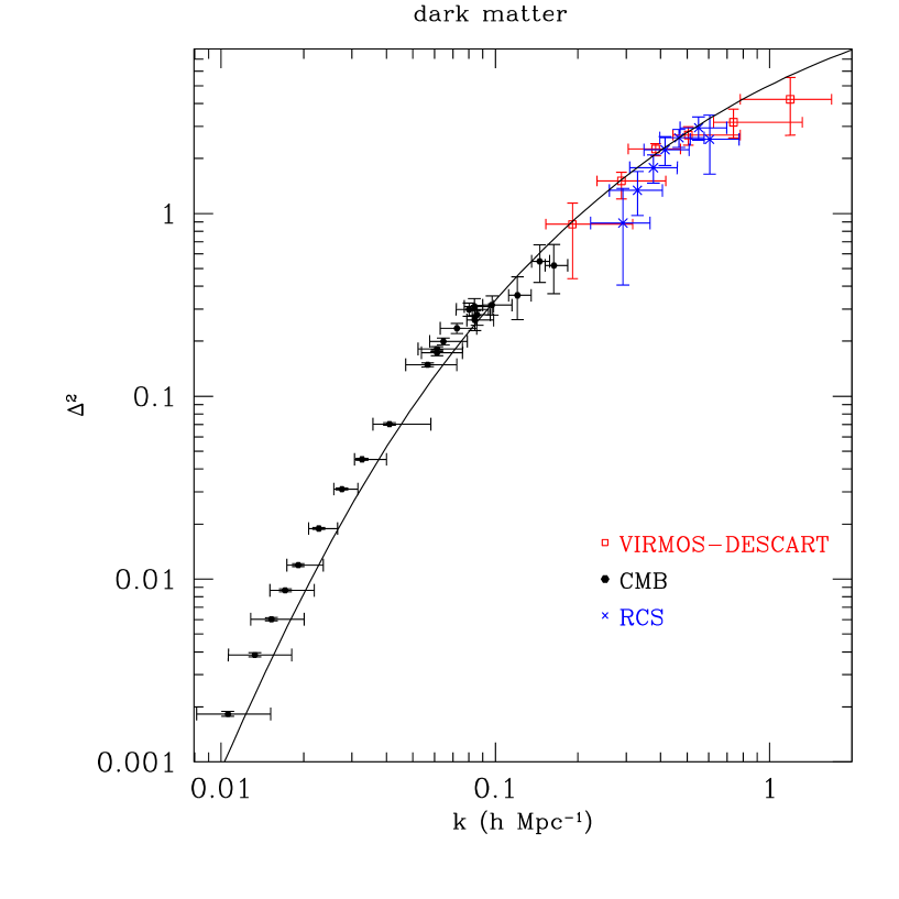
Figure 13: Linearized CMB and RCS comparison power spectrum from Tegmark & Zaldarriaga (2002). The open boxes are the VIRMOS-DESCART power. They are mutually uncorrelated. The solid boxes are a combination of CMB powers. The crosses are RCS points. The lensing data sets are linearly decompressed and evolved to $z=0$ (see text for details). The solid line is the linear LCDM model.

The resulting combined CMB and weak lensing data is shown in Figure 13. Our horizontal error bars are derived from the half width of the window function (top left panel of Figure 11). The error bars have been rescaled to the Tegmark & Zaldarriaga (2002) convention of 20% to 80% using a Gaussian model. The CMB data, courtesy of Max Tegmark, includes all the experiments compiled in Tegmark & Zaldarriaga (2002) as well as the recent WMAP data (Tegmark, private communication). We see good agreement between two completely different lensing data sets (RCS and VIRMOS-DESCART), as well as a good fit to the standard cosmological model. The residual differences could well arise from the subtleties in modelling the PD96 prescription, since we see a better fit to the same model using the Smith et al. (2002) algorithm in the non-linear power shown in the top left panel of Figure 10. Unfortunately the newer, more accurate non-linear formulae are difficult to invert from non-linear to linear power heuristically.

The CMB data can be predicted from first principles to exquisite accuracy. The weak lensing is similarly predictable from first principles, and only limited by the accuracy of simulations. These are currently not a limiting step, but do need to improve to match newer lensing data sets. Both CMB and weak lensing data sets are observationally challenging to obtain, but theoretically very clean to interpret and are unlikely to contain astronomical uncertainties. We expect ongoing surveys such as the CFHT legacy survey (http://www.cfht.hawaii.edu/Science/CFHLS/) to bring the measurement of non-linear power to a precision era, for which we can then perform precision cosmology without invoking complex poorly understood radiative phenomena.

Figure 14: The 3-D power spectrum of galaxies at redshift zero, for the minimum variance method A. The dotted line is the input power spectrum, linearly scaled from the Smith et al. (2002) power spectrum at $z_{m}=0.36$. The solid line is the deprojected 3-D power spectrum from the nonlinear projected 2-D power spectrum. The crosses are the power spectrum deprojected from the measured angular power spectrum. The shaded region is covering the deprojected 3-D power spectrum when the input redshift $z_{s}$ varies over the bootstrap uncertainty from 0.325 to 0.355. Boxes are the power spectrum from APM (Eisenstein & Zaldarriaga, 2001), small circles from 2MASS (Maller et al., 2003), and large solid circles from SDSS (Dodelson et al., 2002). The dot-dashed line is the parametrized power spectrum $(k/(0.18h{\rm Mpc}^{-1}))^{1.8}$. The dashed line is the projection/deprojection of this power law power spectrum.

5.2 galaxy and cross power spectra

The galaxy and cross power spectra are obtained completely analogously. The results for Method A are shown in Figures 14 and 15, and corresponding window functions are Figures 16 and 17. We compare our results to that obtained by inverting angular power spectra from 2MASS (Maller et al., 2003), APM (Eisenstein & Zaldarriaga, 2001) and SDSS (Dodelson et al., 2002). To compare with APM, we used table 4 of Eisenstein & Zaldarriaga (2001) and used their $(C_{P}^{-1})^{1/2}$ as error bars. In order to compare with our result, the power of APM has been linearly evolved from $z=0.11$ to zero in figure 14, which is analogous to our analysis. For SDSS, we use the data in table 2 of Dodelson et al. (2002). We used the error bar not including redshift errors, and linearly evolved every bin to redshift zero. The median weight redshifts were taken from table 1 of Dodelson et al. (2002) given by the SDSS photo-z’s. We combined the results of the 4 magnitudes bins weighted by the inverse variances.

Figure 15: The 3-D power spectrum of the cross-correlation of galaxy and dark matter at redshift zero, for method A. The box is the power spectrum deprojected from the angular power spectrum. The dotted line is the original power spectrum, linearly evolved from the Smith et al. (2002) power spectrum at $z_{m}=0.36$. The solid line is the deprojected 3-D power spectrum from the non-linearly projected 2-D power spectrum. The dot-dashed is the cross power for non-stochastic galaxies where the bias is adjusted to give a power law correlation, and the dashed line is the corresponding deprojection.

Figure 16: The window function of galaxies, for method A. ¿From bottom to top are for $k=0.24$, $k=0.48$, $k=0.96$, $k=1.92$, $k=3.84$, $k=7.68$, $k=15.36(h\rm Mpc^{-1})$, which have been moved down 0.6, 0.4, 0.2, 0, -0.2, -0.4, -0.6 units respectively.

Figure 17: Window function of the cross-correlation of galaxy and dark matter, for method A. The meaning of the lines and signs are the same as Fig. 16.

The VIRMOS-DESCART galaxies clearly show more power than the SDSS or APM data set. For reference, Figure 14 also shows the dark matter power (solid line) and the best fit $n=1.8$ power law to the angular power spectrum (dot-dashed line). In the inversion, we used the normalization coefficients ${\bf N}$ of the dark matter, which can introduce a bias for a power spectrum of different slope. The result of projecting and deprojecting the power law is shown as the long dashed curve, which is in general agreement with the input power.

To put the result in perspective, the best fit correlation length (described in section 3) is $r_{0}=4.79\pm 0.22(h^{-1}\rm Mpc)$ at median redshift $z_{m}=0.36$ for fixed power law index $n=1.8$. This is similar to correlation lengths found in CNOC2 (Shepherd et al., 2001), where the correlation length varied from $r_{0}\sim 3.4-5.5h^{-1}$ Mpc depending on galaxy population and redshift. The different power in APM and SDSS might just be a reflection of different galaxy types. The 2MASS galaxies, which are also infrared selected like the VIRMOS-DESCART, are in better agreement. We also note that overestimating galaxy distances overestimates the inferred power, and the nominal bootstrap uncertainty is reflected in the hashed region around the solid line in Figure 14. If we estimate the SDSS correlation length to be 0.3$h$Mpc^-3 linearly evolved at $z=0$, we infer a correlation length $r_{0}=3h^{-1}$ Mpc, which is at the low range for the CNOC2 sample. We should note that the overall redshift calibration could be off by more than the bootstrap error. The redshift distribution of galaxies is also broad, and we assumed a linear evolution model for the clustering, which might not be what the galaxies actually do. In principle this evolution can be measured from the data itself by modelling the galaxies at difference magnitude cutoffs, which is the subject of a future paper. In any case, this comparison puts forwards the central role of redshift information for a correct cosmological interpretation of the data

The cross power spectrum from LCDM (table 1) is shown in figure 15 as the dot-dashed line. The dashed line near it is the deprojected power spectrum from the non-linearly projection of the new cross power. The two lines are still close to each other, which means the inversion process for the cross power spectrum is also robust.

Just as for dark matter, each of the bins has correlations. Qualitatively, they are similarly behaved to that of the dark matter. We only show the cross-correlation coefficient for method A in figure 18.

Figure 18: cross-correlation coefficient using method A for the galaxy and the galaxy-dark matter cross correlation. The top panel is for galaxy, and the bottom panel is for galaxy-dark matter cross correlation. The meaning of lines are the same as Fig. 8.

With the full set of deprojected three dimensional power spectra of galaxies $\Delta^{2}_{\rm gal}$, dark matter $\Delta^{2}_{\rm dm}$, and their cross-correlation $\Delta^{2}_{\rm cross}$, we can directly measure the derived quantities “bias” $b$ and “stochasticity” $r$ (Pen, 1998). The bias is:

$$b=\sqrt{\frac{\Delta^{2}_{\rm gal}}{\Delta^{2}_{\rm dm}}}$$ (31)

which is shown in Fig.19. The upper error bars are obtained by using the $1-\sigma$ upper value for $\Delta^{2}_{\rm gal}$ divided by the $1-\sigma$ lower value of $\Delta^{2}_{\rm dm}$, and analogously for the lower error bar. From the definition, bias is dependent on the cosmology. The galaxy-dark matter cross-correlation coefficient is also directly measurable,

$$r=\frac{\Delta^{2}_{\rm cross}}{\sqrt{{\Delta^{2}_{\rm dm}}{\Delta^{2}_{\rm gal}}}}.$$ (32)

The dark matter power has the largest error bar. One can take the ratio of cross and galaxy power, which has smaller errors. We call this the “galaxy halo parameter” $h$, defined as

$$h\equiv\frac{r}{b}=\frac{\Delta^{2}_{\rm cross}}{\Delta^{2}_{\rm gal}}.$$ (33)

It is shown in the bottom panel of Fig. 19. The error bars are drawn using the procedure described above. This halo parameter is also dependent on cosmology, but the galaxy-dark matter cross-correlation coefficient is independent.

Figure 19: The top panels are bias of galaxies versus dark matter, for method A and B from left to right. The middle panels are cross-correlation coefficients of galaxy and dark matter, for method A on the left, and method B on the right. The bottom panels are the “galaxy halo parameter”. The dotted lines in the right panels are best-fit values and the shaded region show the formal uncertainty: $b=1.24\pm 0.18$, $r=0.75\pm 0.23$, $h=0.57\pm 0.16$. In our linear evolution model, the results are redshift independent.

We fitted a constant average value for $b$ from the minimum in $\chi^{2}$ for Method B:

$$\chi^{2}=\frac{1}{N}\sum_{i=1}^{N}{\frac{\left[\Delta^{2}_{\rm gal}(k_{i})-b^{2}\Delta^{2}_{\rm dm}(k_{i})\right]^{2}}{\sigma^{2}_{\rm gal}(k_{i})+b^{2}\sigma^{2}_{\rm dm}(k_{i})}}$$ (34)

sampled at six wavenumbers $k_{i}=$0.24, 0.48, 0.96, 1.92, 3.84, 7.68$h$Mpc^-1. Since the covariances are neglible, we neglected them. The variance of $b$ is taken from $\Delta\chi^{2}$,

$$\Delta\sigma_{\chi^{2}}=\frac{\sqrt{2}}{\sqrt{N}}=\frac{1}{2}\frac{d^{2}\chi^{2}}{db^{2}}(\delta b)^{2}.$$ (35)

We apply the same procedure to solve for $r$ and $h$. Formally, we find $b=1.24\pm 0.18$, $r=0.75\pm 0.23$, and $h=r/b=0.57\pm 0.16$ with $\chi^{2}=1.20,0.51,0.86$ per d.o.f. for six degrees of freedom, consistent with the expected standard deviation of 0.6. Just as the bias measurements are subject to systematic redshift calibration uncertainties, the cross-correlation results could also depend on such issues. Future surveys with photometric redshifts signficantly reduce this problem.

The resulting bias $b$ is larger than that found from comparing VIRMOS-DESCART to RCS (Hoekstra et al., 2002). That study found $b=0.71^{+0.06}_{-0.04}$ and $r=0.57^{+0.08}_{-0.07}$. The cross correlation coefficient $r$ is consistent. The apparent discrepancy in the bias $b$ should not be overinterpreted. This earlier comparison was in 2-dimensional projection. Furthermore, RCS galaxies are red R selected, which can be a different population. Within the SDSS galaxies on our scales of $k\sim 1h$Mpc^-1 the power for galaxies varies by a factor of 4 between the 18-19 and the 21-22 magnitude bin. Similarly, the 2MASS power (Maller et al., 2003) is closer to our derived value than the R selected SDSS galaxies. One clearly needs to exercise care when converting the parameter fits from one sample of galaxies to another one, as galaxies selected in different colours will have quite different clustering properties.

Our bias, cross-correlation and halo parameters were all estimated in 3-D space. One could have also attempted a parametric estimation on the 2-D projected power. For an optimal inversion process if one takes the covariances between scales into account, the results will be the same. The single biggest source of larger error is that we added the $B$ mode power to the error budget. Our model of sample variance in the optimal 2-D power will also give a larger sample variance error. The reason for that is the under-estimate of error on the 2-pt correlation function. The previous sample variance errors were estimated using an effective contiguous area. The masks and source clustering will increase the sample variance, since the same area is now non-uniformly sampled. In Figure 2, one sees that at $l$ up to 1000, sample variance makes up half the error budget (the dashed line is the noise, which exceeds the signal at $l\sim 1000$). At the end of the day we do have about twice the error bar, coming from this combination of factors.

We had checked the effects of redshift binning, and at 15 there was about a percent change compared to an infinite number of slices. The redshift evolution is parametrized, so the finer the redshift bins are the more accurate it gets. In the linear evolution model, the redshifts scale the same for the galaxies and dark matter, so that cancels exactly and is redshift invariant.

One expects galaxies and dark matter to be well correlated on linear scales when $\Delta^{2}<1$ for both galaxies and dark matter, which is not well probed by the angular scales of the current data. Newer larger surveys should significantly improve on the angular scale coverage. When the two fields are well correlated, there is no sample variance in the measurements of $r$ and $b$, which is reflected in the full joint estimation Fisher matrix. Using the current data, however, the errors in large scales are dominated by a $B$ mode, which is not easily modelled.

6 Comparison with Theory

In this section we will discuss the results of the study in the context of theories and other surveys. Measuring the relation between the distribution of light and that of dark matter has significant cosmological consequences, as discussed in the introduction. In the other direction, the theory of galaxy formation requires observational constraints to be tested. While physical cosmology originated thirty years ago in the paradigm that stars account for all the mass in the universe, today’s picture is very different. The universe appears dominated by very mysterious dark energy accounting for about 70% of the energy density of the universe. The second most important energetic contribution is dark matter, accounting for another 27%. Ordinary baryonic matter accounts for another 3%. The visible stars account for less than 0.3%. Optical power spectra of galaxies measure the distribution of this 0.3% of matter, which may or may not be a good tracer of the hundredfold more abundant dark matter. The challenge to galaxy formation models is to understand the distribution and kinematics of that small fraction of visible stars.

Different galaxies are composed of different stellar populations. Galaxies of different types cluster differently. Empirically it is known that red (early) type galaxies cluster more strongly than blue (late) type galaxies. The goal of the theory of galaxy formation is to quantify the distribution of visible galaxies, i.e. the distribution of visible light. This distribution is quantified by various statistical properties. At the two point level, theories of galaxy formation can be tested by predicting the two point statistics measured in this paper: auto and cross correlations. This correlation is a function of colour, morphology and redshift.

Semi-analytic studies generically predict (Somerville et al., 2001) earlier type (red elliptical) galaxies to be more strongly biased than late type (blue spiral) galaxies. Qualitatively, one might expect the VIRMOS-DESCART $I$ band selected galaxies to be systematically redder than SDSS or RCS galaxies, and therefore more clustered (i.e. more biased). Here we should keep in mind that the restframe colours at our median weighted redshift $z_{m}\sim 0.36$ are significantly bluer, so RCS/SDSS $R$ bands are closer to restframe $V$, while VIRMOS-DESCART $I$ shifts into the rest frame $R$. Comparison with APM or 2MASS is furthermore complicated by the significant difference in redshift distributions: these latter two surveys are much shallower with median redshifts of 0.11 and 0.07 respectively. In our comparison plot shown in Figure 14, the different redshifts were scaled using a linear evolution model. Linear evolution assumes that clustering increases due to gravitationally induced motions. In biasing models, the clustering is enhanced by creating the objects in a more clustered fashion, such that the gravitational motions have a smaller fractional effect. A biased population is expected to evolve more slowly. The 2MASS galaxies actually have significantly more power than our VIRMOS-DESCART sample. Should the picture hold that the redder surveys select for earlier type galaxies, Somerville et al. (2001) predict an increasing bias as one goes from blue to red, which is from APM to RCS/SDSS to VIRMOS-DESCART to 2MASS. The stochasticity as parametrized by the cross correlation coefficient $r$ was predicted to be less population dependent, which is what we observe.

These qualitative statements are not easy to quantify. One would need to have a common measure of galaxy morphological classification into early and late types, and correct for evolutionary effects. Empirically, a careful study of the CNOC2 survey (Shepherd et al., 2001) showed the strong dependence of the clustering amplitude on the galaxy types. The relative evolution of each population was rapid, and the early types were much more clustered than the late types.

Kochanek et al. (2000) did a morphological breakdown of the 2MASS population, and also a comparison to several other surveys. According to their estimates, the bright 2MASS sample consists of a mixture of about half early and half late type galaxies, while APM and other blue selected surveys have 20% early 80% late type galaxies. This is likely the origin for the larger power in the 2MASS survey, especially on small nonlinear scales. Brinchmann et al. (1998) measured the CFRS galaxy morphologies with HST, and also find about equal early and late type galaxies in our magnitude range. The CFRS galaxies are selected by similar colours as VIRMOS-DESCART, so we expect 2MASS and VIRMOS-DESCART to yield similar results. The difference in redshift distribution opens up some leeway, but our results are in general consistent.

The observable statistics do not end at the two point function. The full three point function and windowed skewness for the dark matter has been measured to better than 10% accuracy (Pen et al., 2003; Bernardeau et al., 2002). The cross skewness to luminous matter has 4 moments (Pen, 1998), which are all directly measurable and provide additional constraints on galaxy formation models.

We note at this point that our model for power spectrum inversion was designed with dark matter evolution in mind, which is physically well understood from first principles. We naively applied this model to the galaxy and cross-correlation power using the same assumptions, that light traces mass and that the stochasticity is small. Our results obtained under these assumptions show that the assumptions are only partially true: the optical galaxies are biased, and there is evidence for stochasticity. The galaxy halo parameter $h$ was inconsistent with unity, ruling out a mass traces light model. When light does not trace mass, as we have found, our linear evolution model used to deproject the galaxies is not a unique interpretation of the galaxy power. One could have many different plausible mechanisms which can lead to the same observed data set, but with quite different underlying properties. Even within a magnitude range, one is measuring a mixture of nearby intrinsically faint galaxies and distant intrinsically bright galaxies. It is likely that these two populations have different power, and do not evolve by any simple parametrized model. In the future, photometric redshifts will allow separation of several of these effects, and give a systematic parametrized hierarchical measure for galaxy formation.

7 The Galaxy-Dark Matter Connection

Mathematically, all two point statistics encode the same information. When we observe the distribution of dark matter and galaxies, all two point information is described by two power spectra and one cross spectrum. One can also construct derivatives of these quantities, and non-linear combinations, for example the bias and cross correlation coefficient shown in the previous sections.

Historically, the paradigm to understand dark matter was not on this equal footing, but rather centered on visible galaxies. One could measure the luminosity and number density of galaxies. A popular strategy was to attempt to measure the mass concentration associated with the light. The mass concentration is known to have a larger spatial extent than the light, which was parametrized as the radial halo mass distribution which we call the “halo profile”. If one could measure all the mass associated to halos, one could in multiply the number density of galaxies by the mass of the halos to measure the mass in the universe. Of course there could also be mass that is not associated with visible galaxies, so that would still only represent a lower limit to the mass density of the universe. We can connect these two viewpoints, which are different interpretations of the same numbers.

Several approaches exist to measure the halo mass. Perhaps the most direct is galaxy-galaxy lensing. One defines a halo profile $H(r)$, and considers each galaxy to have a halo, such that the dark matter distribution is the convolution of the position of galaxies described by a density distribution $\rho_{\rm gal}$, which may be a sum of $\delta$-functions. One further assumes that all dark matter is associated with such halos. Galaxies of different morphologies, luminosity or colour may have different halos, and one can do a full segregated measurement. The formalism remains the same, so we only consider one universal galaxy class. One then tries to fit for this universal halo profile. Apart from noise weights, all analysis proceed as follows. The distribution of “halo” dark matter is

$$\rho_{\rm halo}\equiv\int\rho_{\rm gal}(x^{\prime})H(|x-x^{\prime}|)d^{3}x^{\prime}.$$ (36)

If one sums the tangential shear to each galaxy, and stacks all such galaxies, one has cross correlated the dark matter field (36) with the galaxy field,

$$\xi_{t}(r)=\frac{\langle\rho_{\rm gal}(x)\rho_{\rm DM}(x+r)\rangle}{\bar{\rho}_{\rm gal}\bar{\rho}_{\rm DM}}.$$ (37)

In the halo model, one equates $\rho_{\rm halo}=\rho_{\rm DM}$. Formally, this yields the cross-correlation of the galaxy position with the associated halo mass. This is equivalent to Fourier transforming, and multiplying both sides of equation (36) by the galaxy density,

$$\Delta^{2}_{\rm cross}(k)=\Delta^{2}_{\rm gal}(k)h(k).$$ (38)

We have absorbed the normalization coefficients into the dimensionless halo profile $\bar{n}h(r)\equiv H(r)$ with $\bar{n}=\bar{\rho}_{\rm DM}/\bar{\rho}_{g}$. Inverse Fourier transforming and applying equation (33) we find

$$H(r)\equiv\bar{n}h(r)=4\pi\bar{n}\int\frac{r(k)}{b(k)}\frac{\sin(kr)}{kr}k^{2}dk.$$ (39)

The halo profile is mathematically equivalent to the Fourier transform of the cross correlation coefficient divided by the bias, and requires only measurements of the galaxy auto-correlation and the galaxy-dark matter cross correlation functions. It is the Fourier transform of our “galaxy halo parameter” $h$ defined in equation (33).

Formally, one could derive a mass from the halo profile $H(r)$, and compare this to masses of halos. This interpretation is parameter dependent, since the normalization in (39) depends on the mean density of galaxies, which depends on the flux limits of the survey. The deeper a survey looks, the more faint galaxies one finds, so the gravitating mass is divided by more galaxies. Similarly it is tricky to extrapolate (39) to obtain a value of the total cosmological density. One only measures the mass correlated with galaxies, and there could be more mass that does not correlate. I.e., if $r<1$, the halo may underestimates total mass.

Since all two point statistics are equivalent, measurement of “halo profiles” always measure the mass-light cross correlation. Fitting to a universal profile is mathematically equivalent to equation (39). If one knows the mean number density of galaxies, one could use this relation to infer the mean density of matter $\bar{\rho}_{\rm DM}=\bar{\rho}_{\rm gal}4\pi\int h(r)r^{2}dr=\bar{\rho}_{\rm gal}h(k=0)$ (Wilson et al., 2001). We see that the results can under or overestimate the total matter, depending on the the correlation properties of galaxies and dark matter. For the fiducial $\Omega_{0}=0.27$ model used in our analysis, the VIRMOS-DESCART halo parameter is $h=0.57\pm 0.16$, implying that about $\Omega_{\rm halo}=h\Omega_{0}\sim 0.15$ is in dark matter correlated with $I$ selected galaxies. This is consistent with the low inferred values of $\Omega_{\rm halo}$ in the literature (Wilson et al., 2001; Seljak, 2002).

A popular interpretation of the dark matter distribution has been in terms of halo models (Guzik & Seljak, 2002). When describing the distribution of galaxies, one also needs to specify the cross correlation of galaxies relative to these halos. These cross correlation coefficients must be calibrated to the observed values of the “galaxy halo parameter” $h(r)$.

8 Conclusions

We have presented the first full optimal analyses of two dimensional and deprojected 3-D power spectra of dark matter and galaxies. We used weak gravitational lensing from the VIRMOS-DESCART survey, and their relation to the galaxy distribution in the same data set. The survey is sensitive to $0.37<k<2.88h{\rm Mpc}^{-1}$ and probes the regime of non-linear clustering. We have compared the results of three different deprojection procedures, and found that our method B based on partial deconvolution is simultaneously robust, has narrow window functions, and mostly uncorrelated error bars. Full inversion is unstable, as might be expected, and a cut with SVD results in a highly tangled window function. No choice of cutoff leads to a meaningful three dimensional power spectrum for this full inversion, as measured by the covariance matrix of the solution. For the galaxy power spectrum, the inversion is more stable, but still noisy.

We tested the effects of incorrect model priors. While the true power is very non-linear, using a linear evolution model relative to the median redshift does not introduce a large error. For the dark matter power spectrum, the errors are dominated by the B-mode and shot noise. For the galaxy and cross correlation power spectrum the noise is significantly smaller, and redshift distribution errors dominate.

The deprojected dark matter distribution is consistent with that expected from the standard WMAP $\Lambda$ cosmologies with $\sigma_{8}=0.9$. The results agree well with deprojected RCS lensing data and the CMB linearly evolved power spectrum. The galaxy distribution is similar to the 2MASS galaxies, but more clustered than that found by APM and SDSS. This may be due to the different colour band selection. Using the cross correlation we confirm earlier results that galaxies and dark matter are indeed distributed stochastically on non-linear scales.

We have quantified the bias and cross-correlation coefficient $b=1.24\pm 0.18$, $r=0.75\pm 0.23$. A less noisy combination of the parameters that can be measured is the “galaxy halo parameter” $h=r/b=0.57\pm 0.16$. These parameters describe the relation between dark and luminous matter, and are the key uncertainties in the interpretation of galaxy-galaxy lensing.

All error analyses used Gaussian assumptions. Most of the regime is noise dominated, for which Gaussianity is a good approximation. For the sample variance this potentially underestimates errors (Hu & White, 2001). We plan future analyses to quantify this effect using N-body simulations. The upcoming Canada-France-Hawaii-Telescope Legacy Survey weak lensing survey should significantly improve on all measurements, and probe to larger scales. At larger scales one will be able to measure bias and stochasticity without being affected by finite field size sample variance.

References

- Bacon et al. (2002) Bacon D., Massey R., Refregier A., Ellis R., 2002, in eprint arXiv:astro-ph/0203134 Joint Cosmic Shear Measurements with the Keck and William Herschel Telescopes. pp 3134–+
- Baugh & Efstathiou (1993) Baugh C. M., Efstathiou G., 1993, MNRAS, 265, 145
- Bernardeau et al. (2002) Bernardeau F., Mellier Y., van Waerbeke L., 2002, A&A, 389, L28
- Brinchmann et al. (1998) Brinchmann J., Abraham R., Schade D., Tresse L., Ellis R. S., Lilly S., Le Fevre O., Glazebrook K., Hammer F., Colless M., Crampton D., Broadhurst T., 1998, ApJ, 499, 112
- Brown et al. (2002) Brown M. L., Taylor A. N., Bacon D. J., Gray M. E., Dye S., Meisenheimer K., Wolf C., 2002, in eprint arXiv:astro-ph/0210213 The shear power spectrum from the COMBO-17 survey. pp 10213–+
- Carroll et al. (1992) Carroll S. M., Press W. H., Turner E. L., 1992, ARA&A, 30, 499
- Contaldi et al. (2003) Contaldi C. R., Hoekstra H., Lewis A., 2003, ArXiv Astrophysics e-prints, pp 2435–+
- Crampton et al. (1995) Crampton D., Le Fevre O., Lilly S. J., Hammer F., 1995, ApJ, 455, 96
- Dodelson & Gaztañaga (2000) Dodelson S., Gaztañaga E., 2000, MNRAS, 312, 774
- Dodelson et al. (2002) Dodelson S. et al. , 2002, ApJ, 572, 140
- Eisenstein & Zaldarriaga (2001) Eisenstein D. J., Zaldarriaga M., 2001, ApJ, 546, 2
- Guzik & Seljak (2002) Guzik J., Seljak U., 2002, MNRAS, 335, 311
- Hamana et al. (2002) Hamana T., Miyazaki S., Shimasaku K., Furusawa H., Doi M., Hamabe M., Imi K., Kimura M., Komiyama Y., Nakata F., Okada N., Okamura S., Ouchi M., Sekiguchi M., Yagi M., Yasuda N., 2002, in eprint arXiv:astro-ph/0210450 Cosmic shear statistics in the Suprime-Cam 2.1 sq deg field: Constraints on Omega_m and sigma_8. pp 10450–+
- Hamilton et al. (1991) Hamilton A. J. S., Matthews A., Kumar P., Lu E., 1991, ApJ, 374, L1
- Hammer et al. (1995) Hammer F., Crampton D., Le Fevre O., Lilly S. J., 1995, ApJ, 455, 88
- Hoekstra et al. (2002) Hoekstra H., van Waerbeke L., Gladders M. D., Mellier Y., Yee H. K. C., 2002, ApJ, 577, 604
- Hoekstra et al. (2002) Hoekstra H., Yee H. K. C., Gladders M. D., Barrientos L. F., Hall P. B., Infante L., 2002, ApJ, 572, 55
- Hu & White (2001) Hu W., White M., 2001, ApJ, 554, 67
- Huterer (2002) Huterer D., 2002, Phys. Rev. D, 65, 63001
- Jarvis et al. (2002) Jarvis M., Bernstein G., Jain B., Fischer P., Smith D., Tyson J. A., Wittman D., 2002, ArXiv Astrophysics e-prints, pp 10604–+
- Kochanek et al. (2000) Kochanek K., Pahre M., Falco E., 2000, in eprint arXiv:astro-ph/0011458 Evidence for Inconsistencies in Galaxy Luminosity Functions Defined by Spectral Type. pp 11458–+
- Le Fevre et al. (1995) Le Fevre O., Crampton D., Lilly S. J., Hammer F., Tresse L., 1995, ApJ, 455, 60
- Lilly et al. (1995) Lilly S. J., Hammer F., Le Fevre O., Crampton D., 1995, ApJ, 455, 75
- Lilly et al. (1995) Lilly S. J., Le Fevre O., Crampton D., Hammer F., Tresse L., 1995, ApJ, 455, 50
- Maddox et al. (1990) Maddox S. J., Efstathiou G., Sutherland W. J., Loveday J., 1990, MNRAS, 242, 43P
- Maller et al. (2003) Maller A. H., McIntosh D. H., Katz N., Weinberg M. D., 2003, ArXiv Astrophysics e-prints, pp 4005–+
- Padmanabhan et al. (2002) Padmanabhan N., Seljak U., Pen U. L., 2002, in eprint arXiv:astro-ph/0210478 Mining Weak Lensing Surveys. pp 10478–+
- Peacock & Dodds (1996) Peacock J. A., Dodds S. J., 1996, MNRAS, 280, L19
- Pen (1998) Pen U., 1998, ApJ, 504, 601
- Pen (1999) Pen U., 1999, ApJS, 120, 49
- Pen (2003) Pen U., 2003, ArXiv Astrophysics e-prints, pp 4513–+
- Pen et al. (2002) Pen U., Van Waerbeke L., Mellier Y., 2002, ApJ, 567, 31
- Pen et al. (2003) Pen U., Zhang T., Waerbeke L. v., Mellier Y., Zhang P., Dubinski J., 2003, in eprint arXiv:astro-ph/0302031 Detection of dark matter Skewness in the VIRMOS-DESCART survey: Implications for Omega_0. pp 2031–+
- Press et al. (1992) Press W. H., Teukolsky S. A., Vetterling W. T., Flannery B. P., 1992, Numerical recipes in FORTRAN. The art of scientific computing. Cambridge: University Press, —c1992, 2nd ed.
- Refregier et al. (2002) Refregier A., Rhodes J., Groth E. J., 2002, ApJ, 572, L131
- Seljak (1998a) Seljak U., 1998a, ApJ, 503, 492
- Seljak (1998b) Seljak U., 1998b, ApJ, 506, 64
- Seljak (2002) Seljak U., 2002, MNRAS, 337, 774
- Shepherd et al. (2001) Shepherd C. W., Carlberg R. G., Yee H. K. C., Morris S. L., Lin H., Sawicki M., Hall P. B., Patton D. R., 2001, ApJ, 560, 72
- Smith et al. (2002) Smith R. E., Peacock J. A., Jenkins A., White S. D. M., Frenk C. S., Pearce F. R., Thomas P. A., Efstathiou G., Couchmann H. M. P., Consortium T. V., 2002, ArXiv Astrophysics e-prints, pp 7664–+
- Somerville et al. (2001) Somerville R. S., Lemson G., Sigad Y., Dekel A., Kauffmann G., White S. D. M., 2001, MNRAS, 320, 289
- Spergel et al. (2003) Spergel D. N., Verde L., Peiris H. V., Komatsu E., Nolta M. R., Bennett C. L., Halpern M., Hinshaw G., Jarosik N., Kogut A., Limon M., Meyer S. S., Page L., Tucker G. S., Weiland J. L., Wollack E., Wright E. L., 2003, ArXiv Astrophysics e-prints, pp 2209–+
- Tegmark (1997a) Tegmark M., 1997a, ApJ, 480, L87+
- Tegmark (1997b) Tegmark M., 1997b, Phys. Rev. D, 55, 5895
- Tegmark & de Oliveira-Costa (2001) Tegmark M., de Oliveira-Costa A., 2001, Phys. Rev. D, 64, 63001