Fast Power Spectrum Estimation

Abstract

We present a new algorithm to rapidly and optimally compute power spectra. This new algorithm is based on a generalization of iterative multigrid, and has computational cost ${\cal O}(N\log N)$, compared to the standard brute force approach which costs ${\cal O}(N^{3})$. The procedure retains this speed on the full sky and for ill-conditioned matrices. It is applicable to galaxy power spectra, CMB, polarization and weak lensing data. We present a mathematical convergence analysis, and performance results.

1 Introduction

Cosmological data sets are rapidly becoming very large, making the optimal analysis of data a challenging problem. Particularly large problems arise in the analysis of CMB data, galaxy power spectra and weak lensing data. For Gaussian random fields, the statistics are fully solvable, and the construction of optimal quadratic or maximum likelihood estimators is uniquely defined.

A full maximum likelihood analysis of COBE which contained 3890 pixels was done by Bunn & White (1997). The optimal analysis procedure requires ${\cal O}(N^{3})$ operations for $N$ data points, which is generally very expensive, and prohibitive for many data sets. Data compression is possible through the use of a Karhunen-Loeve expansion in terms of “signal-to-noise” eigenmodes (Bond, 1995). The first compression step still costs $O(N^{3})$, but subsequent analyses are accelerated. Faster procedures have been suggested, usually at the expense of optimality. The computation of correlation functions, for example, only costs ${\cal O}(N\log N)$ operations, and has been a popular quick algorithm (Pen et al., 2002; Szapudi et al., 2001). Similarly, a weighted Fourier Transform of the data is equally fast, and was proposed by Feldman et al. (1994). Pen et al. (2003) summarized the trade-off made in these approximations.

We consider a power spectrum estimator optimal if it minimizes the variance. The variance of the power is a four point function, which can be expressed in terms of two point functions for a Gaussian random field. One can show that a naive quadratic estimator applied to the Wiener filtered data set is optimal (Seljak, 1998). If the noise and signal covariance matrices commute, the correlation function and weighted Fourier techniques are optimal. If the signal-to-noise is less than unity on all scales, the correlation function is optimal. But in general none of these cases applies, in which case the historic fast estimators are suboptimal.

In this paper we present an algorithm which is fast and optimal, and works on a wide range of problems, geometries, and condition numbers. It is an extension of the iterative technique presented in Padmanabhan et al. (2002) to cover regimes of poor condition number.

The basic premise is that the forward operation of applying the signal and noise correlations to the data set an be done in ${\cal O}(N\log N)$ time. We then construct iterative techniques to achieve the inverse.

2 Maximum Likelihood

In this section we review the mathematical formulation of the power spectrum estimation problem. An observation is a data set of $N$ points sampled at positions $x_{i}$, written as a vector $\Delta_{i}$. We take this vector to have zero expectation value. This vector is assumed to be the sum of signal plus noise, such that the expectation of the covariance matrix is

$$\langle\Delta_{i}\Delta_{j}\rangle=C^{N}_{ij}+C^{S}_{ij}$$ (1)

for a noise covariance matrix ${\bf C}^{N}$ and a signal covariance ${\bf C}^{S}$. We parametrize the signal covariance matrix as a sum of $n_{b}$ band powers,

$${\bf C}^{S}=\sum_{\alpha=1}^{n_{b}}p_{\alpha}{\bf C}_{\alpha}.$$ (2)

The log of the probability of the data given a model is

$${\cal L}=-\frac{1}{2}\log|{\bf C}^{N}+{\bf C}^{S}|-\frac{\Delta^{T}({\bf C}^{N}+{\bf C}^{S})^{-1}\Delta}{2}+\frac{n_{b}}{2}\log(2\pi)$$ (3)

We wish to find the set of parameters $p_{\alpha}$ which maximize the likelihood (3). Differentiating, one obtains a system of equations

$$-{\rm Tr}[({\bf C}^{N}+{\bf C}^{S})^{-1}{\bf C}_{\alpha}]+\Delta^{t}({\bf C}^{N}+{\bf C}^{S})^{-1}{\bf C}_{\alpha}({\bf C}^{N}+{\bf C}^{S})^{-1}\Delta=0.$$ (4)

The Newton-Raphson solution for (4) starts with an initial guess $p_{\alpha}^{0}$ and iterates

$$p_{\beta}^{n+1}=p_{\beta}^{n}-f_{\alpha}G^{-1}_{\alpha\beta}$$ (5)

where $f_{\alpha}$ is the left hand side of (4) and ${\bf G}$ is the Jacobian

$$G_{\alpha\beta}=2F_{\alpha\beta}-\Delta^{t}({\bf C}^{N}+{\bf C}^{S})^{-1}{\bf C}_{\alpha}({\bf C}^{N}+{\bf C}^{S})^{-1}{\bf C}_{\beta}({\bf C}^{N}+{\bf C}^{S})^{-1}\Delta-\Delta^{t}({\bf C}^{N}+{\bf C}^{S})^{-1}{\bf C}_{\beta}({\bf C}^{N}+{\bf C}^{S})^{-1}{\bf C}_{\alpha}({\bf C}^{N}+{\bf C}^{S})^{-1}\Delta.$$ (6)

${\bf F}$ is the Fisher matrix defined as

$$F_{\alpha\beta}\equiv\frac{1}{2}{\rm Tr}[({\bf C}^{N}+{\bf C}^{S})^{-1}{\bf C}_{\beta}({\bf C}^{N}+{\bf C}^{S})^{-1}{\bf C}_{\alpha}].$$ (7)

Newton-Raphson only convergences in the domain where the sign of the curvature does not change. But even for one degree of freedom, the Gaussian likelihood encounters an inflection point. Consider

$$2\log{\cal L}=-\log(2\pi)-2\log(\sigma)-\frac{\Delta^{2}}{\sigma^{2}}.$$ (8)

We solve the equation

$$f(\sigma)\equiv\frac{1}{\sigma}-\frac{\Delta^{2}}{\sigma^{3}}=0.$$ (9)

The solution is $\sigma^{2}=\Delta^{2}$, as one would expect. In one dimension the Jacobian is the derivative, $f^{\prime}(\sigma)=-1/\sigma^{2}+3\Delta^{2}/\sigma^{4}$, which changes sign when $\sigma^{2}=3\Delta^{2}$. So the Newton-Raphson iteration (5) moves towards the correct root for guesses within a factor of 3 the true solution, but moves towards infinity for guesses that are too large.

An alternate representation is in terms of weighted quadratic estimators, where one first weights data by ${\bf W}$ and defines raw estimators $q_{\alpha}$ as

$$q_{\alpha}\equiv\Delta^{t}{\bf W}^{t}{\bf C}_{\alpha}{\bf W}\Delta-{\rm Tr}[{\bf W}{\bf C}_{\alpha}{\bf W}C_{N}].$$ (10)

The estimators of power $\tilde{p}_{\alpha}=F^{-1}_{\alpha\beta}q_{\beta}$. A Wiener filter choice is ${\bf W}=({\bf C}^{N}+{\bf C}^{S})^{-1}$. If interpreted in terms of the maximum likelihood iteration (5), it amounts to an initial guess $p_{\beta}^{0}=0$, with residual $f_{\alpha}=q_{\alpha}$. We used the expectation value $\langle{\bf G}\rangle={\bf F}$. This converges after a single iteration. Of course, we had assumed that we already knew the optimal weights for the Wiener filter. The quadratic estimator (10) does not have convergence limitations. One can start with an approximate guess for the covariance ${\bf C}^{S}$, and iterate.

In both the maximum likelihood and the quadratic estimation processes, a number of expensive operations are required. The most common one is the solution to the Wiener filter, $({\bf C}^{N}+{\bf C}^{S})^{-1}\Delta$. We will discuss in section 3 how to achieve using a fast algorithm, after which we only need to address the trace evaluation, which we do in section 6.

3 Iterative Solution

For stationary processes, the correlation matrices depend only on the separation distance between points. This makes them diagonal in Fourier space. Noise matrices are often diagonal in real space, or in a time stream space. For now we assume that a fast ${\cal O}(NlogN)$ method exists to evaluate the forward operation. In section 7 we present several fast procedures which imlement this.

For concreteness, we assume that the signal correlation is a diagonal matrix in Fourier space, while the noise matrix is diagonal in real space. We concentrate on the problem

$$({\bf S+N})x=y.$$ (11)

The first requirement is that (11) can be evaluated quickly. This is demonstrated for a range of problems in section 4. We will express all vectors in real space. We can evaluate $y$ in ${\cal O}(N\log(N))$ operations as $y={\bf N}x+{\bf S}x$. The underrelaxed Jacobi iterative solution is

$$x^{n+1}=x^{n}+(\bar{S}{\bf I}+{\bf N})^{-1}\left[y-({\bf S}+{\bf N})x^{n}\right].$$ (12)

$\bar{S}$ is our relaxation parameter, to be determined below. Define the error of the $n-$th iteration as the difference between the true solution $x$ and the current guess, $e^{n}=x^{n}-x$. Substituting into (12), we have

$$e^{n}=\left[{\bf I}-(\bar{S}{\bf I}+{\bf N})^{-1}({\bf S+N})\right]^{n}e^{0}\equiv{\bf E}^{n}e^{0}.$$ (13)

${\bf E}$ is called the error matrix. We define the spectral radius of a matrix ${\bf M}$ as $\rho({\bf M})$ to be the maximum absolute eigenvalue of ${\bf M}$. Since $\rho({\bf A+B})\leq\rho({\bf A})+\rho(\bf{B})$, the sufficient condition for (13) to converge is

$$\bar{S}\geq\rho({\bf S}).$$ (14)

We can prove (14) by expanding the matrix product in (13) into two positive definite terms each with spectral radius less than unity, $\rho[(\bar{S}{\bf I}+{\bf N})^{-1}{\bf N}]<1$ and $\rho[(\bar{S}{\bf I}+{\bf N})^{-1}{\bf S}]<1$. The first inequality is trivial since the two terms are simultaneously diagonal. The second inequality follows by expanding its inverse, and noting that the smallest eigenvalue of the inverse is larger than one.

When ${\bf N}$ is diagonal, we obtain optimal convergence with $\bar{S}=(S_{0}+S_{\infty})/2$, i.e. the average of the largest and smallest eigenvalue of the noise matrix. For practical purposes, we have never encountered convergence problems with this choice, and always found better convergence than using the hard bound (14).

In real space, (13) can be visualized as follows. We take an error vector $e^{n}$, multiply one copy by the pixel noise, and convolve another copy with the two point correlation function. We add the two resulting vectors, and divide by the pixel noise plus a constant corresponding to the amplification factor for the wave with the largest signal power. We then subtract this from the original vector $e^{n}$. The convergence is rapid if it pointwise converges to zero. The pixels which are slowest to converge are those where the noise is much smaller than $\bar{S}$ when we inject a wave corresponding to the smallest eigenvalue of the signal correlation. The worst pixel converges as

$$|e^{n}|_{\infty}\propto[1-(N_{0}+S_{0})/(N_{0}+\bar{S})]^{n}$$ (15)

where $N_{0}$ is the smallest eigenvalue of ${\bf N}$, $S_{0}$ is the smallest eigenvalue of ${\bf S}$, and $\bar{S}$ is the largest eigenvalue. It takes $\sim(N_{0}+\bar{S})/(N_{0}+S_{0})$ steps to decrease the error by an $e$-fold. The rate is related to the condition number of ${\bf S}$, and the lower limit for ${\bf N}$. It is apparent that choosing $\bar{S}$ larger than necessary slows the convergence down.

The convergence rate is limited by the condition number of ${\bf S}+{\bf N}$. Consider the problem of power spectrum estimation on an irregular region with constant noise. We can express this problem on a larger enclosing domain, and write $N^{-1}_{ii}=0$ on the padding region. ${\bf N}^{-1}$ is not invertible in this case. But we can write

$$({\bf S}{\bf N}^{-1}+{\bf I}){\bf N}x=y.$$ (16)

Setting $u={\bf N}x$, we first solve (16) for $u$, and then evaluate $x={\bf N}^{-1}u$, where zero entries on the diagonal of ${\bf N}^{-1}$ becomes a non-problem. The problem instead arises when the noise is small. Large and small is defined relative to the signal. Since the signal covers a spectrum of values, we shall use the mean value $S_{M}$ as reference point. We factor ${\bf N}={\bf H}{\bf L}$, where ${\bf H}={\bf N}$ when ${\bf N}>S_{M}$ and equal to one otherwise. We can now generalize (16) to

$$({\bf S}{\bf H}^{-1}+{\bf L}){\bf H}x=y,$$ (17)

and define $u={\bf H}x$. The iterative solution becomes

$$u^{n+1}=u^{n}+(\bar{S}{\bf H}^{-1}+{\bf L})^{-1}\left[y-({\bf S}{\bf H}^{-1}+{\bf L})u^{n}\right].$$ (18)

The convergence criterion (14) is still a sufficient condition for the Jacobi iteration (18), but may be quite non-optimal. We can instead use an iterative estimate of $\bar{S}=\rho({\bf S}{\bf H}^{-1})$ using a power iteration. To prove the convergence of (18), we use the same argument as for (14), with the second inequality holding since ${\bf H}{\bf S}^{-1}{\bf H}^{-1}$ is a similarity transformation on ${\bf S}$ which preserves eigenvalues. Should ${\bf S}$ have a large dynamic range, we can similarly factor it ${\bf S}={\bf T}{\bf U}$

$$({\bf T}{\bf H}^{-1}+{\bf U}^{-1}{\bf L}){\bf H}x={\bf U}^{-1}y,$$ (19)

with an iteration

$$u^{n+1}=u^{n}+(\bar{T}{\bf H}^{-1}+\bar{U}^{-1}{\bf L})^{-1}\left[y-({\bf T}{\bf H}^{-1}+{\bf U}^{-1}{\bf L})u^{n}\right].$$ (20)

A similar argument shows this to be a convergent iteration if we choose $\bar{T}=\rho(T)$ and $\bar{U}=1/\rho({\bf U}^{-1})$.

The iterative approach also allows us to compute the $\chi^{2}=\Delta^{T}({\bf C}^{N}+{\bf C}^{S})^{-1}\Delta$ of the solution iteratively, as well as any expression involving the contraction of vectors, such as (10). The likelihood itself requires computing a determinant, which does not fall into this framework. The trace evaluations needed in Equations (4,6) will be addressed below.

4 Convolution and boundaries

4.1 Multi-level FFT

Consider a point set contained within an irregular domain $\Omega$ with isolated boundary conditions. We imbed this domain $\Omega$ in the smallest enclosing rectangle $L$. The multiplication by the signal matrix is just a convolution by the correlation function with isolated boundary conditions, which can be performed using an FFT on a domain twice as wide as $L$. The operation $y={\bf S}x$ sets the value at every point $y_{i}$ to the sum over all points $x$ weighted by the correlation function at the separation. We can map any discrete set of points onto a regular grid using an interpolation of some order (Hockney & Eastwood, 1988).

For this iterative technique, we only rely on each of the forward operations to be evaluated rapidly. The operation of the signal on the data can always be performed in ${\cal O}(N\log N)$ time on a spatial grid by considering it a convolution, which can be performed on a tree, even if the geometry is complex, the coordinate system is unevenly sampled, or the coordinates are otherwise not appropriate for a Fourier transform, for example on the celestial sphere. Again, several methods are possible, with tradeoffs in complexity of the algorithm against computational time. As discussed in Padmanabhan et al. (2002), several levels of grids can be employed to accelerate the process. Open boundaries can be implemented, and one can add short range pair summations, much in analogy to N-body codes (Hockney & Eastwood, 1988). If correlations on a whole sphere are desired, a spherical harmonic transform can be applied for convolutions on the coarse grid followed by FFT’s on the fine grids. While spherical harmonic transforms cost ${\cal O}(N^{3/2})$, the base is only the number of coarse grid cells, and one expects to be dominated by the ${\cal O}(N\log N)$ of the fine grid in general.

4.2 Tree

Just as in N-body simulations, the optimal algorithm depends on the clustering of points. An alternative way of evaluating the signal correlation applied to a data vector ${\bf S}\Delta$ is through tree summation. This approach is very general, and does not slow down under strong clustering. A stationary signal correlation is a convolution, and we can express it as

$$u(\vec{x}_{i})\equiv{\bf S}\Delta=\sum_{j}\Delta(\vec{x}_{j})G(|\vec{x}_{i}-\vec{x}_{j}|).$$ (21)

While Equation (21) is an $N^{2}$ process, we note that it can be approximated to high accuracy through a multipole expansion. Points can be bunched together into nodes. Each node has the mean position of its constituent points (center of mass), a quadrupole moment, and the sum the masses. So instead of summing over all points, it is sufficient to sum over a smaller number of nodes. Let us describe the mass distribution of node $k$ by $\rho_{k}(\vec{x})$. The convolution over the node is

$$u(\vec{x}_{i}) \equiv {\bf S}\Delta=\sum_{k}\int dx\rho_{k}(\vec{x})G(|\vec{x}_{i}-\vec{x}|)$$ (22)

$$= \sum_{k}\left[M_{k}G(|\vec{x}_{i}-\vec{x}_{k}|)+\int\rho_{k}(\vec{x})r^{\alpha}r^{\beta}\partial_{\alpha}\partial_{\beta}G(|\vec{x}_{i}-\vec{x}_{k}|)+{\cal O}(G^{\prime\prime\prime})\right].$$

The mass $M_{k}=\int\rho_{k}$, and dipole term was cancelled by the choice $\langle\vec{x}_{k}\rangle=\frac{1}{M_{k}}\int\vec{x}\rho_{k}(\vec{x})$, and The second term in (22) can be rewritten in terms of the quadrupole moments $Q_{\alpha\beta}=\int r^{\alpha}r^{\beta}\rho_{k}$ with $r^{\alpha}=\vec{x}^{\alpha}_{k}-\vec{x}^{\alpha}$ as

$$u(\vec{x}_{i})=\sum_{k}\left\{M_{k}G(|\vec{x}_{i}-\vec{x}_{k}|)+Q_{\alpha\beta}^{k}\left[(\delta_{\alpha\beta}-\hat{r}^{\alpha}\hat{r}^{\beta})\frac{G^{\prime}(|\vec{x}_{i}-\vec{x}_{k}|)}{|\vec{x}_{i}-\vec{x}_{k}|}+\hat{r}^{\alpha}\hat{r}^{\beta}G^{\prime\prime}(|\vec{x}_{i}-\vec{x}_{k}|)\right]+{\cal O}(G^{\prime\prime\prime})\right\}.$$ (23)

$\hat{r}\equiv\vec{r}/|r|$ is the unit separation between the target point and the node center of mass. By comparing the quadrupole to the monopole, we obtain an estimate of the error in the truncation. Should this error be larger than our tolerance, we break the sum into subcomponents of the node.

The tree needs only be constructed once, so we should invest sufficient computing resources into this step to minimize the truncation errors arising from the tree. One starts by defining a top node, which includes all points. Since our goal is to maximize locality of particles, we shall subdivide each node by cutting it in half by a line perpendicular to the major axis of the quadrupole. We want to place the cut such that the quadrupole of the subnodes is minimized. This cut line can be determined through bisection. One first cuts through the center of mass, and determines the quadrupole of each subnode. We then displace the cutline towards the node with the larger quadrupole. Let $r_{m}=\sqrt{\lambda_{\rm max}}$ be the square root of the largest eigenvalue of the parent node. We then displace the cutting line by an amount proportional to $r_{m}$ times 1 minus the ratio of quadrupoles of the subnodes. We repeat this process on each subnode until each node contains exactly one point. The resulting binary tree is not balanced, since the number of particles in each child node is not equal. The depth of the tree is not determined in advance.

The truncation error in the quadrupole tree for a power law correlation function $G(R)\propto R^{-n}$ is

$$e\propto\frac{r_{m}^{3}G^{\prime\prime\prime}(R)}{G(R)}=n(n+1)(n+2)\left(\frac{r_{m}}{R}\right)^{3}.$$ (24)

Reducing $r_{m}$ by a factor of two reduces the error by a factor of 8. But the quadrupole is proportional to the node area, so the computational cost has increased a factor of 4. Let $n_{2}$ be the number of desired binary digits of accuracy. Then the quadrupole truncated tree has a computational cost $\propto(2^{n_{2}})^{2/3}$. If very high accuracy is desired, one should go to high multipole order. An order $n_{O}$ multipole evaluation in two spatial dimensions costs ${\cal O}(n_{O})$ operations, so the total node cost $\propto n_{O}^{2}$. At high multipole moments, it makes sense to reduce the node size $r_{m}$ since we gain rapidly. The optimal $n_{O}$ is thus slightly smaller than $n_{2}$. Asymptotically, the cost of the tree slightly less than $n_{2}^{2}$.

A simple tree decomposition to implement does not use the quadrupole information. For each node, we find the particle which is furthest from the center of mass. We store this distance with each node. We subdivide the node into two subnodes by a cut perpendicular to the line connecting the furthest particle to the center of mass. The cut is chosen such that the two subnodes have an equal number of particles. When walking the tree, we check that the maximal radius of the node is sufficiently smaller than the distance to the node. This tree is faster to build, since no quadrupole evaluations are required, and for each node the bisection only costs linear time in the number of particles in the node. It also minimizes the worst case error at each node.

5 Multiscale Acceleration

The convergence rate of equation (18) is primarily limited by the condition number of ${\bf S}$, since the relaxation parameter $\bar{S}$ is yields rapid convergence on modes with correlation power close to $\bar{S}$. We can, for example, project the error ${\bf e}$ onto the eigenvectors of ${\bf S}$. Since we chose $\bar{S}$ to be the largest eigenvalue of ${\bf S}$, the corresponding eigenvector converges to zero error after one iteration. We thus consider breaking the iterative solution into blocks of the eigenspace of ${\bf S}$, for which the corresponding eigenvalues have a small dynamic range. If we can use a different relaxation parameter for each block, the iteration proceeds rapidly. Let us write a complete set of $n_{b}$ band power projection operators ${\bf P}_{i}$ which sum to the identity matrix. Multiplication by the projection can also be expressed as a convolution, for which the tree algorithm described above can also be used. We generalize the iteration from equation (20)

$$u^{n+1}=u^{n}+\sum_{i}(\bar{T}_{i}{\bf H}^{-1}+\bar{U}_{i}^{-1}{\bf L})^{-1}{\bf P}_{i}\left[y-({\bf T}{\bf H}^{-1}+{\bf U}^{-1}{\bf L})u^{n}\right].$$ (25)

The error on the iteration is again

$$e^{n}=\left[{\bf I}-\sum_{i}(\bar{T}_{i}{\bf H}^{-1}+\bar{U}_{i}^{-1}{\bf L})^{-1}{\bf P}_{i}({\bf T}{\bf H}^{-1}+{\bf U}^{-1}{\bf L})\right]^{n}e^{0}.$$ (26)

We set the relaxation parameters $\bar{T}_{i}=\rho(P_{i}{\bf T})+T_{\infty}$ and $\bar{U}_{i}=1/\rho(P_{i}{\bf U}^{-1})+U_{\infty}$. In the continuous Fourier decomposition limit, we have

$$e^{n+1}(x)=e^{n}(x)-\int d^{2}kd^{2}x^{\prime}\exp[i{\bf k}\cdot({\bf x}-{\bf x}^{\prime})]\frac{P({\bf k})+N({\bf x}^{\prime})}{P({\bf k})+N({\bf x})}e^{n}({\bf x}^{\prime}).$$ (27)

The error matrix (27) is zero on the diagonal. If there is no signal, $P(k)=0$, the error matrix is zero everywhere, and the convergence is exact after one iteration. When the signal is dominant, we can neglect $N(x)$, and the error matrix is again zero. Similarly, the error matrix is zero for two elements whenever $N(x^{\prime})=N(x)$.

We can solve the error matrix exactly for two degrees of freedom. In this case, we write the noise matrix as

$${\bf N}=\left(\begin{array}[]{cc}n_{1}&0\\ 0&n_{2}\end{array}\right).$$ (28)

The orthogonal Fourier transform matrix ${\bf F}$ is

$${\bf F}=\frac{1}{\sqrt{2}}\left(\begin{array}[]{cc}1&1\\ 1&-1\end{array}\right).$$ (29)

We have two projection matrices

$${\bf P}_{1}=\left(\begin{array}[]{cc}1&0\\ 0&0\end{array}\right),\ \ \ \ \ {\bf P}_{2}=\left(\begin{array}[]{cc}0&0\\ 0&1\end{array}\right).$$ (30)

The signal correlation matrix is

$${\bf S}={\bf F}^{-1}\left(\begin{array}[]{cc}s_{1}&0\\ 0&s_{2}\end{array}\right){\bf F}.$$ (31)

The error expression is then

$$e^{n}=\left\{{\bf I}-[((s_{1}+s_{\infty}){\bf I}+{\bf N})^{-1}{\bf F}^{-1}{\bf P}_{1}+((s_{2}+s_{\infty}){\bf I}+{\bf N})^{-1}{\bf F}^{-1}{\bf P}_{2}]({\bf S}{\bf F}+{\bf F}{\bf N})\right\}^{n}e^{0}$$ (32)

For $s_{\infty}=0$, the eigenvalues of this expression can be directly evaluated

$$\lambda=\pm i\frac{(n_{1}-n_{2})(s_{1}-s_{2})}{\sqrt{(n_{1}+s_{1})(n_{2}+s_{2})(n_{1}+s_{2})(n_{2}+s_{1})}}.$$ (33)

If we take $n_{i}$ and $s_{i}$ to be sorted positively in ascending order, we see the qualitative features of the convergence. Convergence is very rapid if either ${\bf N}$ or ${\bf S}$ is well conditioned. It is poor if $n_{1}+s_{1}$ is very small compared to all the other differences in the problem, and can even fail to converge if $|\lambda|>1$. To treat the most extreme case, we set $s_{1}=n_{1}=0$. Then the iteration (32) will converge optimally for $s_{\infty}\sim{\rm min}(s_{2},n_{2})$, and the maximal eigenvalue is $\lambda<1/2$ for any choice of $n_{2},s_{2}$. At least in this scenario, we have shown that even this potentially extremely ill-conditioned system converges rapidly, better than a factor of two on each iteration.

In the continuum limit (27), we can estimate convergence in some limiting cases. If $N(x^{\prime})\gg P(k)$ is large the $k$ integral turns the power spectrum into a correlation function, $\xi({\bf x}^{\prime}-{\bf x})/N({\bf x}^{\prime})$, while if it is very small, the matrix element is given by the inverse correlation function $N({\bf x})\xi^{-1}({\bf x}-{\bf x}^{\prime})$. In either case, the matrix is very small.

When the signal matrix contains a large number of zero entries, setting $T_{\infty}$ to the mean value of the noise appears to be a robust choice. In general, we break the sum (26) into $\log_{2}(||{\bf S}||)$ terms, each of which costs ${\cal O}(N\log N)$ operations.

To test these concepts, we implemented a one dimensional example. 65536 grid points were used with periodic boundary conditions, and a power law signal correlation function $P(k)=256/k$, where $k$ is the integer wave number on the grid. The noise variance in each grid point is a random number chosen uniformly from 0.35 to 1.35. We first run the straight iteration (12) for 500 iterations. The vector $\vec{x}$ was chosen randomly, from which $\vec{y}$ was computed. We define the scaled infinity error $e_{\infty}=|x^{n}-x|_{\infty}\sqrt{65536/\sum x_{i}^{2}}$. This error is plotted as boxes in figure 1.

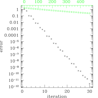
Figure 1: Convergence of Jacobi iteration and multiscale acceleration. Bottom horizontal label is the number of the iteration for the multiscale accelerated method, while the top axis is the iteration number for direct Jacobi iteration. The problem had $65536$ variables.

In this situation, we have $\bar{S}\sim 128$, $S_{0}=1/256$ and $N_{0}=0.35$. From equation (15) we expect to take up to about 366 iterations to reduce the error by an $e$-fold. This is consistent with the performance seen in figure 1.

Then we applied the multiscale accelerated iteration (25). We chose 16 bands, so the computational cost is about 16 times higher, but the convergence is much better as we see in the crosses in figure 1. The two sets of points have comparable computational cost, and the multiscale converges much better. We note that the convergence rate for the Jacobi iteration scales as the condition number, which is proportionate to the number of grid points, while the multiscale convergence is independent of that. The Jacobi iteration is still very fast compared to a brute force $N^{3}$ solution of this problem. Each of the iterative methods here take a matter of minutes on a workstation, while a brute force method takes of order a year.

It is instructive to compare this multiscale approach to traditional multigrid aceleration methods. We solve an arbitrary linear equation

$${\bf L}u=b$$ (34)

for some linear operator ${\bf L}$. The simplest procedure applies a Jacobi iteration

$$u^{n+1/2}=\left(1-{\bf D}^{-1}{\bf L}\right)u^{n}+{\bf D}^{-1}b,$$ (35)

where ${\bf D}$ is the diagonal part of ${\bf L}$. We then have a restriction operator ${\cal R}$ which maps the vector $u$ onto a coarser vector $u_{1}={\cal R}u$. In this coarser space, we need to have a coarsened version of the operator, denoted $\tilde{{\bf L}}$, for which we now solve the coarsened system

$$\tilde{{\bf L}}u_{1}^{n+1/2}=\Delta b_{1}^{n+1}\equiv{\cal R}(b-{\bf L}u^{n+1/2}).$$ (36)

One recursively applies multigrid to this coarsened system. For purposes of analysis, we assume that the coarse grid equation (36) was solved exactly. We inject this coarse grid correction using the coarse-to-fine grid prolongation operator ${\cal P}$

$$u^{n+1} = {\cal P}\tilde{{\bf L}}^{-1}\Delta b^{n+1/2}+u^{n+1/2}$$ (37)

$$= u^{n}+\left[{\cal P}\tilde{{\bf L}}^{-1}{\cal R}(1-{\bf D}^{-1}{\bf L})+{\bf D}^{-1}\right](b-{\bf L}u^{n}).$$

The error can be written as

$$e^{n}=\left[(1-{\cal P}\tilde{{\bf L}}^{-1}{\cal R}{\bf L})(1-{\bf D}^{-1}{\bf L})\right]^{n}e^{0}.$$ (38)

The standard Jacobi iteration only has the right term in parenthesis. For the Laplace operator ${\bf L}=\nabla^{2}=-k^{2}$, we can see in Fourier space that this term is dominated by small $k$, i.e. large scales, for which the term is unity, and convergence is slow. But on large scales, the restriction and prolongation operators basically commute with everything, and the first term is very small. So we see that convergence is rapid on all scales for the Laplace operator.

In correlation problems, the linear operator is typically an inverse power of the wave number, $L\sim k^{-n}$, for which the large scales actually converse rapidly, but the small scales don’t. On these small scales, the prolongation and restriction operators introduce large errors, and the convergence is not aided by this multigrid decomposition. One can remedy this problem by multiplying both sides of the equation by a sufficiently large power of $k$. Or one can recast the equation (11) as $({{\bf S}^{-1}+{\bf N}^{-1}}){\bf N}x={\bf S}^{-1}y$, and solve the system using only inverse matrices. But as we had seen in equations (15,33), the convergence is generally limited by a bad condition number on the noise matrix ${\bf N}$. Let us consider the above 2x2 example, choosing the case when $n_{1}=s_{1}=0$. For the coarse grid, the only conceivable operator is the scalar $\tilde{{\bf L}}=(s_{2}+n_{2})/2$. The restriction to a one cell coarse grid is the average of the two cells, and vice versa. The iterator error (38) is then

$$e^{n}={\bf E}^{n}e^{0}\equiv\left[\left(\begin{array}[]{cc}1&-\frac{n_{2}}{s_{2}+n_{2}}\\ 0&\frac{s_{2}}{s_{2}+n_{2}}\end{array}\right)\left(\begin{array}[]{cc}0&-1\\ -\frac{s_{2}}{s_{2}+2n_{2}}&0\end{array}\right)\right]^{n}e^{0}.$$ (39)

The term in the right parentheses is the error for a standard Jacobi iteration without multigrid, and the left term is the multigrid acceleration. In a pure Jacobi iteration, the eigenvalues are $\lambda=\pm\sqrt{\frac{s_{2}}{s_{2}+2n_{2}}}$, which tends to 1 as $n_{2}$ tends to zero and is thus slowly convergent in some cases. The combined error matrix has eigenvalues $\lambda=\frac{s_{2}(n_{2}\pm i\sqrt{3n_{2}+2s_{2}}\sqrt{5n_{2}+2s_{2}})}{2(n_{2}+s_{2})(2n_{2}+s_{2})}$, which are still always less than one, but approach 1 as $n_{2}$ approaches zero. The full multigrid scheme thus does not solve the illconditioning problem of the noise matrix. As we showed above, the generalized multiscale decomposition proposed here (32) is always well conditioned and converges by a factor of 2 every iteration for any choice of signal or noise. The computational cost of the multiscale method is logarithmically more expensive.

In practice, maps often has ragged edges, defect, and other excisions, which generically give rise to large entries in the noise matrix, and make it ill-conditioned. For polarization maps, large regions of the signal matrix may also be very small (e.g. the $B$-mode discussed below). Multigrid methods must bin pixels with widely varying noise, which generically gives rise to convergence problems. The prologation of the inverse of the coarse grid operator $\tilde{{\bf L}}^{-1}$ does not necessarily cancel the fine grid operator ${\bf L}$ on coarse scales. We conclude that the multiscale procedure proposed here is more general than multigrid.

6 Trace Evaluation

Evaluation of Equation (4) requires not only solving linear equations, but also the evaluation of a trace. We propose a rapid evaluation similar to that used in Oh et al. (1999). Consider a vector $v_{i}$ with random elements which are either +1 or -1. Then

$$\langle v_{i}v_{j}\rangle=\delta_{ij}.$$ (40)

Thus,

$$\langle v^{T}({\bf C}^{N}+{\bf C}^{S})^{-1}{\bf C}_{\alpha}v\rangle={\rm Tr}[({\bf C}^{N}+{\bf C}^{S})^{-1}{\bf C}_{\alpha}].$$ (41)

The vector equation on the left only requires solving linear systems, which we can evaluate rapidly.

If we now construct a series of orthogonal vectors $v$, then an average over $N$ vectors makes (41) exact. We construct an orthogonal sequence by setting the first vector to be +1 for the first half elements, and -1 for the second half, the second vector +1 for the first and third quartile, and -1 on the remainder, etc. We then apply a random shuffle permutation on each vector, which results in a random orthogonal sequence. Each of these operations is ${\cal O}(N)$.

For a diagonal matrix, a single iteration is always exact. For a positive definite matrix, the convergence rate is approximately

$$\frac{|\delta{\rm Tr}|}{{\rm Tr}}\sim\frac{1}{\sqrt{n}}\frac{\left(\sum\lambda_{i}^{2}\right)^{1/2}}{{\rm Tr}}$$ (42)

where $N$ is the linear size of the matrix, and $n$ is the number of iterations. If the eigenvalues are of comparable magnitude, the RHS of (13) is $\propto 1/\sqrt{Nn}$. In the worst case, all eigenvalues except for one is zero, in which case the convergence is $\propto 1/\sqrt{n}$.

When we replace the trace by a stochastic estimate as done in equation (41), the corresponding Jacobian (6) in the maximum likelihood solution is no longer symmetric. The strategy to test for the sign of the eigenvalues may fail in this case, since eigenvalues are no longer guaranteed to be real. Empirically, we find that checking the eigenvalues of the symmetrized Jacobian works as a good indicator of convergence problems. When the sign of the eigenvalues is incorrect, we use the symmetrized eigensystem to correct the iteration direction. This symmetrized jacobian only gives first order convergence, instead of the second order expected from the exact Newton-Raphson. So we simply switch to the standard iteration in the vicinity of the solution, and find rapid convergence to machine precision.

7 Implementation

We will discuss the implementation for weak lensing and galaxy angular power spectrum analysis. Statistical weak lensing allows a measurement of the gravitational field of the dark matter by measuring the induced alignments of background galaxy shapes. Most recent analyses have relied on the correlation function, which is an inverse noise weighted quadratic estimator. Computing the two point correlation function is in general not an optimal estimator of the power. Being a quadratic estimator, it weights each data bin by only its local noise. Each correlation function bin $q_{i}$ is an inverse noise $N^{-1}$ weighted estimator of the data $\Delta$ for a bilinear form $Q_{i}$:

$$q^{i}=\Delta^{T}N^{-1}Q_{i}N^{-1}\Delta$$ (43)

while an optimal estimator (10) should have used $(S+N)^{-1}$ as its weights instead. In the limit that signal to noise is small, the correlation function is optimal, similarly it is optimal if the signal and noise covariance matrices commute. For weak lensing surveys, on small scales signal to noise is small, while on larger scales the coverage is reasonably uniform, so a correlation function is not a very poor estimator. As described in Pen et al. (2003), the correlation function computation is $O(N\log N)$, so is very fast.

Alternatively, one can grid the data and perform optimal analysis as described in Hu & White (2001). Due to the large cost $O(N^{3})$, large grid cells must be chosen, leading to non-optimality in the binning. The algorithm in this paper combines the advantages of both approaches.

We can consider each galaxy to have two observables, $g_{1},\ g_{2}$, as well as a position. Our goal is to measure the correlations described as two power spectra. The noise on each data points tends to be very large, usually much larger than the signal. In this regime, the straight Jacobi iteration (12) has good convergence according to equation (15), and we may be able to do without multiscale acceleration.

In general, the observed galaxy ellipticity is related to the reduced shear, $\langle g_{i}\rangle=\gamma_{i}/(1-\kappa)$, which depends on both the shear $\gamma$ and the convergence $\kappa$. In weak lensing, $\kappa\sim 0$, and we equate the expectation value of the galaxy alignment with the shear. The covariance is

$$\langle g_{i}(x_{\alpha})g_{j}(x_{\beta})\rangle=c_{ij}(x_{\alpha}-x_{\beta})+\delta_{\alpha\beta}\delta_{ij}g^{2}/2.$$ (44)

The last term should be the intrinsic ellipticity of the source plane galaxy. But that is not directly observable. The observed ellipticity is the sum of the actual ellipticity and the lensing induced ellipticity. In weak lensing, we will ignore the induced ellipticity. This corresponds to forcing $c_{ij}(0)=0$, i.e. forcing the power spectrum to have zero mean.

A generic spin two correlation function $c_{ij}$ can be described in terms of two power spectra. The first one, called ’electric’, or ’div-like’ describes the divergence of the polarization field, $C^{E}_{l}$, and is induced by weak lensing. The second one, called ’magnetic’ or ’curl-like’ describes the curl of the polarization field, $C^{B}_{l}$. From these, we construct two correlation functions,

$$c_{+}(\theta) = \frac{1}{2\pi}\int ldlC^{E}(l)J_{0}(l\theta)+C^{B}(l)J_{4}(l\theta)$$

$$c_{-}(\theta) = \frac{1}{2\pi}\int ldlC^{E}(l)J_{0}(l\theta)-C^{B}(l)J_{4}(l\theta)$$ (45)

We can express

$$c_{ij}=\left(\begin{array}[]{cc}c_{+}+c_{-}\cos(4\phi)&c_{-}\sin(4\phi)\\ c_{-}\sin(4\phi)&c_{+}-c_{-}\cos(4\phi)\end{array}\right)$$ (46)

in terms of the angle $\tan^{-1}\phi=\Delta y/\Delta x$ between the two galaxy positions.

To test the procedure, we used a real weak lensing survey geometry as described by Pen et al. (2003). The galaxy positions are shown in figure 2, which corresponds to the survey geometry. It is apparent that the geometry is highly irregular, where the survey geometry contributes significantly more power on all scales than the intrinsic cosmic signal. To generate the simulated power spectrum, we randomly rotated the actual galaxies from the survey, and added the shear field from the simulation. The random rotation erases all two point information.

Figure 2: Position of $I_{AB}>22$ Virmos galaxies in the 14h field. The power spectrum of dark matter in the form of weak lensing shear distortions is sampled at galaxy positions. This survey geometry is non-trivial at all angular scales.

We generated a spin-2 Gaussian random fields consisting of a pure E mode, and sampled that field at the galaxy positions. The mock catalog consists of the original galaxy rotated by a random angle, and with its ellipticity divided by 2 to present a more significant challenge to the condition number. To this we added the Gaussian signal. Our multiscale procedure converged to machine precision after 8 iterations in double precision.

Figure 3 shows the angular power spectrum recovered from a simulated galaxy survey.

Figure 3: Angular power spectrum recovered from a mock lensing field. The solid line shows the input power spectrum, the dashed line is the quadratic estimator of the noise. The boxes with error bars indicate the recovered power from the noisy catalogs, with the crosses indicating the recovered B mode. The simulations contained no B mode.

We see that the power spectrum of the noise crosses from small at large scales to dominant for $l>1000$, so a pure noise weighted correlation analysis is non-optimal at large angular scales.

8 Conclusion

We have presented the framework to rapidly and optimally compute power spectra. Its computational cost is $O(N\log N)$, and involves a stochastic evaluation of traces. The latter converges to the exact result in $N$ iterations, yielding the exact solution in $O(N^{2}\log N)$ operations. In practice, many fewer iterations provide the answer to sufficient accuracy. The stochastic evaluation is also trivially run on a cluster of cheap computers, which are often readily available.

We have presented mathematical estimates of convergence, which is good in most practical applications. For the estimation of weak lensing power, only a few iterations are required to converge to machine precision.

For the upcoming lensing and CMB surveys such as the Canada-France-Hawaii-Telescope-Legacy-Survey, this rapid algorithm will allow an optimal analysis of the data in a tractable amount of computational effort.

I would like to thank Yannick Mellier and Ludovic van Waerbeke for providing the Virmos galaxy data sets.

References

- Bond (1995) Bond J. R., 1995, Physical Review Letters, 74, 4369
- Bunn & White (1997) Bunn E. F., White M., 1997, ApJ, 480, 6
- Feldman et al. (1994) Feldman H. A., Kaiser N., Peacock J. A., 1994, ApJ, 426, 23
- Hockney & Eastwood (1988) Hockney R. W., Eastwood J. W., 1988, Computer simulation using particles. Bristol: Hilger, 1988
- Hu & White (2001) Hu W., White M., 2001, ApJ, 554, 67
- Oh et al. (1999) Oh S. P., Spergel D. N., Hinshaw G., 1999, ApJ, 510, 551
- Padmanabhan et al. (2002) Padmanabhan N., Seljak U., Pen U. L., 2002, in eprint arXiv:astro-ph/0210478 Mining Weak Lensing Surveys. pp 10478–+
- Pen et al. (2002) Pen U., Van Waerbeke L., Mellier Y., 2002, ApJ, 567, 31
- Pen et al. (2003) Pen U., Zhang T., Waerbeke L. v., Mellier Y., Zhang P., Dubinski J., 2003, in eprint arXiv:astro-ph/0302031 Detection of dark matter Skewness in the VIRMOS-DESCART survey: Implications for Omega_0. pp 2031–+
- Seljak (1998) Seljak U., 1998, ApJ, 506, 64
- Szapudi et al. (2001) Szapudi I., Prunet S., Pogosyan D., Szalay A. S., Bond J. R., 2001, ApJ, 548, L115