Static spherically symmetric collapsar in the relativistic theory of gravitation: numerical approach and stability analysis

Abstract

Numerical investigation of the static spherically symmetric vacuum solution of the Logunov equations confirms the analytical results and demonstrates a strong repulsion at sub-Planckian distance from the Schwarz-schild-like singularity, which is stable against the small perturbations. We suppose that the final stage of the stellar collapse in the relativistic theory of gravitation can entail the gravitational bursts with the gravitons overproduction due to the strong deceleration in the vicinity of the Schwarzschild sphere. The rigorous investigation of this topic requires a quantum-field consideration.

1 Introduction

The relativistic theory of gravitation (RTG) is built as a classical field theory in the Minkowski spacetime [1, 2, 3, 4]. Since the gravitational field is described by the symmetric second-rank tensor, it manifests itself as an effective Riemannian spacetime. Thus, the RTG is the bi-metric theory, which needs the gauge-symmetry violation to be physically self-consistent. This requires a massive graviton. As a result, the field equations contain both metrics (i.e. both Riemannian and Minkowski) and gauge-fixing condition, which eliminates the undesirable spin-states of graviton. The cosmological consequences of the non-zero graviton mass impose a limitation on its value, which cannot exceed $10^{-66}$ g [5], but virtually can be incomparably smaller than this value [6].

The non-zero mass of graviton causes the repulsion (antigravitation) at small distances and the deceleration of the cosmological expansion at its late stage. For the black-hole physics is most important the antigravitation prohibiting an unlimited collapse of the massive stellar objects. This topic had been considered earlier in the pure analytical framework (see, for example, [7]). However, the RTG field equations (Logunov field equations) don’t allow an exact analytical solution even for the static spherically symmetric field and need some approximations in order to be solved in a closed form. Moreover, the physical consistency of the obtained solutions needs their stability at least against the small perturbations.

In this work we consider the numerical solutions of the Logunov field equations in the vicinity of the Schwarzschild sphere and compare their with the analytical approximation. This comparison demonstrates a high accuracy of the latter. Also, we analyze the stability of the analytical metric in the vicinity of the Schwarzschild sphere. Although this metric provides a strong repulsion for the radially falling particle, it is stable against the small perturbations.

2 Numerical approach to the Schwarzschild-like singularity

The Logunov equations for the massive gravitational field have the following form [1, 2, 3, 4]:

$$G_{\nu}^{\mu}-\frac{m^{2}}{2}\left(\delta_{\nu}^{\mu}+g^{\mu\lambda}\gamma_{\lambda\nu}-\frac{1}{2}\delta_{\nu}^{\mu}g^{\kappa\lambda}\gamma_{\kappa\lambda}\right)=-\frac{8\pi\varkappa}{c^{4}}T_{\nu}^{\mu},$$ (1)

$$D_{\mu}\hat{g}^{\mu\nu}=0.$$

Here $g^{\mu\lambda}$ is the metric tensor of the effective Riemannian spacetime, $\hat{g}^{\mu\nu}=\sqrt{-g}g^{\mu\nu}$; $\gamma^{\mu\nu}$ is the metric tensor of the background Minkowski spacetime, $G_{\nu}^{\mu}$ is the Einstein tensor, $T_{\nu}^{\mu}$ is the matter energy-momentum tensor, $D_{\mu}$ is the covariant derivative in the Minkowski spacetime; $m^{2}=\left(m_{g}c\diagup\hslash\right)^{2}$, $m_{g}$ is the graviton mass; $\varkappa$ is the Newtonian gravitational constant.

Spherically symmetric static interval of the effective Riemannian spacetime can be written in the following form:

$$ds^{2}=U\left(r\right)dt^{2}-V\left(r\right)dr^{2}-W\left(r\right)^{2}\left(d\theta^{2}+\sin^{2}\theta\ d\varphi^{2}\right).$$ (2)

Henceforward it is convenient to use the dimensionless quantities and we shall normalize the geometric units to the Schwarzschild radius $r_{s}=2\varkappa M\diagup c^{2}$: $W=x\ r_{s}$ and $r=y\ r_{s}$. Then the field equations (1) written in the interval (2) allow the system of the master equations ($\epsilon=\frac{1}{2}\left(\frac{2\varkappa Mm_{g}}{\hslash c}\right)^{2}$, $\zeta=\frac{8\pi\varkappa r_{s}^{2}}{c^{2}}$) [8]:

$$\frac{\partial}{\partial x}\frac{x}{V\left(\frac{\partial y}{\partial x}\right)^{2}}-1+\epsilon\left[y^{2}-x^{2}+\frac{x^{2}}{2}\left(\frac{1}{V}-\frac{1}{U}\right)\right]=-\zeta\rho x^{2},$$

$$x\frac{\frac{\partial}{\partial x}\ln\left(xU\right)}{V\left(\frac{\partial y}{\partial x}\right)^{2}}-1+\epsilon\left[y^{2}-x^{2}+\frac{x^{2}}{2}\left(\frac{1}{U}-\frac{1}{V}\right)\right]=\zeta px^{2},$$ (3)

$$\frac{\partial}{\partial x}\sqrt{\frac{U}{V}}x^{2}=2y\sqrt{UV}\frac{\partial y}{\partial x},$$

$$\frac{\partial p}{\partial x}=-\frac{1}{2}\left(p+\rho\right)\frac{\frac{\partial U}{\partial x}}{U}.$$

Here we supposed that $T_{0}^{0}=\rho$, $T_{m}^{m}=-p\diagup c^{2}$ ($m=1..3$).

Using the new functions we write [7]:

$$U=\frac{1}{x\eta A},~{}V=\frac{x}{A\left(\frac{dy}{dx}\right)^{2}}.$$ (4)

Since $\epsilon$ is an extremely small quantity (see below), we can suppose

$$x,\ y\ll\frac{1}{\sqrt{2\epsilon}}.$$ (5)

Then in the vacuum from (3,4,5) we have

$$A\left(x\right)\frac{d\ln\left[\eta\left(x\right)\right]}{dx}+2=0,$$ (6)

$$\frac{d}{dx}A\left(x\right)=1+\frac{1}{2}\epsilon x^{2}A\left(x\right)\left[x\eta\left(x\right)-\frac{1}{x}\right].$$

Several approximations based on the assumption $x\approx x_{1}$ (where $x_{1}>1$ is the Schwarzschild-like singularity point) allow the analytical expression for the interval in the vicinity of the Schwarzschild sphere [7, 9]:

$$ds^{2}=\frac{\epsilon}{2}dt^{2}-\frac{dy^{2}}{2\left(1-\frac{x_{1}}{y}\right)}-y^{2}\left(d\theta^{2}+\sin^{2}\theta\ d\varphi^{2}\right).$$ (7)

The obvious differences from the Schwarzschild metric result in the main physical consequence: the radially falling particle is decelerated in the vicinity of $x_{1}$ and cannot reach the singularity. This statement is in accord with the causality principle in the RTG, which requires $x_{0}>x_{1}$ ($x_{0}$ is the position of the collapsar surface).

To avoid the approximations required for the analytical expression (7), system (6) was considered numerically. Since the upper threshold for the graviton mass is $1.6\times 10^{-66}$ g [5], $\epsilon$ has an extremely small value for the stellar objects (e.g. $\epsilon\simeq 10^{-44}$ for $M=10M_{\odot}$). This allows the assumption $\frac{dy}{dx}=1$ and Eqs. (4,6) result in:

$$2\eta\left(x\right)\frac{d^{2}\eta\left(x\right)}{dx^{2}}-3\left(\frac{d\eta\left(x\right)}{dx}\right)^{2}-\epsilon x\eta\left(x\right)\left(1-x^{2}\eta\left(x\right)\right)\frac{d\eta\left(x\right)}{dx}=0.$$ (8)

Far off $x_{1}$ or for $\epsilon=0$ Eq. (8) leads to the Schwarzschild metric. The behavior of $U$ and $V$ in the vicinity of $x_{1}$ for nonzero $\epsilon$ is shown in Fig. 1 (dashed curves present the Schwarzschild solution). The point in Fig. 1, a and the dotted curve in Fig. 1, b correspond to the analytical interval (7) but for the numerically obtained value of $x_{1}$.

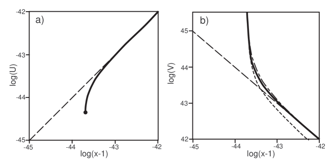
Figure 1: Dependence of the dimensionless metric functions on the dimensionless distance from the Schwarzschild sphere. Solid – numerical simulation, dotted – metric (7), dashed – Schwarzschild metric with singularity at $r_{s}$, dashed-dotted – Schwarzschild metric with singularity at $x_{1}$. Point in (a) corresponds to analytical metric (7).

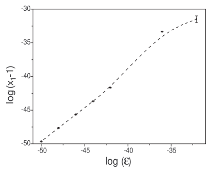
Figure 2: Distance of the singularity point from the Schwarzschild sphere depending on the dimensionless mass parameter $\epsilon$.

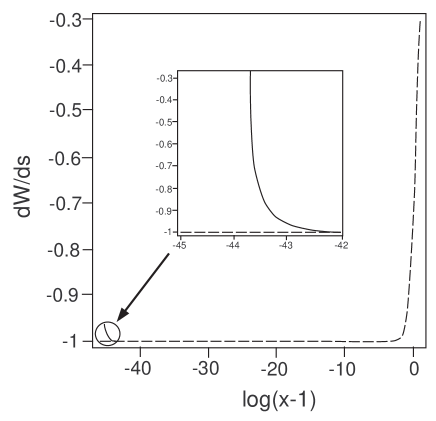
Figure 3: Velocity of the falling particle depending on the distance from the Schwarzschild sphere. Solid – numerical result from the Logunov equations, dashed – result from the Schwarzschild metric.

Firstly, we have to recognize a good accuracy of the analytical estimation in the vicinity of $x_{1}$. Note also, that the Schwarzschild solution for $V$ (dash-dotted curve in Fig. 1, b) is quite accurate if $r_{s}=x_{1}$. Secondly, the differences between Schwarzschild and Logunov metrics appear at the extremely small distance from $r_{s}$ (sub-Planckian for the stellar objects). It is clear that the latter results from the small value of $m_{g}$ and requires the quantum consideration of the Schwarzschild sphere vicinity. The dependance of $x_{1}$ on $\epsilon$ is shown in Fig. 2. One can see that the deviation of $x_{1}$ from $r_{s}$ is very small even for the extra-massive collapsars.

The approach to $x_{1}$ of the free-falling particle is described in the vicinity of the Schwarzschild sphere by the approximate expression [7]:

$$\frac{dW\left(s\right)}{ds}=-2\sqrt{\frac{x-x_{1}}{\epsilon x_{1}^{3}}},$$ (9)

which demonstrates a strong deceleration due to antigravitation induced by the massive graviton. Fig. 3 shows the numerical result obtained from Eqs. (4,8) and expression

$$\frac{dW\left(s\right)}{ds}=-\sqrt{\frac{1-U}{UV^{\ast}}}$$ (10)

for the modified interval

$$ds^{2}=U\left(W\right)dt^{2}-V^{\ast}\left(W\right)dW^{2}-W^{2}\left(d\theta^{2}+\sin^{2}\theta\ d\varphi^{2}\right).$$ (11)

One can see, that the velocity of the falling particle (for the remote observer) approaches to the velocity of light ($c=1$ in our normalization). However, in immediate proximity to $x_{1}$ the particle is decelerated by the short-range antigravitation and its velocity decreases up to zero (i.e. the Schwarzschild sphere is physically unreachable). Surely, as this deceleration takes a place at the extremely small distance, we need a quantum consideration. Nevertheless, one can suppose that the final stage of collapse can entail the over-production of the gravitons (some kind of the gravitational burst). Note also, that in spite of $x_{1}-1\ll 1$ the time of the light propagation from $r=100r_{s}$ to the point, where the deviation from the Schwarzschild metric begins, is $\approx 0.02$ s for $M=$ $10M_{\odot}$. Thus, the processes induced by the massive graviton in the vicinity of the Schwarzschild sphere are not hidden from us by the cosmological-scale time and we face the challenge of the stability of the observable massive collapsar-like objects [10].

3 Stability of the spherically symmetric metric

Although the problem of the collapsar stability can not be reduced to the stability of the metric against the small perturbation, the latter is its necessary condition. We shall base our analysis on the classical method of Ref. [11]. (7) is chosen as the perturbed metric.

The general perturbed metric has a form:

$$g_{\mu\nu}=$$ (12)

$$\begin{bmatrix}U\left(r\right),&0,&0,&\begin{array}[]{c}\begin{array}[]{c}\delta\ \omega\left(t,r,\theta\right)\times\\ W\left(r\right)^{2}\sin^{2}\theta,\end{array}\\ \end{array}\\ 0,&-V\left(r\right),&0,&\begin{array}[]{c}\begin{array}[]{c}\delta\ q_{2}\left(t,r,\theta\right)\times\\ W\left(r\right)^{2}\sin^{2}\theta,\end{array}\\ \end{array}\\ 0,&0,&-W\left(r\right)^{2},&\begin{array}[]{c}\begin{array}[]{c}\delta\ q_{3}\left(t,r,\theta\right)\times\\ W\left(r\right)^{2}\sin^{2}\theta,\end{array}\\ \end{array}\\ \begin{array}[]{c}\delta\ \omega\left(t,r,\theta\right)\times\\ W\left(r\right)^{2}\sin^{2}\theta\end{array},&\begin{array}[]{c}\delta\ q_{2}\left(t,r,\theta\right)\times\\ W\left(r\right)^{2}\sin^{2}\theta\end{array},&\begin{array}[]{c}\delta\ q_{3}\left(t,r,\theta\right)\times\\ W\left(r\right)^{2}\sin^{2}\theta\end{array},&-W\left(r\right)^{2}\sin^{2}\theta\end{bmatrix},$$

where $\delta$ is the small expansion parameter; $\omega\left(t,r,\theta\right)$, $q_{2}\left(t,r,\theta\right)$ and $q_{3}\left(t,r,\theta\right)$ are the perturbation functions.

Taking into account only linear on $\delta$ terms, using dimensionless quantities and supposing that $x_{1}=r_{s}$ and

$$\omega\left(t,r,\theta\right)=\omega\left(r,\theta\right)\exp\left(-i\sigma t\right),$$ (13)

$$q_{2}\left(t,r,\theta\right)=q_{2}\left(r,\theta\right)\exp\left(-i\sigma t\right),$$

$$q_{3}\left(t,r,\theta\right)=q_{3}\left(r,\theta\right)\exp\left(-i\sigma t\right),$$

we can obtain from (7) and second field equation (1)

$$\frac{3\cos\theta\ q_{3}\left(y,\theta\right)}{\sin\theta}-7q_{2}\left(y,\theta\right)+8q_{2}\left(y,\theta\right)\ y+2y\left(y-1\right)\frac{\partial q_{2}\left(y,\theta\right)}{\partial y}+\frac{\partial q_{3}\left(y,\theta\right)}{\partial\theta}+$$ (14)

$$\frac{2\sigma i}{\epsilon}y^{2}\omega\left(y,\theta\right)=0.$$

Eq. (14) requires $\omega\left(y,\theta\right)=0$ if $q_{2}\left(y,\theta\right)$, $q_{3}\left(y,\theta\right)$ are real and $\sigma$ is arbitrary and real. The latter requirement corresponds to the stability of the perturbed metric (7,12) in the framework of the linear stability analysis. More general consideration will be given elsewhere.

Now we consider first field Eq. (1) for the perturbed metric. The obtained expressions are too awkward to be written here and can be found in [9]. The axial perturbations are defined by the perturbed $\left(1,3\right)$ and $\left(2,3\right)$ - components of the field equations. Introducing the new function

$$Q\left(y,\theta\right)=\left[\frac{\partial q_{3}\left(y,\theta\right)}{\partial y}-\frac{\partial q_{2}\left(y,\theta\right)}{\partial\theta}\right]\sin^{3}\theta,$$ (15)

we can obtain after some manipulations (see [9]) the equations defining the perturbation functions:

$$\frac{\frac{\partial}{\partial\theta}Q\left(y,\theta\right)}{\sin^{3}\theta}=q_{2}\left(y,\theta\right)\left[2-\frac{6}{y}+\frac{2y^{2}\sigma^{2}}{\epsilon}-4\epsilon y^{2}\Delta\left(y\right)\right],$$ (16)

$$\frac{\frac{\partial}{\partial y}\left(\Delta\left(y\right)Q\left(y,\theta\right)^{2}y^{2}\right)}{Q\left(y,\theta\right)\ y\sin^{3}\theta}=2q_{3}\left(y,\theta\right)\ y^{3}\left[\frac{\sigma^{2}}{\epsilon}-\epsilon\sin^{2}\theta\right],$$

where $\Delta\left(y\right)\equiv y^{2}\left(1-\frac{1}{y}\right)$. Now it is possible to eliminate $q_{2}$ and $q_{3}$. This results in

$$\frac{\partial}{\partial y}\left[\frac{\frac{\partial}{\partial y}\left(\Delta\left(y\right)Q\left(y,\theta\right)^{2}y^{2}\right)}{Q\left(y,\theta\right)\ y\ \sin^{3}\theta\ B\left(y\right)}\right]+\frac{\partial}{\partial\theta}\left[\frac{\frac{\partial}{\partial\theta}Q\left(y,\theta\right)}{\sin^{3}\theta\ A\left(y\right)}\right]=\frac{Q\left(y,\theta\right)}{\sin^{3}\theta}.$$ (17)

Here $A\left(y\right)=-2+\frac{6}{y}-\frac{2y^{2}\sigma^{2}}{\epsilon}$, $B\left(y\right)=$ $-\frac{2y^{3}\sigma^{2}}{\epsilon}$ and we used the smallness of $\epsilon$ in order to eliminate the angular-dependence from $A$ and $B$.

Eq. (17) permits the separation of variables: $Q\left(y,\theta\right)\equiv\Xi\left(y\right)\Psi\left(\theta\right)$. Then for the angular part we have the Gegenbauer’s equation:

$$\frac{d^{2}}{d\theta^{2}}\Psi\left(\theta\right)-3\frac{\cos\theta}{\sin\theta}\frac{d}{d\theta}\Psi\left(\theta\right)+2n\Psi\left(\theta\right)=0,$$ (18)

where $n$ is some number. Eq. (18) can be solved through Legendre functions and then

$$n=\frac{\left(l+2\right)\left(l-1\right)}{2},$$ (19)

$l$ is integer.

Taking into account that $\epsilon\ll 1$, the equation for the radial part is

$$2\epsilon y\Delta\left(y\right)\frac{d^{2}}{dy^{2}}\Xi\left(y\right)+\epsilon y\left(4y-1\right)\frac{d}{dy}\Xi\left(y\right)+$$ (20)

$$2\Xi\left(y\right)\left[\sigma^{2}y^{3}-\epsilon yn-2\epsilon y+3\epsilon\right]=0.$$

In immediate proximity to the Schwarzschild sphere and outside the $\Xi\left(y\right)$-extremum (which appears as a result of the angular number growth, see below Eq. (21)), we can neglect the first term in Eq. (20). Hence, the approximate solution of Eq. (20) is:

$$\Xi\left(\lambda\right)\approx C\left(1+\epsilon\lambda\right)^{6}\left(3+4\epsilon\lambda\right)^{\left(-\sigma^{2}+16\epsilon\left(n-10\right)\right)\diagup 32\epsilon}\exp\left[-\frac{\sigma^{2}\left(1+\epsilon\lambda\right)\left(3+2\epsilon\lambda\right)}{8\epsilon}\right],$$ (21)

where $C$ is the constant of integration and $\lambda>0$: $y\equiv 1+\epsilon\lambda$.

Eq. (21) suggests that the appropriate asymptotic for $\Xi$ is provided only by $\sigma^{2}>0$. Thus, the perturbation increment $\sigma$ is real in the agreement with the stability requirement. The stability far from $x_{1}$, where the metric coincides with the Schwarzschild one, is provided by the stability of the latter.

4 Conclusion

The numerical simulations based on the Logunov field equations demonstrate a high accuracy of the approximate analytical solution for the static spherically symmetric metric in the RTG. It is shown, that there exists a strong repulsion induced by the massive graviton at the Planckian distance. As a result of this repulsion, the collapse of the stellar objects has to entail the burst of the gravitational radiation. However, the rigorous analysis of the collapse requires taking into account the quantum effects. Some case for the stability of the collapsar is provided by the stability of the static spherically symmetric metric.

As the outlooks for the future analysis we can point out the following topics: i) more general stability analysis including higher-order perturbations; ii) classical consideration of the possible static configurations of the matter in the static spherically symmetric metric; iii) realistic collapse models taking into account the energy loss due to gravitational radiation in the vicinity of the Schwarzschild sphere.

References

• [1] A.A.Logunov, “Relativistic theory of gravity”, Nova Sc. Publ., 1998.
• [2] A.A.Logunov, M.A.Mestvirishvili, “Relativistic theory of gravitation”, Nauka, Moskow, 1989 (in russian).
• [3] A.A.Logunov, “The theory of gravitational field”, Nauka, Moskow, 2000 (in russian).
• [4] A.A.Logunov, “The theory of gravity”, arXiv:gr-qc/0210005.
• [5] S.S.Gerstein, A.A.Logunov, M.M.Mestvirishvili, “Graviton mass and total relative density of mass $\Omega_{tot}$ in Universe”, arXiv:astro-ph/0302412.
• [6] V.L.Kalashnikov, “Quintessential cosmological scenarious in the relativistic theory of gravitation”, arXiv:gr-qc/0208070.
• [7] A.A.Logunov, M.A.Mestvirishvili, “What happens in the vicinity of the Schwarzschild sphere when nonzero gravitation rest mass is present”, arXiv:gr-qc/9907021.
• [8] the detailed development of this system can be found in [7] and is realized as Maple 8 computer algebra algorithm in http://www.geocities.com/optomaplev/programs/rtg_bh.html.
• [9] V.L.Kalashnikov, “Spherically symmetric collapsar in the relativistic theory of gravitation”, http://www.geocities.com/optomaplev/programs/rtg_bh.html.
• [10] P. Charles, “Black holes in our Galaxy: observations”, arXiv:astro-ph/9806217; Y. Tanaka, “Observation of black holes in X-ray binaries”, in Proc. IAU Symp., v. 195, p.37 (2000).
• [11] S.Chandrasekhar, “The mathematical theory of black holes”, Clarendon Press, 1983.