GOTPM: A Parallel Hybrid Particle-Mesh Treecode

Abstract

We describe a parallel, cosmological N-body code based on a hybrid scheme using the particle-mesh (PM) and Barnes-Hut (BH) oct-tree algorithm. We call the algorithm GOTPM for Grid-of-Oct-Trees-Particle-Mesh. The code is parallelized using the Message Passing Interface (MPI) library and is optimized to run on Beowulf clusters as well as symmetric multi-processors. The gravitational potential is determined on a mesh using a standard PM method with particle forces determined through interpolation. The softened PM force is corrected for short range interactions using a grid of localized BH trees throughout the entire simulation volume in a completely analogous way to P³M methods. This method makes no assumptions about the local density for short range force corrections and so is consistent with the results of the P³M method in the limit that the treecode opening angle parameter, $\theta\rightarrow 0$.

The PM method is parallelized using one-dimensional slice domain decomposition. Particles are distributed in slices of equal width to allow mass assignment onto mesh points. The Fourier transforms in the PM method are done in parallel using the MPI implementation of the FFTW package. Parallelization for the tree force corrections is achieved again using one-dimensional slices but the width of each slice is allowed to vary according to the amount of computational work required by the particles within each slice to achieve load balance. The tree force corrections dominate the computational load and so imbalances in the PM density assignment step do not impact the overall load balance and performance significantly. The code performance scales well to 128 processors and is significantly better than competing methods. We present preliminary results from simulations run on different platforms containing up to $N=1G$ particles to verify the code.

, , , and

1 Introduction

As we enter the era of precision cosmology, the need for higher resolution cosmological simulations has never been clearer. Recent determinations of the cosmological parameters to accuracies of a few percent by the WMAP mission (Bennett et al 2003) will entirely transform the industry of cosmological N-body simulations. Since the initial conditions are now well-defined, the focus will be on seeking detailed quantitative consistency with the prevailing cosmological paradigm with observations of the large-scale structure through clustering and lensing studies and detailed analysis of the structure and dynamics of galaxy clusters and galaxies themselves. During the last decade, there has been a huge growth in computational power brought on by steady increase in processor speed and the integration of processors into massively parallel architectures. Numerical cosmologists and dynamicists have developed parallel, N-body codes to take advantage these architectures and there are now a variety of codes that are being used to simulate the formation of large-scale structure and galaxies. In this paper, we describe a new parallel code that is adaptable and scalable to the next generation of parallel supercomputers.

Two classes of cosmological N-body codes are now used widely and are based on either the Particle-Mesh (PM) algorithm (Hockney and Eastwood 1981) or the Barnes-Hut Tree algorithm (1986). PM codes are the fastest available taking advantage of the fast Fourier transform algorithm (FFT) to solve Poisson’s equation. While useful for some cosmological applications, pure PM codes fail to resolve structures on scales smaller than the mesh size. Different approaches have been taken increase the force resolution on the sub-mesh scale. The simplest approach is the P³M algorithm where the mesh softened force is corrected at short range using direct summation of pairwise forces between particles (e.g. Hockney and Eastwood 1981, Efstathiou et al 1985). As systems become clustered, the P³M algorithm scales as O(N${}_{h}^{2}$) where N_h is the size of the largest halos limiting its application to small N or very large cosmological volumes where halos contain modest numbers of particles. Another approach is to lay down refined sub-meshes on regions of high density to compute force refinements. This can be done hierarchically and leads to accurate force determination and code speed up. Couchman’s (1991) AP³M algorithm used in the Hydra code has been highly successful. A slight disadvantage of this approach is that a density threshold criterion is necessary to lay down sub-meshes and there may be discrete changes in force resolution across arbitrarily set boundaries that have unpredictable effects. An alternative mesh-refinement scheme is provided by Kravtsov et al. (1997) in the ART algorithm that lays down refined meshes as particles begin to crowd into mesh cells. A completely different approach uses the BH tree algorithm modified to include periodic boundary conditions using Ewald’s method (Bouchet, Hernquist and Suto 1991). This method has the advantage that forces are accurately determined at all stages of the calculation on all scales. The penalty is that tree codes generally have much larger memory requirements and require significantly more computation to achieve a similar force accuracy than PM based algorithms. Despite these problems, tree codes based on Ewald’s method have been easier to parallelize then AP³M are currently very competitive in many applications (e.g. Davé et al 199?, Springel et al. 2001).

A natural evolution of cosmological codes is the developments of hybrids that can incorporate the high efficiency of PM codes for long range force determination and the advantage of tree codes for short range force corrections. Xu (1995) developed a hybrid Tree/PM (TPM) algorithm that is in the spirit of AP³M and the algorithm has since been enhanced by Bode et al. (2000). BH trees are used in place of refining sub-meshes and constructed around dense clustered regions to determine short range force corrections. This method differs from the Ewald-method treecodes in that short range forces drop to zero at a few mesh lengths so trees only need to be built locally to calculate the force corrections. The algorithm has also been parallelized and is scalable to large processor numbers (e.g. Bode and Ostriker 2003). Bagla has also introduced a hybrid TREEPM algorithm that breaks the forces up into short and a long range parts using Ewald’s original formalism. The main difference from TPM is that short range forces are corrected using the BH tree method throughout the simulation volume with no need to specify a density threshold for laying down a tree.

In this paper, we describe a new Tree/PM hybrid that is in the same spirit as Bagla’s method but with parallelization. We call this new algorithm GOTPM standing for Grid-of-Oct-Trees-Particle-Mesh. In §2, we describe the details of the algorithm including a new parallel PM method based on the FFTW fast Fourier transform package (Frigo et al. 1998) and a method for computing the force refinements using localized BH trees. Since tree refinements are confined to a few mesh lengths, the process of building trees within the simulation volume can be done sequentially leading to large savings in memory compared with Ewald tree codes. We also discuss how to load balance the short range force correction calculations. In §3, we present measures of the force accuracy and timing tests on a variety of machines to measure the code’s performance and parallel scalability. In §4, we describe some preliminary results of various simulations with the largest containing N=$1024^{3}$ particles. In §5, we discuss the future incorporation of multi-timestepping and smoothed particle hydrodynamics and algorithmic improvements that will permit simulations containing $N=8-64G$ particles on next generation parallel machines.

2 Parallel TREEPM

2.1 Parallel PM

The PM algorithm is well documented so we highlight here the features of our implementation and method of parallelization. We use the PM code developed by Park (1990, 1997) as our starting point and it follows the usual steps:

1. We determine a density field on a mesh from the particle distribution using the triangular-shaped cloud (TSC) mass assignment scheme.

2. A Fast Fourier transform (FFT) of the density field is calculated and then multiplied by the appropriate Green’s function for the TSC scheme to determine the transform of the potential field.

3. An inverse FFT determines the potential field in real space.

4. We interpolate the potential field to determine the gravitational force at each particle position using a 4-point finite difference approximation (FDA).

We have parallelized this algorithm using a simple, slab domain decomposition of the simulation cube using the Message-Passing Interface (MPI) library. Particles are first distributed in slabs of equal width with an integral number of mesh divisions. We determine the density field using the TSC method in each slab in each processor. Since the TSC method weights the particle mass to each of the surrounding 27 grid points from the nearest grid point, we need to communicate the contribution to the density field from particles near the boundaries of the slabs. We achieve this by binning the mass on ghost slices of mesh that are communicated to their neighbours and summed on to the corresponding local slices to find the correct density field quantities.

Once the density fields on slabs in each processor are determined we then use the FFTW library (Frigo et al. 1998) with MPI extensions to calculate the FFTs used to obtain the gravitational potential. The FFTW package requires that the complete mesh be divided in slabs of equal width so we can determine the gravitational potential immediately with a parallel FFT. With the potential, we then calculate the particle forces in each slab using FDA interpolation. Again, we need to import images of mesh slices at the boundaries to determine forces on particles. We communicate the 3 or 4 mesh slices from the front and back sides of the slab and then calculate the force on each particle in each processor in parallel. Our implementation assumes all neighbouring mesh slices are in adjacent slabs so the slab width can be no smaller than 4 mesh divisions. This sets a limits on the number of processors that can be used in a parallel run e.g. only 128 processors can be used with a $512^{3}$ mesh. Although the code will work with thin slabs, we find in practice below that problems can arise with memory imbalance in the tree algorithm if slices are too thin so slabs with more than 8 mesh divisions are preferred.

2.2 Force Shaping

In the complete algorithm, we treat the PM force as the long range contribution to the total force and determine the short range contribution using the tree algorithm. The PM method softens the Newtonian potential within a few mesh divisions and also introduces some anisotropy to the force on the mesh size scale. We follow the lead of other codes and smooth the PM potential using a Gaussian filter with an e-folding radius of 0.9 times the mesh size. To characterize the resultant PM force, we calculate the force many times at a point from a single particle placed at random positions within the mesh in a otherwise homogeneous density field. Figure 1 shows usual behaviour with an asymptotic Newtonian force with significant scatter due to anisotropy at the maximum around $r=1.4\Delta x$ where $\Delta x$ is the mesh cell size. Our strategy is to fit these points with a smooth function of radius which asymptotically behaves as $1/r^{2}$ with a best fit shown in Figure 1. After some experimentation, we settled on the rather complex fitting function,

$$\begin{array}[]{ll}F(x)=&a\tanh(bx)/x^{2}-ab/(x\cosh^{2}(bx))\\ &+cx(1+dx^{2})\exp(dx^{2})\\ &+e(1+fx^{2}+gx^{4})\exp(hx^{2}),\end{array}$$ (4)

and find it successfully fits the data. The short range force is simply determined as the difference between this smooth empirical function and the Newtonian gravitational force. We also determined the scatter in the expected relative force error by laying down a single particle randomly within the grid and measuring the acceleration due to the mesh plus correction at random points. Figure 2 show that the scatter peaks at a separation of about 2 mesh cell sizes revealing the anisotropy introduced by working on a regular cubic mesh. These errors are intrinsic to PM methods and we see below in more general situations they introduce a tail in the acceleration error distribution in the 1-2% range.

Figure 1: The PM force is calculated in a $N_{mesh}=256$ box at arbitrary positions around a randomly positioned test particle in a homogeneous background and plotted revealing the scatter due to force anisotropies imposed by the mesh. The solid line is the best fit to the PM force according to our fitting function. The force is normalized for unit mass and plotted versus the separation in mesh cell sizes. The dashed line represents the ideal Newtonian force that adaptive refinements try to achieve.

Figure 2: Scatter in the relative error in the mesh force + short range correction force versus separation in mesh units at randomly distributed points from a randomly distributed point mass. Anisotropies in the mesh force lead to a large scatter at the mesh scale.

2.3 Correcting Forces with BH Trees

The parallel PM force is very efficient at determining long range gravitational forces but because of the finite mesh size the forces from nearby particles are highly softened. The standard way to overcome this deficiency is to define a new correction force law for local particles that is the difference between the desired Newtonian force and the force law determined by the PM method, $F_{c}=F_{N}-F_{PM}$. The correction force has the property that it is nearly Newtonian on the sub-mesh scales but then falls to zero beyond four mesh cell sizes where the PM forces become nearly Newtonian. The gravitational potential is also softened using a Plummer law on the subgrid scale. We typically use a softening radius of $5\times 10^{-5}L$, where L is the boxsize i.e. so typical simulations are equivalent in resolution to a PM method with a $20000^{3}$ mesh.

Three approaches have been used to determine $F_{c}$ in PM methods. Direct force evaluation using the particle-particle (P²) method (Hockney and Eastwood 1981), adaptive particle sub-meshes with P²(Couchman 1991), and tree methods (Xu 1995, Bode et al. 2000, and Bagla 2000). Direct force evaluation is the most general method and is easily parallelizable. Unfortunately, when clustering is strong the method grinds to a halt because of the $O(N^{2})$ nature of the method. Couchman’s (AP³M) method relies on laying a local refined mesh on regions where strong clustering is occuring and calculating correction forces from this sub-mesh. It is highly efficient in serial codes but has proved difficult to parallelize. Finally, Xu’s hybrid TPM algorithm works in a similar way to AP³M but a Barnes-Hut tree is built locally on clustered regions. This method has been parallelized and performs well (e.g. Bode et al. 2003). A disadvantage of both these methods is that one requires an arbitrary criterion to establish whether a mesh volume contains clustered material that should be refined. Furthermore, boundaries between finely resolved and more coarsely resolved volumes are sharp and it is not clear if there are physical consequences to assigning these boundaries.

Bagla (2000) provides a way to characterize both the short and long range forces in his TREEPM algorithim and is completely analogous to P³M in that all local forces everywhere within the volume are corrected. We describe here a parallel version of this method that builds on the parallel PM algorithm above and incorporates most of the efficient tree-building and tree walking software of Dubinski’s (1996) parallel tree code PARTREE. We call our new parallel algorithm GOTPM for Grid of-Oct-Trees-Particle-Mesh. This new code has the generality of a $P^{3}M$ code in that all forces throughout the simulation volume are calculated accurately on the submesh scale with no density criteria imposed for the addition of refinement. The equivalent of mesh refinement is done automatically by building trees everywhere within the simulation volume at every step. We show below that this algorithm also is easy to load balance using algorithms taken from pure parallel tree codes.

2.4 GOTPM: A New Tree/PM Hybrid Algorithm

It is easiest to describe this algorithm by comparing it directly to the P³M method. The $P^{2}$ correction force on a particle is determined by summing directly over particles within a sphere centred on the particle which extends out to 2-3 mesh cell sizes. Beyond this boundary corrections on the mesh force are small, generally less than 1%, and are so neglected. The problem with $P^{2}$ correction, however, is that the algorithm scales inherently as $O(N_{h}^{2})$ and a code is therefore slowed down considerably when clustering occurs. In constrast, the tree algorithm is $O(N\log N)$ and generally requires about 2 to 3 times the amount of work when going from a homogeneous to a clustered state.

The strategy we employ is to replace $P^{2}$ force correction with a correction determined by the tree method. The details of the basic BH tree method as implemented here are presented in Dubinski (1996) with the only difference being that the force law is given as the difference between the Newtonian and PM force law given in equation (1). In brief, the BH tree algorithm works by arranging particles in a hierarchy of cubes or cells in an oct-tree structure. Forces are determined by descending the tree and summing contributions from interactions with distributions of particles in “distant” cells and nearby particles. Cell interactions are determined from the quadrupole order expansion of the potential of the particles within the cube rather than through direct summation so there are great computational savings. The trick is to introduce a cell opening criterion based on the ratio of the size of a cube to the distance of its centre of mass, i.e. an opening angle. If the cell is big and nearby, then the opening criterion is satisfied such that the cell is broken down into its 8 sub-cells each of which is examined in turn. If the cell is small and sufficiently distant, the opening criterion fails and the quadrupole order expansion of the particles in the cell are used to determine the force and the tree descent ends at this node. In practice the tree method requires only $O(N\log N)$ computations per step to determine forces with an error of 1% and therefore has a great advantage over direct summation methods. There are different choices available for the cell opening criterion as well as strategies for grouping particles to minimize the overhead in tree walks. The cell opening criterion and grouping strategy we use here is the same as that described in Dubinski (1996) with some slight modifications that we discuss below.

The application of the tree method to determine force corrections in a PM code requires a few general modifications. The force correction effectively drops to zero at a few mesh lengths. It is therefore not necessary to build a global tree for the entire particle distribution in the simulation cube. Since the forces are localized, we can build a grid of trees, with a dimension of a few mesh lengths. If we define $R_{max}$ as the radius where the correction forces drops to small fraction of a percent then we only need to calculate the contributions from particles within this radius. In P³M, one generally sets $R_{max}=2\sim 3$ but we find in practice for the tree algorithm that $R_{max}=4$ is necessary to assure accuracy. This scale is set to the length of the cubes enclosing the trees. Each particle is incorporated into one tree so to determine the force correction on a particle we need only descend the particle’s home tree and the surrounding 26 trees (Figure 3).

Figure 3: Schematic diagram of the implementation of short range tree forces in GOTPM. In a P³M algorithm, the short range force is determined through direct summation of forces on particles within a sphere with radius $R_{max}$. In GOTPM, particles are binned in cubes of width $R_{max}$ and Barne-Hut trees are constructed from the binned particles with a tree for each cube. Short range forces are determined by walking through the particle’s home tree and surrounding 26 trees in 3D. A spherical boundary is not required for large enough values of $R_{max}$ since the contribution from distance cells becomes small. In practice, we need to use $R_{max}=4\Delta x$ where $\Delta x$ is the mesh division.

In principle, P² force corrections are necessary from all particles within the volume although particles beyond $R_{max}$ contribute little to the correction. In practice, particles beyond $R_{max}$ are simply ignored saving a lot of time. This is necessary since the number of particles surrounding the point where the potential is calculated grows rapidly with radius i.e. $N\sim r^{3}$ for a homogeneous system and $N\sim r$ when clusters with densities of $\rho\sim r^{-2}$ develop. In a tree code, however, the number of interactions does not grow rapidly with radius. Distant particles are grouped into larger and larger cells so the number of cell interactions only grows roughly as $N\propto\log r$ under most circumstances. It is therefore not necessary to impose a hard spherical boundary of $R_{max}$ as is done in the $P^{3}M$ method. As long as the trees are $R_{max}$ in size then all effective contributions to the force correction will be accounted for and the extra forces from the irregular jagged region beyond the spherical boundary will be small and generally average out. The force corrections themselves will have an inherent error which depends on the value of the critical opening angle in the tree algorithm and the value of $R_{max}$. In practice, we show below that as clustering develops the number of particle cell interactions only grows slowly from the initial homogeneous state to the strongly clustered regime. Computationally, the CPU time per step only grows by a factor of three from the beginning to the end of a simulation.

Since the trees are localized and compact there is one further refinement that can be added to improve accuracy and efficiency. If the number of particles within a cube is small, the cost of building and walking the tree for force determinations can be greater than simply doing a direct forces summation. We introduce an additional parameter, $N_{tree}$, that defines the minimum number of particles required for a tree build. If the number of particles in a bin is less than $N_{tree}$ then we do a direct P² summation for all particles within the radius $R_{max}$. Otherwise, we use the tree machinery for the force calculation. In this mode, a typical run behaves as a P³M code at early times while at late times trees are used to calculate forces wherever clusters develop.

Since force corrections are local, we see that this algorithm is easily parallelizable within the context of the PM code we have described. We outline the implementation of this algorithm below.

2.5 Slice domain decomposition

The parallel PM code we describe above distributes the particles into domain slabs of equal width and assigns them to independent processors on a parallel computer. We retain this slab domain decomposition scheme for force corrections with trees but relax the constraint of equal widths for the slices to achieve better load balance. As the system evolves, particles cross these boundaries and must be moved between processors by exchanging messages.

The inner loop of the algorithm is as follows:

1. Particles are redistributed into domain slices of equal width by exchanging messages for the next PM force evaluation.

2. The PM force is determined using the slice domain decomposition parallel method described above.

3. Particles are now redistributed into slices of variable width such that the amount of treecode computation per slice is equal. The boundaries of these domains are determined iteratively using the number of tree force interactions from the last step. It is a one-dimensional version of the orthogonal recursive bisection (ORB) domain decomposition method described in Dubinski (1996) and used in other parallel tree codes like GADGET (Springel et al. 2001). At the end of this step, each processor contains a list of particles which requires the same amount of computation to determine tree force corrections.

4. We are now ready to build a local grid of trees for the force correction. To do this, we need to import “ghost” particles from neighbouring domains extending a distance $R_{max}$ from the current slice boundaries. This is accomplished by exchanging particles with neighbouring processors. These ghost particles along with the local particles are then binned into cubes of dimension $R_{max}$ in the slice. To save memory, we only import the positions (and masses if variable masses are present) for the ghost particles.

5. For each particle bin, we then build a BH tree.

6. We now loop through the local particle list determining the force correction using tree descents from the surrounding 27 trees centred on each particle. We remember the number of interactions required for each particle for load balancing purposes in step 3 above.

7. Force corrections are now added to the PM force to determine the corrected Newtonian force in a periodic universe.

8. Particles are pushed forward according to the equations of motion and a leapfrog integration scheme.

Figure 4 illustrates the domain decomposition scheme needed for the FFT’s and achieve load balance for short range tree forces.

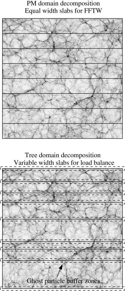
Figure 4: Two modes of slab domain decomposition required to compute PM long range forces and tree short range force corrections. The PM method requires particles binned in slabs of equal width for mass assignment and the use of FFTW to compute the potential. The tree method requires variable width domains for computational load balance. The width of domains is determined by the equalizing the computational load as measured by the number of particle interactions in each slab using a recursive bisection technique. Ghost particles from buffer zones of width $R_{max}$ on each side of a slab are imported to build boundary trees. The periodic boundaries are also implemented by importing trees from opposite sides of the cube where appropriate.

There are a few refinements to this algorithm that improve speed and minimize memory overhead. First, step 3 is generally expensive in terms of communication time since the domain boundaries must be determined iteratively in $\log_{2}N_{proc}$ message exchanges each possibly requiring the communication of large numbers of particles. To speed this step up, the full ORB decomposition is only done every 10 steps. At intermediate steps the boundaries are held fixed according to the last determination. Since the system does not change dramatically from step to step, only a small fraction of the particles actually cross these boundaries between steps thereby minimizing communication and preserving load balance. Second, we save on memory when building the trees in steps 5 and 6 by only building a small subset of the trees at a time and discarding them after we are done with them. Tree structures inherently require large amounts of data to describe the relational aspects of the tree through pointers and the cells themselves require lots of extra information including the quadrupole components as well as cell dimensional information. Since all force corrections for a particle are local to the surrounding 27 trees, we can build the trees in small groups, determine the correction forces for corresponding particles then discard the trees before building a new set. In practice, we build only $8\times 8\times n_{z}$ grid columns of trees and loop through the volume where $n_{z}$ is the number of trees in the vertical direction. The slice height $n_{z}$ varies from step to step because of the domain decomposition. For example, in a typical simulation on a 32 processor machine with a $1024^{3}$ mesh with $R_{max}=4.0$, there are on average $256\times 256\times 8=512K$ trees that need to be built in each processor. We only need to build 512 trees at a time with this method saving a factor of 1000 in memory for tree data structures. The only information one needs to save at each step is the basic particle data, i.e. positions, velocities, particle index and computational load. Extra memory is required to handle neighbour particles and memory imbalance induced by the load-balancing algorithm itself. For small cosmological volumes with a great deal of clustering, the memory imbalance leads to roughly a factor of 2 variation in the number of particles per processor. In the worst case, we require about 3 times the memory required for basic particle data (masses, positions and accelerations) to handle this problem.

2.6 Memory budget

The memory budget for a pure n-body simulation can be broken down into particle memory and mesh memory. A typical mesh requires $4\times N_{mesh}^{3}$ bytes for single precision and twice that for double precision. The particles themselves require memory for positions, velocities, accelerations, masses and softening lengths, a computational work measurement, a particle index to retain identity and a pointer for constructing linked lists when binning particles in cubes. The total budget is the equivalent of 56 bytes per particle in single precision or 112 bytes in double precision. Because of imbalance in particle numbers in the domain slabs the worst case that occurs with the smallest box sizes leads to domains with up to 3 times the average number of particles. Conservatively, approximately 150 bytes are required per particle in a typical single precision run. The ghost particles can potentially eat up significant amounts of memory when the domain slabs become thin. This deficiency can be removed in future versions by using fully 3-D domain decomposition in the tree correction phase though considerable bandwidth may be required to move particles back and forth from slabs in the PM phase and cuboids in the tree phase.

In summary, a typical run with $N_{mesh}=2048^{3}$ and $N_{p}=1024^{3}$ requires $\sim$200 GB in single precision in the worst case of a small box. This new algorithm is considerably more memory efficient than pure cosmological treecodes that require lots of memory to describe global trees.

3 Code Verification

3.1 Accuracy Tests

To validate the correctness and accuracy of the code, we calculated the accelerations from a 2M particle dark matter simulation in a $50h^{-1}$ Mpc box at $z=0$ in a standard cosmology with $\Omega=0.3$ and $\Lambda=0.7$. This resulting particle distribution is strongly clustered and so represented a good test for the method’s accuracy. We used several methods to measure the accelerations. To start, we used a cosmological parallel treecode based on the Ewald method (Davé et al. 1997) to determine accelerations with small errors by setting the opening angle parameter $\theta=0.1$ and computing cell-particles interactions to quadrupole order. We used a Plummer softening length of $5\times 10^{-5}$ times the box size. This is a costly calculation but the mean relative error in the accelerations $|\delta a/a|$ is estimated to be $<0.01$%. We consider these accelerations to be exact for the purpose of comparison to other methods. We then calculated acceleration errors using the Ewald method with a more standard value of $\theta=0.8$ and the new GOTPM algorithm with $\theta=0.0$ (making it a $P^{3}M$ method) and $\theta=1.0$ with $N_{tree}=4$ and 32. The size of the mesh is $256^{3}$. In the GOTPM algorithm, we expect errors to arise both from the treecode approximation as well as the PM method itself. The technique of fitting a smooth potential to the PM force function minimizes but does not eliminate errors induced by close range anisotropies in the mesh force.

Figure 5 shows the distribution of relative acceleration errors for various methods and parameter combinations. The first result is that the values of accelerations between the Ewald-tree method and GOTPM algorithm agree with each other on the percent level. This result reassures us that the computed accelerations are physically correct since the two numerical methods are very different in their mathematical formulation: the first method is based on a combination of the Ewald expansion of a periodic point mass potential and the second method based on the solution of Poisson’s equation using Fourier methods. We can clearly see the convergence to smaller errors when going from the P³M to GOTPM method with $\theta=1.0$ and smaller values of $N_{tree}$. The distribution of errors in the P³M represents the “best” one can do to reduce errors in the accelerations using a hybrid PM method of this form. The distribution of errors between the P³M method and GOTPM methods are almost indistinguishable when $N_{tree}=32$ while the time taken to compute these forces using P³M requires about 10 times as much CPU time. For larger N simulations, the discrepancy in CPU time becomes even greater. The distribution of errors for a Ewald-method treecode using a typical value of $\theta=0.8$. Although, the mean error is slightly less than the GOTPM method there is a broader tail in the distribution to larger errors precluding the use of a larger value of $\theta$. The Ewald-method treecode method requires about 3 times as much CPU time to compute accelerations of comparable accuracy to the GOTPM method in the clustered state. We note, however, the situation is very different when the systems are less clustered. The GOTPM method is several times faster and more accurate when the system is less clustered since it operates essentially like a pure PM method. In constrast, the Ewald tree method is only slightly faster in the less clustered case and acceleration errors tend to be much larger for a given value of $\theta$.

Using a larger mesh size also increases the accuracies of the accelerations and as we see below can also requires less computation so if enough memory exists it can be advantageous to use a finer mesh for the PM part of the calculation.

Also apparent is a tail of the distribution of errors that remains as $\theta$ decreases. The cause of this tail is due to the anisotropy of the PM force on the mesh scale which introduces a random error on the determined acceleration for particles. This error is inherent to the PM method itself and all techniques using meshes will have this problem. We also note that the acceleration can be near zero because of the periodic nature of the force so relative errors are amplified in this case and do not necessarily indicate low accuracy. A plot of the acceleration versus the relative error indeed shows that the largest acceleration errors occur for the smallest accelerations. For $\theta=1$, the acceleration errors are found to be $0.43\%\pm 0.56\%$, the range typically tolerated in treecode simulations. There does not seem to be a large gain in accuracy in going to smaller $\theta$ because of mesh-induced force errors. All methods base on PM forces plus correction will have these errors so we recommend using $\theta=1$ as a compromise between speed and accuracy since generally 0.5% errors are usually tolerated in collisionless n-body calculations. We note, however, that the relative errors are much smaller for particles feeling large accelerations in the centre of clusters in these simulations so the 0.5% error is a conservative estimate.

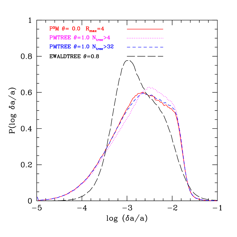
Figure 5: Distribution of relative errors in particle accelerations for a clustered 2M particle CDM simulation at z=0 ($\Omega_{m}=0.3$, $\Lambda=0.7$, $L=50$ h^-1 Mpc for P³M, GOTPM and a Ewald-method cosmological treecode. The GOTPM code with $\theta=1$ and $N_{tree}=32$ results in errors similar to P³M and comparable to treecodes while using much less computing time.

3.2 Code Performance

The GOTPM code has been run on a variety platforms including a 32 processor IBM SP3 in Seoul, an HP/Compaq GS320 and a Beowulf cluster based on Intel Xeon 2.4 GHz chips with gigabit networking both at CITA. We present results of the code performance and parallel scaling up to 128 CPUS on the Beowulf cluster though runs with up to 256 CPUS have been done and perform well. Our reference simulation computes the evolution of $N=256^{3}$ particles using a $512^{3}$ mesh in a 200 h^-1 Mpc box in a standard cosmology with $\Omega_{m}=0.3$ and $\Lambda=0.7$.

To study scaling of the code speed with processor number, we follow the computation for 5 equal time steps from $z=1$ when the system is moderately clustered and time the PM and tree phase of the code separately to determine a speed. These timing tests are done on a Beowulf cluster with gigabit networking and dual Xeon 2.4 GHz processors with code compiled using the Intel C and Fortran compilers. Figure 6 shows the code speed versus the number of processors $N_{p}$ from 4 to 128 processors. The speed scaling is not perfect since the amount of communication time grows as $N_{p}$ increases. As $N_{p}$ grows, the domain slabs become thinner and the number of particles crossing boundaries through both particle redistribution for load-balancing purposes grows significantly as well as the number of ghost particles imported for tree builds. Nevertheless, the code scales well to $N_{p}=128$ requiring only 11.6 second per step and clocking at about 1.4 million particles/s. The PM portion of the calculation only requires 1.8 seconds compared with 9.8 seconds for the tree correction force so the code is dominated by determination of the short range forces.

As part of J. Kim’s doctoral work, we simulated $1024^{3}$ particles in LCDM and SCDM cosmological models in a cosmological box of size $L=512h^{-1}$ Mpc. The simulations were run on a IBM SP3 (Regatta) system at the Korea Institute of Science and Technology Information (KISTI). Over the course of two months, we used one node of 32 CPU’s with 208 Gbytes of memory for two GOTPM simulations. Memory limited us to a $1024^{3}$ mesh. Each model was simulated with 460 time steps in 16 wall-clock days and the peak memory usage was about 170 Giga bytes. The simulation details will be presented in Kim’s thesis and a forthcoming publication. The CPU timing of the LCDM simulation is displayed in Figure 7. The CPU time per step grew from 40 minutes to 55 minutes largely due to the increase of tree calculation overload caused by the clustering of particles. Periodic spikes in DD and the total CPU time plot are due to the particle backup at every 15 time steps and pre-halo finding calculations every 5 time steps. The increase of CPU time in the FDA part was partially due to the steady increasing rates of cache miss of particle data in L2 cache. As the system evolves, the memory locality of the particle data differs significantly from the spatial positions of the particles. In Figure 8, we show the inhomogeneity of particle distributions of PM domain slabs in the LCDM simulation. We expect the density fluctuation$\Delta(r)$ at length scale $r$ is related to the power index $n$ as (Longair 1998)

$$\Delta(r)=\left({r\over{8h^{-1}{\rm Mpc}}}\right)^{-{n+3\over 2}},$$ (5)

where $r$ is defined to be the radius of a sphere having equal volume of the local domain slab. In the case of $n=-1,-2$, $\Delta(M)$ of the simulation domain slabs is $0.16,0.03$, respectively. Hence the static domain decomposition of the PM part does not matter seriously to memory budget overload for cosmological volume.

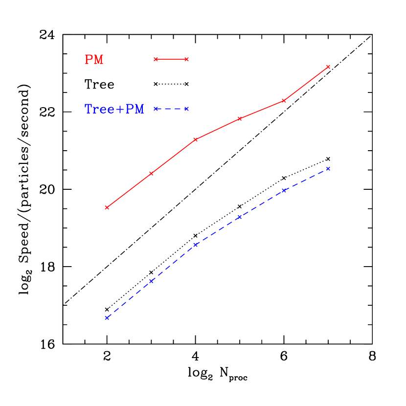
Figure 6: Code speed measured in particles per second versus number of processors for a $N=256^{3}$ particle CDM simulation in a $512^{3}$ mesh with moderate clustering. The code scales well to 128 processors and the bulk of computing time going into short range force calculations using the tree method.

Figure 7: CPU time per step in a 1G particle simulation. Only cpu times of important parts in the code are displayed; FFT(forward & backward FFT), FDA(Finite Difference Algorithm), DD(Domain Decomposition), Tree(Tree force correction). The jumps in the total timing plot are due to the periodic backups of particles every 15 steps and pre-halo-finding calculations done every 5 steps.

Figure 8: Load balance in a 1G particle simulation. The upper and lower boundaries of the shaded region indicate the maximum and minimum (number ratio of particles in a slab ratios of domain-particle numbers to the case of a homogeneous distribution.

4 Mass Functions

Another useful tool for the verification of the code is the comparison of simulated halo mass functions with other analytic halo mass functions. There have been several fitting functions proposed by many authors for halo mass functions. Press and Schecter(1974,hereafter PS), Lee and Shandarin(1998,hereafter LS) Sheth and Tormen(1999,hereafter ST) and Jenkins et al.(2000) have presented analytic and fitting mass functions. On the basis of spherical collapses and Gaussian fluctuations in the initial density field, Press and Schecter derived the mass function as,

$$\begin{array}[]{ll}{\rm d}N(M)=\sqrt{2\over\pi}{\rho_{0}\over M}{\delta_{c}\over\sigma}\exp\left(-{\delta_{c}^{2}\over 2\sigma^{2}}\right),\end{array}$$ (7)

where $\delta_{c}$ is defined $1.686$ and $\sigma(M)$ could be calculated from the initial power spectrum $P(k)$. Other analytic halo findings are rather empirical functions to fit to their simulated halo mass functions. We display the halo mass function for the 1G particle LCDM simulation with other analytic halo mass functions in Figure 9. In a forthcoming paper, we will describe a halo-finding method used to extract virialized halos from the simulation data during run time. The simulated halo mass function of mass above $2\times 10^{14}h^{-1}{\rm M_{\odot}}$ is well fitted by the PS predictions but underestimates halo numbers by about 30% below this mass scale. Even with the shortcomings at the high-mass end, our halo mass functions show global consistency with ST and Jenkins predictions.

Figure 9: Mass functions ($z=0$) obtained from a 1G particle simulation of a LCDM model. We overlap halo mass functions(filled circles) with a Press-Schecter(a solid line), Sheth-Tormen(a dotted line), Lee-Shandarin(a dashed line), and Jenkins(a long-dashed line) mass functions.

We also note that the PM version of the code has already been used to do a series of $512^{3}$ particle simulations to model gravitational lensing convergence and shear for comparison to lensing surveys (Pen et al. 2003).

5 Conclusions

GOTPM is a new parallel hybrid Tree/PM cosmological N-body method that is fast, accurate, memory efficient and scaleable to hundreds of processors on parallel machines. We have verified the correctness and accuracy of the forces through comparison with other methods and produced a mass function consistent with other results in the literature. This new code is well-suited for the next generation of large-scale cosmological simulations on massively parallel machines.

At present the code has been used to compute $N=1G$ particle simulations but to meet the challenges of doing even larger calculations on future supercomputers with thousands of processors some modifications will be necessary. The current version uses a single leapfrog timestep. The incorporation of hierarchical multiple timestepping should be straightforward. Since the rapidly changing force field in dense regions will be mainly calculated as a tree correction, the PM part of the potential can be held fixed or extrapolated over the largest system time step. Since all near range forces are localized to particles in the algorithm only trees in the densest regions need to be updated at smaller fine-grained timesteps while remaining trees can be repaired using methods described by Springel et al. (2001). Furthermore, the communication needs will be small at the fine-grained timesteps since forces are all determined locally and few particles will cross domain boundaries. Work is proceeding to incorporate multiple timestepping.

One major weakness of the algorithm from the perspective of parallelization and memory needs is the use of slab domain decomposition for the tree correction phase. As the number of CPU’s increase slabs become thinner especially when the system becomes more inhomogeneous. This leads to dramatic increase in both communication to move ghost particles as well as memory usage since the imported ghost particles can actually dominate local memory. For $N=1G$ simulations with up to 256 processors the algorithm works well but slab domain decomposition will break down on future machines with thousands of processors. One solution to this weakness, is the use of 3-D cuboid domain decomposition instead of slabs for the tree phase. This will solve the ghost particle memory and communication problem. The PM phase will still require slabs since this is inherent to FFTW’s MPI implementation. Either particle data will have to be moved back and forth between cuboids and slabs every step or the mesh points themselves will have to be communicated. These various strategies will be examined in coming versions and will prepare the way for $N=8-64$G particle simulations.

Another weakness of the algorithm is the scatter in the PM mesh force anisotropy. We can minimize this problem by introducing a spherically symmetric mass allocation kernel. The extra cost of this scheme will still be small compared to the tree phase of the algorithm. The advantage of this method is that we can potentially reduce the size of $R_{max}$ and save on computation during the tree force corrections.

The code is also well suited for incorporation of smoothed particle hydrodynamics (SPH). The grid of localized oct-trees can be exploited immediately to form neighbour lists for SPH estimation of density and pressure fields. With the multiple timestepping scheme described above, GOTPM with SPH is a natural fit.

The code is currently available by request but will be released publicly in the near future.

References

- (1) Bagla, J. S. 2002, JAA, 23, 185
- (2) Barnes, J. & Hut, P. 1986, Nature, 324, 446
- (3) Bennett, C. et al. 2003, astro-ph/0302207
- (4) Bode, P., Ostriker, J. P., Xu, G., 2000, ApJS, 128, 561
- (5) Bode, P., Ostriker, J. P. 2003, astro-ph/0302065
- (6) Couchman, H. M. P., 1991, ApJ Letter, 368, 23
- (7) Davé, R., Dubinski, J., & Hernquist, L. 1997, NewA, 2, 277
- (8) Dubinski, J., 1996, New Astronomy, 1, 133
- (9) Efstathiou, G., Davis, M., Frenk, C. S., White, S. D. M., 1985, ApJS, 57, 241
- (10) Frigo, M. and Johnson S.G. 1998, FFTW: An adaptive software architecture for the FFT. In ICASSP ’98, 3, 1381, 1998. http://www.fftw.org.
- (11) Hernquist, L., Bouchet, F. R., Suto, Y. 1991, ApJS, 75, 23
- (12) Hockney, R. W., & Eastwood, J. W. 1981, Computer Simulation Using Particles (New York: McGraw-Hill)
- (13) Jenkins, A., Frenk, C. S., White, S. D. M. & Colberg, J. M., Cole, S., Evrard, A. E., Couchman, H. M. P., Yoshida, N., 2001, MNRAS, 321, 372
- (14) Kravtsov, A. V., Klypin, A. A., Khokhlov, A. M., 1997, ApJS, 111, 73
- (15) Lee, J., and Shandarin, S., 1998, ApJ, 500, 14
- (16) Longair, M. S., 1998, Galaxy Formation, Springer-Verlag Berlin Heidelberg New York
- (17) Park, C., 1997, Journal of Korean Astronomical Society, 30, 191
- (18) Park, C., 1990, MNRAS, 242, 59
- (19) Pen, U.-L., Zhang, T., van Waerbeke, L., Mellier, Y., Zhang, P., Dubinski, J. 2003, astro-ph/0302031
- (20) Press, W. H. and Schecter, P. 1974, Ap. J., 187, 425
- (21) Sheth, R. K., and Tormen, G., 1999, MNRAS, 308, 119
- (22) Springel, V., Yoshida, N., White, S.D.M. 2001, NewA, 6, 79
- (23) Xu, G., 1995, ApJS, 99, 297