Radio and X-ray observations of the jet in Centaurus A

Abstract

We present new, high dynamic range VLA images of the inner jet of the closest radio galaxy, Centaurus A. Over a ten-year baseline we detect apparent sub-luminal motions ($v\sim 0.5c$) in the jet on scales of hundreds of pc. The inferred speeds are larger than those previously determined using VLBI on smaller scales, and provide new constraints on the angle made by the jet to the line of sight if we assume jet-counterjet symmetry. The new images also allow us to detect faint radio counterparts to a number of previously unidentified X-ray knots in the inner part of the jet and counterjet, showing conclusively that these X-ray features are genuinely associated with the outflow. However, we find that the knots with the highest X-ray to radio flux density ratios do not have detectable proper motions, suggesting that they may be related to standing shocks in the jet; we consider some possible internal obstacles that the jet may encounter. Using new, high-resolution Chandra data, we discuss the radio to X-ray spectra of the jet and the discrete features that it contains, and argue that the compact radio and X-ray knots are privileged sites for the in situ particle acceleration that must be taking place throughout the jet. We show that the offsets observed between the peaks of the radio and X-ray emission at several places in the Cen A jet are not compatible with the simplest possible models involving particle acceleration and downstream advection together with synchrotron and expansion losses.

1 Introduction

In the years since the launch of Chandra it has become apparent that many FRI radio galaxies and BL Lac objects have kpc-scale X-ray jets (e.g., Worrall, Birkinshaw & Hardcastle, 2001; Harris & Krawczynski, 2002, and refs therein). On the basis of the continuity of the radio/optical/X-ray spectrum, it has been argued in several cases (e.g., Hardcastle, Birkinshaw & Worrall, 2001) that the emission mechanism is synchrotron radiation. In this case, the X-rays are giving us information on a population of extremely energetic electrons, with random Lorentz factors ($\gamma$) as high as $10^{8}$. It may even be the case that all kpc-scale FRI jets (including those of the BL Lac objects, the unification partners of FRI radio galaxies) are synchrotron X-ray sources at some level, with the high-energy particle acceleration being linked to the strong deceleration that the jet is known to undergo on these scales.

Although the overall morphological agreement between the radio, optical (where observed) and X-ray jets is generally good, reinforcing our confidence in a synchrotron model, there are often significant differences in detail: particularly notable are the tendency for the inner parts of the jet to have a higher X-ray to radio flux density ratio, and the offsets between the peak positions of X-ray and radio knots, which are typically in the sense that the X-ray knot’s position is closer to the core (Hardcastle et al., 2001, 2002). To date there has been no particularly satisfactory explanation for these observations. Of course, we should not expect to see a detailed agreement between the radio and X-ray images, if the X-ray emission is synchrotron: the loss timescale for the radio-emitting electrons is of the order of hundreds of thousands of years, assuming a magnetic field strength close to the equipartition value, while the loss timescale for an X-ray-emitting electron in the same field is of the order of tens of years. In other words, the X-ray-emitting electrons are telling us where particles are being accelerated now, while the radio-emitting electrons tell us about the time-averaged particle acceleration, combined with the effects of downstream motion (i.e. motion away from the core). Arguments of this kind have been used to explain the observed offsets, but in most sources it is hard to make them quantitative because of the limited spatial resolution of Chandra.

Centaurus A, at a distance of 3.4 Mpc (Israel, 1998), is the closest radio galaxy: $1^{\prime\prime}$ corresponds to 17 pc. Cen A is therefore the only source where the spatial size corresponding to Chandra’s sub-arcsecond angular resolution is comparable to the energy-loss travel distance of the X-ray emitting electrons (assuming moderately relativistic bulk motion). An understanding of the processes going on in Cen A is critical if we are to understand the X-ray jets in other, more distant FRI sources. In earlier papers (Kraft et al., 2000, 2002,   [hereafter K02]) we have presented Chandra and radio observations of Cen A, showing that the radio/X-ray relationship is complex. In this paper we present new, high-dynamic-range radio data and new, high-spatial-resolution X-ray imaging spectroscopy, which together shed new light on the dynamics and acceleration processes in the jet and counterjet.

J2000.0 co-ordinates are used throughout this paper, and the spectral index $\alpha$ is defined in the sense that $S_{\nu}\propto\nu^{-\alpha}$.

2 Radio observations and data reduction

We observed Cen A using the NRAO Very Large Array (VLA) in A and B configurations at 8.4 GHz in 2002. The source had previously been observed (PI Burns) in the A, B, C and DnC VLA configurations in 1990/91; we presented earlier images from these observations in K02. In this paper we make use only of the A and B-configuration data from the earlier observations. Observational details for both epochs are given in Table 1. Apart from the use in 2002 of a closer phase calibrator, and the narrow bandwidth used in the 1991 B-array observations, the 1991 and 2002 observations were very similar. 3C 286 was used as the flux calibrator in all observations, and in all cases Cen A was observed for essentially the whole time permitted by the elevation limits of the VLA antennae.

Table 1: VLA observations

Date	Program ID	Configuration	Time on	Frequencies	Bandwidth	Phase
			source (h)	(GHz)	(MHz)	calibrator
1991 Jul 02	AB587	A	2.1	8.415, 8.455	50	1337$-$129
1991 Nov 09	AB587	B	2.1	8.434, 8.484	12.5	1337$-$129
2002 Mar 03	AH764	A	2.9	8.435, 8.485	50	1316$-$336
2002 Jul 12	AH764	B	2.9	8.435, 8.485	50	1316$-$336

The data reduction was initially carried out in a standard manner using aips. As reported in K02, the individual observations from 1991 were flux- and phase-calibrated, flagged, and then self-calibrated in phase and amplitude, starting with a point-source model in the case of the A-array data, to give images with respectable but limited dynamic range, $\sim 10^{4}:1$. A more realistic measure of the image quality, on-source peak to off-source peak, was 2000:1; artefacts around the strong core gave rise to structure in the noise.

The 2002 data were reduced in a very similar way, and immediately gave significantly better results. But these images were still limited by artefacts around the core, which showed up at around 10 times the r.m.s. noise level. Since it was possible to make an image that contained all the flux at A-array, we then attempted baseline-based self-calibration, using the aips task blcal to generate a set of baseline corrections from the image that could then be applied directly to the data. Because of the danger of forcing the data to match the model using this method, we determined only a single set of baseline-based corrections for all times present in the dataset. The corrections were then applied to the A-array dataset using the aips task split. The result, after deep cleaning using the imagr task, was an image with an off-source noise level of 50 $\mu$Jy beam^-1, and no obvious core-related artefacts. The noise level was still some way above the expected thermal value ($\sim 10$ $\mu$Jy beam^-1), but corresponded to a dynamic range of 120,000:1, among the highest ever achieved with the VLA in continuum mode. By examining the difference between the baseline-corrected and non-baseline-corrected maps, we verified that no significant changes in source structure had been forced by the baseline-based calibration.

It was not possible to apply the same method to the 1991 A-array dataset, because an adequate model (representing all the flux visible in the $uv$ dataset) could not be made from the image derived from self-calibration. Instead, we amplitude- and phase-calibrated the 1991 dataset, and then determined baseline corrections, using an image made from the 2002 data (after using uvsub to correct for the effects of core variability). The result was an image with an off-source r.m.s. noise of 98 $\mu$Jy beam^-1, not as good as that in the 2002 map, but still acceptable. A comparison of the maps before and after this process showed that no significant changes to the source structure had been forced by the cross-calibration of the datasets, in the sense that subtraction of the maps showed no structure that could not be attributed to noise in the non-baseline-corrected dataset.

Finally, the B-array data were cross-calibrated and baseline self-calibrated in a very similar way (although in this case we found that some core-related artefacts in the 1991 data could only be removed by a time-varying baseline-based calibration). It was then possible to combine the individual A and B-array datasets to produce images representing both compact and relatively extended structure, or to combine all four datasets to produce an image with better sampling and (presumably) fidelity than could be provided by the individual epochs of observation. We use this multi-epoch dataset when comparing with the X-ray data discussed later in the paper.

Imaging during the calibration process was carried out using the imagr task only. After calibration was complete we experimented with using the maximum-entropy deconvolution routine vtess. Using standard ‘hybrid’ mapping techniques to remove the flux from the bright core before applying vtess, and convolving the maximum-entropy images with the same Gaussian beam as that fitted by imagr to the $uv$ data, we obtained images which appeared smoother than the clean-based ones, although they suffered from a slight positive bias. Subtraction of the vtess and imagr images revealed striping in the extended parts of the residual image, which we attribute to the known instabilities in the clean algorithm. As this striping has an amplitude of up to 50% of the total in the faint extended emission, it could potentially have serious effects on the measurements of positions of faint or extended features in the jet. Accordingly, we use vtess-derived maps for positional measurements. However, we note that bright knots appear identical in the imagr and hybrid maps (i.e., image subtraction gives residuals close to zero), and their positions as determined using jmfit change by only a few mas if vtess rather than imagr is used, so that we do not believe that the deconvolution method has a significant effect on the positions estimated for bright jet features.

There are artefacts around the core in all polarization (Stokes $Q$ and $U$) maps (which were all made using imagr). We attribute the artefacts to the limited accuracy of the correction for the ‘leakage’ terms (determining the amount of unpolarized flux which appears in the polarization channels) carried out by the task pcal. The core appears polarized at about the 0.2% level, consistent with the expected performance of pcal (particularly as the parallactic angle coverage of the phase calibrator was limited by the short observing time) but enough to cause the observed artefacts. Since the artefacts are different from dataset to dataset, polarization images based on more than one dataset are particularly badly affected, and so we do not present maps made from such images here.

The initial calibration of the A-array data with a point source model caused us to lose the absolute astrometry of the images (which, as discussed in K02, was not very accurate in the case of the 1991 data in any case). To correct for this, we followed K02 and set the positions of the cores in all observations to accurate values derived from an archival 8-GHz Australia Telescope Compact Array (ATCA) observation which had not been calibrated in this way. Our adopted radio core position is $13^{\rm h}25^{\rm m}27\fs 609$, $-43\arcdeg 01^{\prime}08\farcs 91$. Because our two images are referenced at the core, we are implicitly assuming that in the search for proper motion described below (§4.1.1) the core is stationary. However, as we shall see, the full range of detected knot motions cannot possibly be attributed to changes in core structure.

Radio beam sizes quoted in what follows are the major and minor full widths at half maximum (FWHM) of the restoring or convolving elliptical Gaussians, derived in the usual way by fitting to the center of the dirty beam. Because of the extreme southern declination of Cen A, the long axis of the restoring beam is always oriented within a few degrees of the north-south direction, and so its position angle is not quoted.

3 X-ray observations

The X-ray observations were taken on 2002 September 03 with Chandra, as part of the High Resolution Camera (HRC) guaranteed time program, and were made with the jet on the back-illuminated (S3) chip of the ACIS array for maximal sensitivity to soft photons. The active nucleus was at the aim point (whereas it was 4–5’ off-axis in the earlier Chandra observations: K02), so that we have in these observations, for the first time, a combination of sub-arcsecond resolution and good spectral sensitivity for the whole of the inner jet; the PSF in the inner jet is a factor $\sim 2$ smaller than in the previous ACIS observations. The roll angle of the satellite was chosen so that the frame transfer streak from the heavily piled-up nucleus of Cen A is perpendicular to the jet direction; it also places the X-ray arc known to lie around the southern inner lobe (K02; Kraft et al. 2003) on the front-illuminated S2 chip, giving us a sensitive and high-resolution image of that feature. In addition, there is some weak evidence for emission from the edge of the northern inner lobe. We will discuss these features in more detail elsewhere. Here we concentrate on the jet, all of whose X-ray emission lies on the S3 chip.

We inspected the background of the observations as a function of time and found no strong variations in count rate: the background appeared to be at the expected level. Accordingly, no time filtering was carried out. The effective exposure time was 45,182 s. To maximize the effective resolution, we generated a new level 2 events file without the 0.5-pixel randomization applied by the standard pipeline. We also processed the data to remove the effects of ‘streaking’ on the S4 chip. As reported by K02, we had manually adjusted the aspect solution of the earlier Chandra observations to bring them in line with known optical positions. No such adjustment was necessary for the new observations. The alignment between the radio and X-ray core positions is excellent.

We use the energy range 0.4–7.0 keV for all spectroscopy in what follows, except where otherwise stated. For imaging we mostly use the band 0.4–2.5 keV, as this removes much of the strong emission from the heavily absorbed X-ray nucleus without compromising the soft emission from the jet.

4 Results

4.1 Radio emission

4.1.1 Knots and proper motions

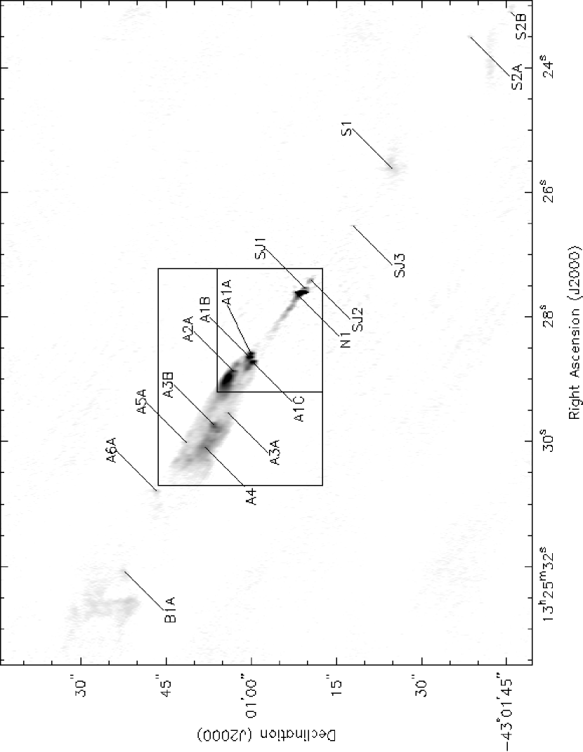
Figure 1: Radio knots in the jet and counterjet of Cen A. The map shown is the maximum-entropy 2002 A-array map, with $0\farcs 76\times 0\farcs 20$ resolution. Black is 10 mJy beam^-1. The transfer function is non-linear to allow low-surface-brightness structure to be seen. Knots are labeled according to a modified version of the notation of Clarke et al. (1992). The initial letter(s) and number denote the large-scale feature of which the knots form a part: the final letter (where present) distinguishes between sub-knots. N1 is the bright radio knot in the inner jet close to the nucleus seen by Clarke et al.. Boxes indicate regions of the jet that will be mapped in more detail in later Figures.

The high-dynamic-range images of the jet and counterjet (Fig. 1) give us two important pieces of information. Firstly, a number of compact faint radio knots are detected, including (for the first time) several clearly compact features in the large-scale counterjet region. (The inner counterjet knots denoted SJ1 and SJ2, and the large-scale features S1 and S2, had already been detected in the maps of Clarke, Burns & Norman [1992]). The new knots (A2A, A3A/B, A5A, B1A, SJ3, S2A, S2B) are all faint (with flux densities of at most a few mJy at 8.4 GHz) but are unambiguously detected in both VLA imaging epochs. As we shall see below (§4.2), several of the new faint radio knots are associated with comparatively bright X-ray emission.

Secondly, mapping the difference between the two epochs (or even simply blinking between the two maps) reveals that some, but not all, of the features in the jet have detectable proper motions along the jet. The most obvious motion is that of A1B, the middle knot in the bright base-knot complex, which has an apparent motion on the sky over the 11-year baseline of $0\farcs 101\pm 0\farcs 001$ in a position angle of 62° (defined in the sense north through east). The error quoted here is based on the errors returned by the aips Gaussian fitting task jmfit, fitting to both source and background, and so is likely to be optimistic, since it does not take into account systematic uncertainties due to, for example, the choice of fitting region: nevertheless, the proper motion is clearly detected. Further down the jet, the large-scale regions A2 and A3/4 appear to be moving coherently downstream. The apparent speed in these regions is hard to quantify, because there are few well-defined bright knots, but a measurement of the motion of the knot A3B, the brightest compact feature in this region, gives a proper motion of $0\farcs 06\pm 0\farcs 01$. By contrast, most of the compact features in the jet and counterjet (A1A, A1C, A2A, A3A, A5A, B1A, SJ1, SJ2, SJ3, S2A, S2B) had no detectable proper motion within the errors, although the accuracy of positions determined by fitting Gaussians to these features is low in the case of the fainter knots. In addition to the proper motions, the inner knot (A1A) has varied significantly (increasing in flux by 10%) over the epoch of observations, while the extended emission downstream of A1C appears to have become fainter.

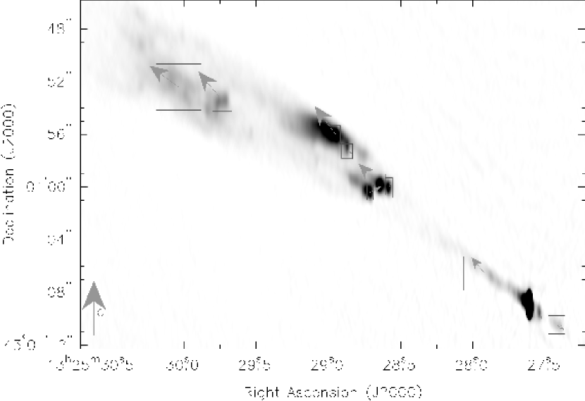
Figure 2: Motions in the jet between 2002 and 1991. The greyscale shows the 2002 A-configuration image, convolved to a resolution of $0\farcs 77\times 0\farcs 20$. Boxes indicate regions within which this image was compared with the 1991 image, convolved to the same resolution. Vectors show the best-fitting offsets between the two maps for each sub-image, exaggerated by a factor 20 for visibility. The vector in the bottom left-hand corner shows the offset that would be observed for a feature with an apparent speed of $c$. Note that only the four largest apparent motions are significantly detected; see the text for more details. This image shows the region of the jet denoted by the outer box in Fig. 1.

To confirm the reality of the apparent motions we used a version of the least-squares method discussed by Walker (1997), which involves shifting selected sub-regions of the jet so as to give the best match between the two epochs. The regions used in this method and the resulting best-fitting shifts are plotted in Fig. 2. The difficulties in applying this method to our data come from differences in background structure (due to slightly different short-baseline $uv$ coverage) coupled with real changes in knot structure, such as those seen in A1C. The best-fitting shift for the feature with the highest SNR, A1B, is in good agreement (within the errors) between the two methods: Walker’s method gives it a motion of $0\farcs 12\pm 0\farcs 03$ (errors are $1\sigma$, derived from the least-squared fits and based on estimates of the on-source noise). The motions determined for the compact features A1A and A2A are consistent with zero. A1C’s apparent backward motion, which is formally marginally significant, is a result of the changes in the knot structure discussed above. Further out, Walker’s method gives somewhat higher estimated speeds for the A3 region, $0\farcs 14\pm 0\farcs 03$. Although the motions in the inner jet and counterjet are not formally significant, they are plotted because of the suggestive directions of the best-fitting shift vector; it will be of interest to see whether these become significant in future monitoring.

The motion of knot A1B corresponds to an apparent speed on the sky of $0.51c$, based on the jmfit results, while the apparent speed in region A3 is between $0.3$ and $0.7c$ depending on the method used. We are therefore observing subluminal proper motions in the kpc-scale jet of Cen A, with apparent speeds higher than those observed in the parsec-scale jet and counterjet (Tingay et al., 1998). If the speeds are taken to represent the bulk speeds of the source, this would imply jet acceleration on scales between $\sim 1$ and 250 pc. It is more plausible that the motions of the parsec-scale knots (and possibly also of knot A1B) do not trace the bulk fluid flow in the jet, and in fact Tingay et al. argue that the variability of sub-components of the parsec-scale jet implies speeds $>0.45c$. A similar trend, in the sense that apparent speed increases with distance from the nucleus, has been observed in VLBI studies of some core-dominated objects (Homan et al., 2001).

If we assume that the component speeds in the kpc-scale jet do represent the bulk flow in the jet (and this seems inescapable in the outer parts of the jet, where the moving features are extended) then the combination of jet sidedness, assuming intrinsic jet symmetry, and observed motion allows us to set some constraints on the speed and angle to the line of sight of the jet. In general, the constraints from jet sidedness and variability on VLBI scales have suggested that Cen A is at a reasonably large angle to the line of sight ($\theta=50\arcdeg$ – 80°, Tingay et al. 1998): the small-scale jet-counterjet ratio $R$ is between 4 and 8 (Jones et al., 1996), and the model-dependent speed constraints ($\beta>0.45$) then require large angles to avoid obtaining $R>8$. The situation is interestingly different in the kpc-scale jet: $R>50$ at knot A1B (where the limit comes from taking the SJ3 component to be the brightest possible base knot counterpart), and even in the A3 region $R\sim 10$ (the faint extended region S1 is taken to be the counterpart of A3). These measurements, together with the observed motions, give the constraints shown in Fig. 3. Taken at face value, they require much smaller angles to the line of sight than has been estimated from the VLBI observations: in fact, the angles to the line of sight proposed by Tingay et al. are too large for any amount of beaming to be able to account for the jet-counterjet ratio in the A1 region (Fig. 3), let alone the relatively mild beaming implied by the observed sub-luminal proper motion. At least one of the assumptions involved in the various estimates of $\theta$ must be incorrect. Probably the jet and counterjet are not completely intrinsically symmetrical, since we know that the larger-scale inner lobes are asymmetrical both in their radio structure and their environments (Kraft et al., 2003): if this were true, some of the constraints would be relaxed, particularly those based on the limits on the sidedness near the compact A1 base knots, and it would be possible to obtain consistent values of $\theta$ from the sub-pc and 100-pc-scale data. Angles to the line of sight $\sim 50\arcdeg$ are also more plausible in interpretations of the large-scale radio and X-ray properties of the source (e.g., Kraft et al., 2003). This interpretation does leave unanswered the question of why the base region (A1) of the northern jet is intrinsically much brighter than that of its presumed southern counterpart.

The fact that the base knot A1A has apparently increased in flux density by around 10% can in principle give rise to some additional constraints on speeds. A Gaussian fit to this feature suggests a FWHM of about 0$\farcs$4, corresponding to 7.3 pc (23 light years). It is therefore impossible for the knot to have varied coherently on a timescale of a decade: it must contain some smaller-scale substructure, which is consistent with the relatively small amplitude of variation. Even so, the fact that it has changed so obviously suggests that significantly relativistic speeds must be involved, at least comparable to those estimated from proper motions further out. If this is true, the fact that the knot is stationary does not allow us to conclude that the bulk flow through the knot is slow.

4.1.2 Polarization structure

Our new observations give us good maps of the polarization structure in the inner jet, and these are shown in Fig. 4. They confirm the basic picture seen in earlier observations (Burns et al., 1983; Clarke et al., 1986) but have higher sensitivity and show more of the extended structure of the jet. We plot vectors perpendicular to the polarization $E$-vectors, which should be in the direction of the magnetic field in the emitting material if Faraday rotation is negligible, as we would expect it to be at this frequency from the rotation measure images of Clarke et al. (1992). The main point to note here is that the magnetic field direction appears to be almost entirely parallel to the jet over the whole region seen in these images (3 kpc along the jet), with the exception of a small region to the E and S of knot A2. There is no sign of the change to a transverse field direction along the center of the jet that is seen in some other FRI sources, and this appears to be the case on larger scales too (Clarke et al., 1992), although we do not detect polarization along the ridge-line of the large-scale jet. Accordingly, there is no evidence that we are seeing a region of the jet where a parallel component of the magnetic field at the edge might be thought to trace a slow-moving shear layer, as in some proposed models of jet deceleration and polarization structure (Laing, 1996). More recent versions of these models (e.g., Laing & Bridle, 2002a) do not predict a detectable transition to a transverse field direction in all cases. It is also interesting that the well-collimated inner part of the jet, before the flare point at knot A, appears to show a parallel field structure. This has been observed in some other sources (e.g., Owen et al., 1989; Hardcastle et al., 1996).

4.2 The radio/X-ray relation

4.2.1 Identification of radio and X-ray features

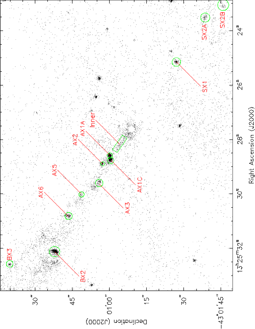
Figure 5: The X-ray emission from the Cen A and counterjet. Extraction regions for some of the X-ray features are labeled. The greyscale shows the raw counts in the energy band 0.4–2.5 keV, with $0\farcs 123$ pixels. This image shows the same region of the jet as Fig. 1.

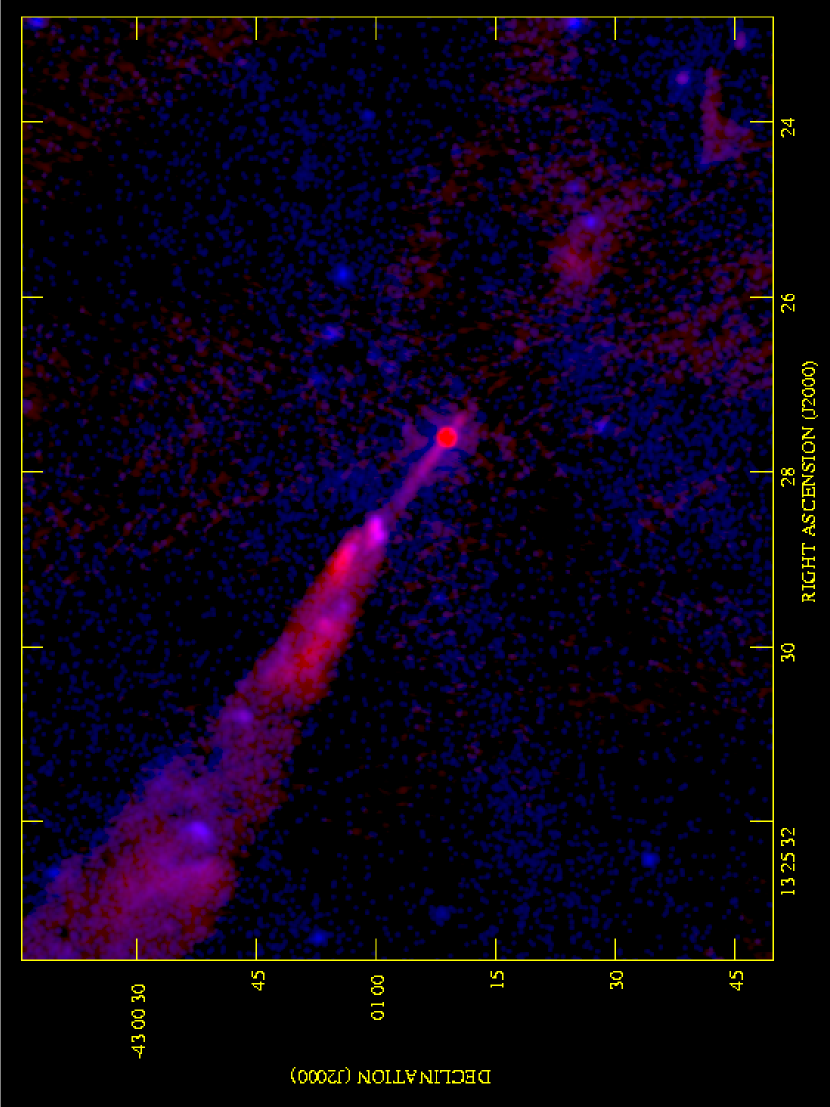
Figure 6: The X-ray and radio structure of the Cen A jet. The X-ray image, made from events with energies between 0.4 and 2.5 keV, is in blue and the radio image, made with imagr from the combined-epoch A- and B-configuration data, is in red. The X-ray data have been smoothed with a Gaussian and the restoring beam of the radio map has been chosen so that both radio and X-ray data have a resolution (FWHM) around $0\farcs 85$. The transfer function is non-linear to allow low-surface-brightness structure to be seen. This image shows the same region of the jet as Fig. 1.

The new X-ray and radio data allow a more detailed comparison to be made between the two wavebands than was previously possible. The most striking new results are the good detection (in X-rays and radio) of the inner, well-collimated part of the jet, and the association of several previously known X-ray knots with faint compact radio features. Fig. 5 shows the quality of the new X-ray data, while Fig. 6 shows a comparison of the radio and X-ray structures. The unprocessed resolutions of the data are somewhat different: the Chandra PSF close to the core can be fitted as a circular Gaussian with FWHM $\sim 0\farcs 65$, while the radio data have an elongated beam, as discussed above. To simplify comparison in Fig. 6 we have smoothed the X-ray emission with a $0\farcs 5$ Gaussian kernel and used a circular restoring beam in the radio mapping (after appropriate weighting of the $uv$ plane) so that both images have a resolution of $\sim 0\farcs 85$ (the FWHM of a circular Gaussian) close to the core. The effective resolution of the Chandra data is somewhat lower ($\sim 0\farcs 95$) at the furthest distances from the core shown on this Figure, but we do not regard this as a significant problem.

It is clear from these images that some of the previously known X-ray knots in the jet (AX2, AX3, AX5, AX6, BX2 in the notation of K02, as used in Fig. 5) are associated with the newly discovered weak radio knots: AX2 with A2A, AX3 with A3A, AX5 (or part of it) with A5A, AX6 with A6A and BX2 with B1A. In addition, the two X-ray knots SX2A and SX2B are coincident with the counterjet radio features S2A and S2B. In the jet, extended X-ray emission is associated with most, but not all, of the radio emission region: for example, there is no strong X-ray emission associated with the bright extended region A2 (as opposed to the weak compact knot A2A). In several places there is brighter radio emission downstream of a faint radio knot associated with an X-ray feature: this is true of the radio features A2, A3 and B.

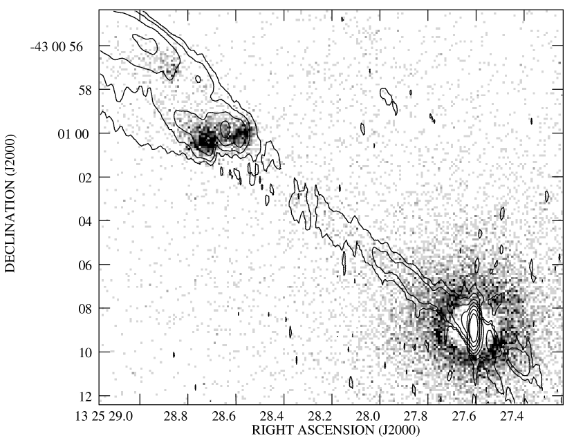
Figure 7: The inner part of the Cen A X-ray and radio jet. The contour plot shows the A-array 2002 maximum-entropy map with resolution $0\farcs 76\times 0\farcs 20$, with contours at $200\times(1,4,16,64\dots)$ $\mu$Jy beam^-1, while the greyscale shows the 0.5-7.0 keV X-ray data binned in 0$\farcs$0984 pixels (effective resolution $\sim 0\farcs 65$). Black is 6 counts per pixel; the central parts of the X-ray nucleus are strongly affected by pileup and so no valid counts are seen. This image shows the region of the jet denoted by the inner box in Fig. 1.

The results show that the radio to X-ray flux density ratio is strongly variable as a function of position in the jet. Some radio regions have comparatively strong radio emission and weak X-ray emission (for example region A4) while others, of which the radio knot B1A is probably the clearest example, have strong X-ray emission and weak radio emission. There are some X-ray sources in or near the jet which have no detectable radio counterparts. The X-ray feature BX3 is an example of this, although it is possible that it is unrelated to the jet (as suggested by its point-like X-ray appearance compared to other jet sources: if it is unrelated to the jet, it is most probably a LMXB associated with NGC 5128). Equally, there are comparatively bright radio features with no X-ray detections. This is true of the counterjet features SJ2 and SJ3 (Fig. 6). As Fig. 7 shows, there are also strong differences between the X-ray properties of the knots in the bright A1 region (in this figure we retain the full resolution of both datasets for clarity). The knot A1B, the brightest of the three in the radio, has by far the faintest X-ray emission. In the following subsection, we investigate the radio and X-ray spectra of these regions quantitatively.

4.2.2 X-ray spectroscopy and flux densities for compact features

We extracted spectra and flux densities for all the compact X-ray features associated with radio knots, together with the corresponding radio flux densities. Fig. 5 shows some of the extraction regions, and the results are tabulated in Table 2; total counts in the knots vary between $\sim 1000$ for the brightest features and $\sim 100$ for the faintest. In each case we fitted a power-law model absorbed with a free, zero-redshift absorbing column (which in general includes both the Galactic column density, $\sim 7\times 10^{20}$ cm^-2, and the much larger column from the dust lane of Cen A). We included the effects of the reduced quantum efficiency of the detector at the epoch of observations by using the acisabs model to correct the response files. The X-ray flux densities quoted are the unabsorbed values. We determined background using nearby, off-jet background regions. All the fits were good. The corresponding radio flux densities are those of the compact features, measured where possible by fitting a Gaussian and background level to the radio images. We also tabulate, in parentheses, the total radio flux densities (including flux from any extended background emission seen in the A-array map) in the regions corresponding to the X-ray extraction regions, which provides an upper limit on the radio emission from the X-ray features. In some cases this total flux density is a very conservative limit, as it includes part of another radio feature: this is true of knots A1A and A1C (contaminated by A1B) and A2A (contaminated by extended emission from the A2 region). We find that the radio to X-ray flux ratios of the different knots vary by more than an order of magnitude, and the best-fitting X-ray spectral indices for radio-associated features range from 0.3 to 1.4. Fig. 8 gives a graphical representation of the differences in the properties of the knots.

The column densities inferred from the spectral fits, and tabulated in Table 2, are consistent with a single value of the absorbing column, $\sim 6\times 10^{21}$ cm^-2, in the inner regions of the jet (AX1–6), as reported by K02. In knot BX2 and in the counterjet features, the absorbing column density is lower, and is generally consistent with the Galactic value. This is qualitatively as we would expect from sensitive imaging of the dust features in Cen A (e.g., Schreier et al., 1996); the entire inner part of the jet lies in the dust lane.

Table 2: X-ray and radio features of the jet

X-ray name	Radio name	Radio flux	X-ray flux	$S_{\rm X}/S_{\rm R}$	$\alpha_{\rm RX}$	$\alpha_{\rm X}$	$N_{\rm H}$ ($\times$
		density (mJy)	density (nJy)	($\times 10^{-6}$)			$10^{22}$ cm-2)
AX1A	A1A	28.2 (74)	$41^{+8}_{-6}$	1.48 (0.56)	0.78	$1.30_{-0.26}^{+0.28}$	$0.61_{-0.13}^{+0.14}$
AX1B	A1B	51.2 (69)	$24^{+18}_{-11}$	0.47 (0.35)	0.85	$1.9_{-0.8}^{+1.0}$	$1.04_{-0.47}^{+0.60}$
AX1C	A1C	40.7 (113)	$47^{+6}_{-5}$	1.20 (0.43)	0.80	$1.05_{-0.18}^{+0.19}$	$0.47_{-0.08}^{+0.09}$
AX2	A2A	11 (50)	$3.2_{-0.5}^{+2.9}$	0.31 (0.07)	0.88	$0.1_{-0.3}^{+0.8}$	$0.004_{-0.004}^{+0.6}$
AX3A	A3A	2 (25)	$13^{+7}_{-4}$	6.5 (0.52)	0.70	$1.4_{-0.3}^{+0.7}$	$0.56^{+0.36}_{-0.29}$
AX6	A6A	3.0 (5.6)	$10^{+3}_{-2}$	3.3 (1.8)	0.73	$0.36_{-0.41}^{+0.42}$	$0.43_{-0.23}^{+0.29}$
BX2	B1A	2.5 (7.8)	$23_{-2}^{+2}$	9.7 (3.1)	0.68	$0.56_{-0.14}^{+0.15}$	$0.06_{-0.04}^{+0.04}$
BX3	–	$<1$	$2.3^{+0.7}_{-0.2}$	$>1.9$	$<0.76$	$0.2_{-0.5}^{+0.7}$	$<0.20$
SX1	–	$<0.5$	$9^{+3}_{-2}$	$>18$	$<0.64$	$0.44_{-0.40}^{+0.42}$	$0.22_{-0.20}^{+0.22}$
SX2A	S2A	2 (2)	$3.2_{-0.5}^{+1.4}$	1.7 (1.7)	0.78	$0.45_{-0.40}^{+0.65}$	$0.04_{-0.04}^{+0.22}$
SX2B	S2B	2 (2)	$2.1_{-0.3}^{+1.0}$	0.9 (0.9)	0.80	$0.5^{+1.2}_{-0.7}$	$<0.33$
Inner	Inner	28	$38_{-24}^{+98}$	1.43	0.79	$2.2_{-1.7}^{+2.5}$	$1.1_{-0.8}^{+1.2}$
Extended	Extended	1300	$86_{-5}^{+6}$	0.07	0.96	$1.00_{-0.15}^{+0.16}$	$0.11_{-0.03}^{+0.03}$

Note. — Errors quoted for $\alpha_{\rm X}$ and $N_{\rm H}$ are the $1\sigma$ error for two interesting parameters ($\Delta\chi^{2}=2.3$), since these two quantities are strongly correlated in the fits. For consistency, the limits quoted on the column density in the two cases where the best-fitting value is formally zero are also $1\sigma$ limits. The errors on the unabsorbed 1-keV flux densities are $1\sigma$ for one interesting parameter ($\Delta\chi^{2}=1.0$).

4.2.3 Sizes of X-ray features

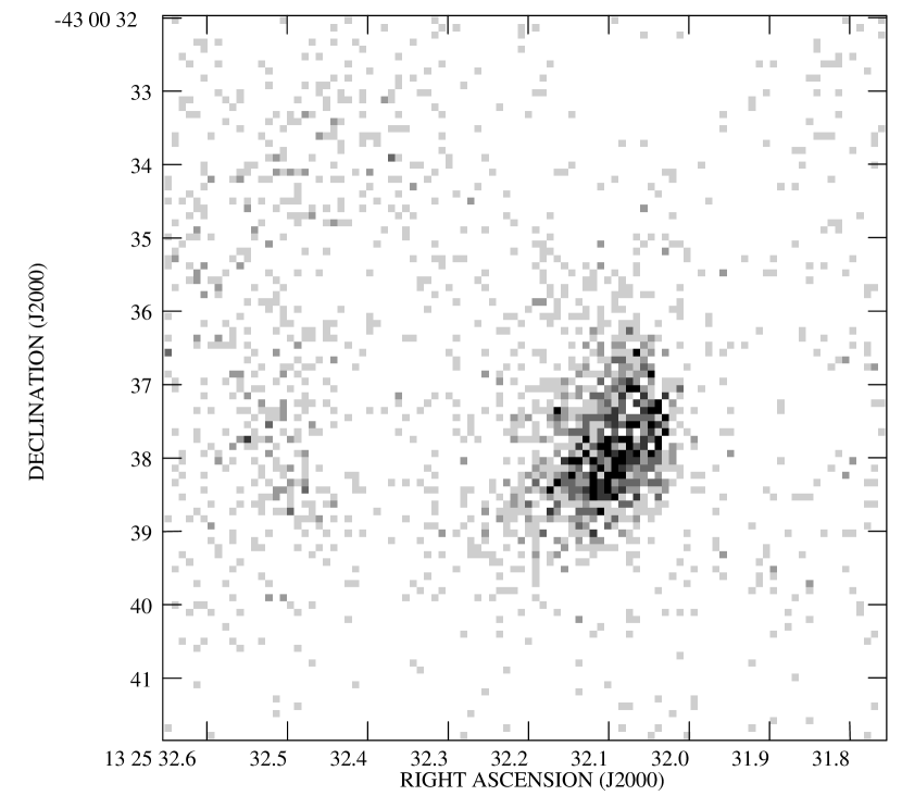
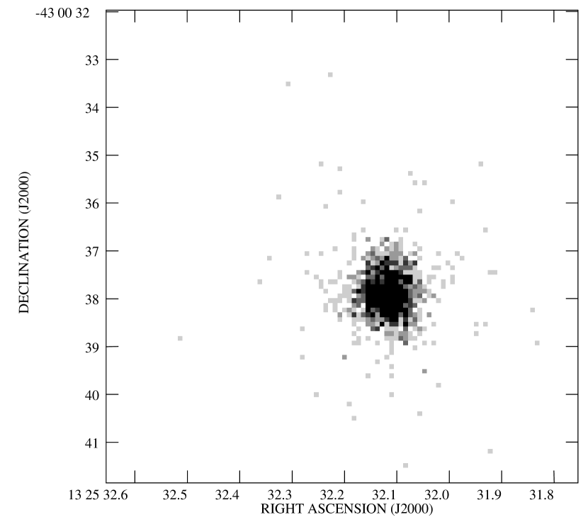
Figure 9: The detailed structure of knot BX2 (left) and a simulated point-spread function normalized to have the same total counts within 2″ (right). BX2 is clearly extended on scales of approximately 1″. One pixel is $0\farcs 0984$ and black is 5 counts per pixel. See the text for details of the simulations used.

We noted in K02 that several of the X-ray knots in the jet appeared to be significantly extended. Some of these (the most obvious example being AX1: Fig. 7) are now seen to have sub-structure on scales smaller than the resolution of the data that was then available to us. Knot BX2, by contrast, appears to be genuinely resolved in our new data. Fig. 9 shows a comparison between the observations and a simulation, using the web-based ray-tracing tool ChaRT, of the Chandra point-spread function at this position for the observed energy distribution of BX2. Visual inspection and radial profiling both show that BX2 is resolved transversely to the jet direction, on scales of 1″. This extension is also present in the radio data, though the elongated radio beam makes it less obvious. We have searched for X-ray extension in the other isolated, compact radio-related knots such as AX6 and found little significant evidence that it is present, which implies sizes in the X-ray $\lesssim 0\farcs 5$ ($\lesssim 10$ pc); these are again consistent with the radio observations. The complex structure of the AX1 region means that a full deconvolution, which we have not carried out, would be required to derive good constraints on structure in the X-ray sub-knots, but we believe that both bright X-ray knots are probably marginally extended on scales $\sim 0\farcs 5$.

4.2.4 The extended X-ray and radio emission

We extracted two spectra for extended regions of the jet. These were the faint inner jet between the nucleus and knot A1, and the extended emission in the jet between knot A2 and the knot B region, excluding all compact X-ray features. In both cases we used an off-source background region of the same size at the same radial distance from the nucleus. The radio emission was measured from the corresponding regions of the multi-epoch, A+B-configuration images without background subtraction. The results are tabulated in Table 2. Note that the X-ray to radio flux ratio for the extended jet is much lower than for any individual jet knot.

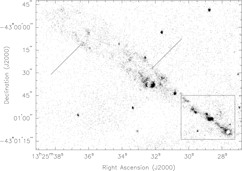
Figure 10: The X-ray structure of the large-scale Cen A jet. The greyscale shows the raw counts in the 0.4–2.5 keV band; the pixels are $0\farcs 492$ on a side and black is 12 counts per pixel. The lines indicate two regions where the X-ray jet appears significantly edge-brightened (see the text). The box, shown for orientation purposes only, shows the region denoted by the outer box in Fig. 1.

The X-ray emission on scales larger than that of the inner jet is shown in Fig. 10. Generally the extended X-rays are reasonably well matched to the radio emission on these scales; in particular, diffuse X-ray emission clearly extends to the edge of the radio jet. There are some faint compact X-ray features, identified by K02, which have no apparent compact radio counterparts, though we cannot rule out the possibility that their radio counterparts are simply too faint to be convincingly detected. To the north and downstream of the bright X-ray knot BX2 the extended X-rays appear to be associated with the edge of the jet, and to be absent in the jet center. A similar region of edge-brightening is seen further down the jet. These regions are marked with lines on Fig. 10; neither has a counterpart in the large-scale radio emission. Their detection raises the possibility that the edges of the jet, which are the locations where jet mass entrainment takes place in the standard FRI jet model (e.g., Laing & Bridle, 2002a) are privileged sites for the particle acceleration required to generate the X-ray emission.

5 Discussion

5.1 Radio supernovae?

Although the X-ray knots with detected radio counterparts cannot be X-ray binaries in Cen A, since such objects have at most extremely weak radio counterparts, it is not out of the question that they could be jet-associated radio supernovae (SN) or supernova remnants (SNR). Capetti (2002) has suggested that in some cases type Ia supernovae may be triggered by jets. X-ray emission of luminosity comparable to that of the X-ray knots in Cen A (K02) is most likely to be produced by type II supernovae in dense environments rather than by SNIa, but there is evidence (Graham & Fassett, 2002) that the jet is inducing star formation in the host galaxy, so that this is not impossible. The radio luminosities of the weaker knots, with fluxes of a few mJy, are comparable to those of known SNR in M82 (Muxlow et al., 1994), which lies at a very similar distance, and at least some of the M82 sources have tentative X-ray associations of similar luminosity to the Cen A knots Matsumoto et al. (2001), although a full analysis of the M82 Chandra data has not yet been published. The main fact that convinces us that the Cen A knots are not related to supernovae is their good power-law spectra. The emission from a young SNR in a dense environment is expected to be thermal and to have a comparatively low temperature, $\lesssim 1$ keV (e.g., Fabian & Terlevich, 1996) while the only thermal models that can be fitted to flat-spectrum sources like BX2 require high temperatures ($>6$ keV at the 90% confidence level) and very low metal abundance. We therefore assume in what follows that the radio and X-ray knots reflect structures in the fluid flow in the jet.

5.2 Knot properties

We can rule out the possibility that the X-ray bright, radio-faint knots are simply compressions in the synchrotron-emitting fluid that makes up the extended jet. As an example, we consider the case of knot BX2, which has a well-constrained, flat $\alpha_{\rm RX}$ and $\alpha_{\rm X}$. The extended jet has a steep $\alpha_{\rm RX}$ and $\alpha_{\rm X}$, and so, if we model its spectrum as a simple broken power law in frequency, with a low-frequency (radio) spectral index similar to the $\alpha_{\rm RX}$ of BX2, the break to a steeper spectral index must occur at comparatively low frequencies, $\nu_{\rm b}\sim 10^{12}$ Hz. For adiabatic compression of this material to produce the spectrum seen in knot BX2, where the break frequency would be above the soft X-ray band ($\nu_{\rm b}\gtrsim 5\times 10^{17}$ Hz), we require 1-dimensional compression factors $\cal R$ of about 30, since $\nu_{\rm b}\propto{\cal R}^{-4}$ for a tangled field geometry (Leahy, 1991). But such high compression factors would increase the radio volume emissivity of the knot over that of the parent material by a factor $\sim 10^{11}$ ($j_{\nu}\propto{\cal R}^{-(5+4\alpha)}$), whereas the ratio of the volume emissivities of the knot and extended jet (assuming spherical symmetry for the one and a truncated-cone geometry with uniform filling factor for the other) is $\sim 2$. BX2 is an extreme case, but similar arguments apply to the other compact jet features.

Instead, it must be the case that the knots are privileged sites for the in situ particle acceleration that is required throughout the jet. For the the base knots (AX1A, AX1C) this is not particularly surprising; these are presumably related to the transition between the faint, well-collimated, efficient inner jet and the much brighter extended jet (Fig. 7). They can be modeled as standing shocks at the base of the jet, and we cannot even rule out the possibility that their radio-to-X-ray spectra are described by a standard continuous injection model (e.g., Leahy, 1991), as used to describe the hotspots in FRII radio sources, in which the spectral index steepens from $\sim 0.5$ to $\sim 1.0$ at some frequency.

What does this imply for the weaker knots — AX2, AX3A, AX6, BX2 and the counterjet features? One clue is provided by the fact that none of the radio counterparts of these features appears to be moving with the jet flow, although for some of them (AX2, AX3A, AX6) there is nearby and downstream apparently moving structure. This strongly suggests that these features are also standing shocks in the jets, which is consistent with the observation that at least one of them is extended perpendicular to the jet direction (§4.2.3). It is very hard to imagine a model purely related to the fluid flow in the jet that would give rise to this kind of localized stationary shock after the jet flare point at knot A1. Instead, the shocks must be related to some feature of the jet’s environment that is fixed or slowly-moving in the galaxy frame, a point we return to below (§5.3).

By contrast, the features that are clearly moving in the radio images (A1B, A2, A3/A4) have comparatively little X-ray emission; A2 and A4 in particular appear to have X-ray to radio ratios less than the values typical for the extended jet as a whole. For the speeds inferred from the proper motion and sidedness constraints (Fig. 3) the Doppler factor is $>1$ in these regions, so beaming, for a fixed spectral shape, would tend to increase the observed X-ray to radio flux density ratio (since the spectral index of the X-ray-emitting material is steeper than the radio spectral index, so that the $K$-correction is greater). So it is likely that the high-energy particle acceleration in these regions is less efficient than in the jet as a whole. This would again be consistent with a picture in which the distributed particle acceleration process is more efficient in the slower-moving edges of the jet than in the faster-moving regions which we would expect to be closer to the jet center.

The detection of some large-scale counterjet X-ray features with associated radio knots confirms that there is continuing energy transport, and thus presumably collimated outflow, on scales of $50^{\prime\prime}$ or 850 pc, projected, from the core on the counterjet side of Cen A. It is still not clear whether the 6 or so X-ray features without radio counterparts that lie in the inferred counterjet region (Fig. 6) are all related to the counterjet. The properties of the brightest of these, SX1 (Table 2), are extreme compared to those of the jet knots, but we cannot rule out a flat-spectrum power law ($\alpha\sim 0.5$) extending from the radio to the X-ray, which would give rise to a radio flux density around 50 $\mu$Jy; our radio images are still not quite sensitive enough to detect this.

5.3 Standing shocks

If the radio-weak, X-ray bright, stationary or slow-moving knots in the post-A1 region are indeed standing shocks in the jet, then we would expect them to be related to some feature of the jet environment approximately fixed in the frame of the host galaxy. Here we concentrate on models in which the jet is interacting with discrete, compact objects (Blandford & Königl, 1979). We can obtain a constraint on the mass of these objects from the fact that they are not observed to move. The minimum energy density $\epsilon$ in the jet is of order a few $\times 10^{-11}$ J m^-3. If we assume that the bulk flow speed $v_{j}\sim 0.5c$ (i.e. only mildly relativistic, with Lorentz factor $\sim 1$), then a limit on the mass $M$ of an object not moving visibly with the flow is given by

$$M\gtrsim\pi R^{2}\epsilon\left({v_{j}\over c}\right){t\over v_{l}}$$

where $v_{l}$ is the minimum speed of proper motions that we could observe (say $0.1c$), $R$ is the radius of the object, and $t$ is the length of time that the object has been experiencing the thrust from the jet; we assume that the kinetic energy density of the jet dominates its mass-energy density, as is the case for a plasma consisting only of relativistic electrons. Considering the minimum energy in the inner lobes ($E\sim 2\times 10^{48}$ J) and requiring that this should have been supplied by the jet, $E\approx\epsilon A_{X}v_{j}t$ where $A_{X}$ is the cross-sectional area of the jet, we obtain $t$ of the order of a few $\times 10^{6}$ years, which we can treat as a limit on the timescale that the jet has been currently active (clearly the total energy in the middle and outer lobes of Cen A is much larger, but these may well be the results of earlier epochs of AGN activity.) Taking $R$ to be comparable to the sizes of the smaller radio knots, $\sim 10$ pc, and using a jet radius of 60 pc, we obtain values of $M$ for the obstacle of the order of a few solar masses (or more). $M$ can be less than this if $R$ or $t$ are less than our estimates. Given the velocity dispersion in NGC 5128 (Israel, 1998), the time for an individual star to cross the jet would be of order a few $\times 10^{5}$ years, which would relax the limit on $M$ somewhat. On the other hand, there is no particular reason to believe that the energy density in the jet is the minimum energy, and some evidence that it is greater for FRI jets (e.g., Laing & Bridle, 2002b) which would increase the required mass.

We expect that there will be $\sim 10^{9}$ stars in the inner kpc of the galaxy (the region including the compact knots) and so the jet would be expected to include a few $\times 10^{6}$ stars at any given time: even if stars are ablated rapidly by the jet, new stars would enter from the edges on short timescales. Clearly the particle acceleration regions cannot be associated with individual normal stars, although it is possible that ‘shocklets’ around each star contribute to the required diffuse high-energy particle acceleration which occurs throughout the jet.

The objects responsible for the discrete radio and X-ray features (AX2, AX3A, AX6, BX2 and the counterjet features) must be considerably rarer than normal stars. Possibilities include high-mass-loss stars (e.g. Wolf-Rayet stars) and entrained gas clouds. The size of the interaction region $r_{w}$ for a high-mass-loss star is given by ram-pressure balance between the stellar wind with speed $v_{w}$ and the jet:

$$r_{w}=\left({\dot{M}v_{w}c^{2}\over 4\pi\epsilon v_{j}}\right)^{1\over 2}$$

and so, for a Wolf-Rayet with a mass-loss rate $\dot{M}$ of $10^{-4}M_{\odot}$ yr^-1 and $v_{w}\sim 2000$ km s^-1 we can readily obtain scale sizes of the order of 10 pc if the jet is near its minimum energy density. These are rather extreme properties even for a Wolf-Rayet, however (e.g., Nugis & Lamers, 2000), and would require what is a rather large (though not impossibly large) number of Wolf-Rayets per normal star, given the stellar densities estimated above; the Wolf-Rayet fraction is known to depend strongly on the star formation rate.

On the other hand, various types of gaseous material are present in the inner part of the galaxy. Hot gas is known to be present from its thermal X-ray emission, but its central density is only $3.7\times 10^{-2}$ cm^-3 (Kraft et al., 2003) which means that a 10-pc-diameter cloud would be a factor of a few below our derived lower mass limit. Molecular material is known to be present in the inner part of Cen A, particularly the dust lane (e.g., Wild & Eckart, 2000): for a density of $\sim 300$ cm^-3, a 10-pc-diameter molecular cloud would have $8\times 10^{3}\ M_{\odot}$, which is certainly not excessive given the estimated total molecular hydrogen mass of $4\times 10^{8}\ M_{\odot}$ (Israel, 1998), and more than satisfies the constraints on mass derived above. $10^{4}$-K line-emitting material, which is known to be associated with the inner jet (Brodie, Königl & Bowyer, 1983) as well as being present on larger scales (Morganti et al., 1991) would have similar or somewhat lower densities to molecular material, and would be equally suitable as obstacles if the clump size was great enough; alternatively, the line emission seen by Brodie et al. 1983 could be the result of stripping and shock-excitation of colder material. In any case, we consider interaction with clouds of cold or warm gas to be more likely than interaction with high mass-loss stars as the explanation for the stationary radio and X-ray knots in Cen A.

Finally, it should be borne in mind that Cen A’s jet is probably an order of magnitude lower in kinetic luminosity than the jets in well-known 3C FRI sources with X-ray jets like 3C 31 and 3C 66B. This means that the stellar-wind interaction model, at least, is probably not viable as an explanation for any X-ray/radio features in those jets. Interaction with external gas clouds is still a possibility, but Cen A’s host is probably richer in molecular material than a typical FRI host elliptical.

5.4 The nature of ‘offsets’

The data for Cen A emphasize the importance of high spatial resolution in discussing apparent offsets between the radio and X-ray peaks in FRI jets. The strong variation in X-ray to radio flux ratio as a function of position that we observe in Cen A could give rise to apparent offsets between the peaks of unresolved or poorly resolved knots in more distant sources. For example, if Cen A were placed at the approximate distance of a well-studied nearby FRI like 3C 66B ($z=0.0215$), the resolution of Chandra and the VLA would correspond to tens of arcsec on Fig. 6. The knot B region would then be essentially unresolved, and would present a classical example of an offset between the radio and X-ray peaks, entirely because of the very different $\alpha_{\rm RX}$ values of BX2 and the remaining downstream regions of knot B. In order to make an adequate model of the physics underlying the ‘offset’ behavior, it is necessary to have radio and X-ray data with spatial resolution sufficient to sample the jet structure on the physical scales of interest. Unfortunately, Cen A is at present the only source for which that is true.

It is still of interest to ask why the observed ‘offsets’ are always in the sense that the X-ray peak lies closer to the nucleus. We suggested (Hardcastle et al., 2001) that the offsets in knot B of 3C 66B could be modeled in terms of a particle-accelerating shock together with downstream advection of radio-emitting particles, while the X-ray-emitting electrons would be rapidly quenched by synchrotron losses and/or expansion (a model subsequently discussed in more detail by Bai & Lee [2003]). Of the features in Cen A, region A2 comes closest to this simple picture (Fig. 11). Almost all the X-ray emission comes from a region coincident with a very faint compact radio knot (A2A); downstream there is bright radio emission with little or no corresponding X-ray. The X-ray profile is certainly what we would expect from a model with particle acceleration and downstream advection. But this model does not simply explain the clear separation ($1\farcs 3$, or 20 pc) between the faint knot A2A, coincident with the X-ray peak, and the peak of the radio emission. If the downstream advection were uniform, then, for a static region of particle acceleration, we would expect the radio profile to be brightest at the same place as the X-ray, and then to fade more slowly as a function of downstream distance. This model would explain the observed offsets in other, more distant sources, but it is not consistent with what we actually see in Cen A. If we require all the radio-emitting particles in the A2 region to have been accelerated at A2A, then we need, at least, non-uniform downstream advection to cause them to ‘pile up’ at the A2 peak.

There are two other areas in the inner jet where bright radio emission is seen downstream of a faint radio/bright X-ray knot, in the regions of knots A3/4 and B. These depart even more clearly from the expected behavior in the simple downstream advection model. Fig. 11 shows that the weak radio knot A3A, coincident with the brightest X-ray emission, leads the radio peak (A3B) by about 3″ (50 pc). However, in this case, there is X-ray emission from the radio peak too. In knot B, the X-ray peak, coincident with the radio knot B1A, is separated by around 8″ (140 pc) from the peak of the downstream diffuse emission, which again shows some weak X-ray emission.

We cannot rule out the possibility that the apparent association between weak upstream radio knots with bright X-ray emission and bright downstream diffuse radio features with faint X-ray emission is coincidental. There are only three clear cases, and other knots (such as A6 and the counterjet features) do not have bright downstream emission. However, if it is not coincidental, then it is certainly giving us information about the properties of the fluid flow. For example, if the compact knots are standing shocks in the flow, caused by interaction with static obstacles (§5.3) then it is conceivable that the bright downstream radio emission is due to compression and/or turbulent particle acceleration as the post-obstacle flow re-joins the main jet. In this case the downstream distance $d$ and the size of the obstacle $R$ would give us an estimate of the internal Mach number of the jet, ${\cal M}\approx d/R$. The knot-to-peak distances for A2A and A3A are respectively about 20 and 50 pc, which would lead to estimates of ${\cal M}$ of approximately 2 and 5 respectively for our adopted obstacle size of $\sim 10$ pc. (As the peak downstream distance for knot B is not well defined, we do not include it here.) These Mach numbers are at least in the expected region for the base of an FRI jet, being mildly supersonic, and (given our proper motion results) would imply relativistic internal sound speeds in these regions of the jet.

Finally, we note that offsets between the peak positions of radio and X-ray knots have been seen in the other extragalactic jet where comparatively high spatial resolution is available, M87’s (Wilson & Yang, 2002), where 1″= 78 pc. The peak-to-peak distances in the M87 knots that show offsets are also tens of parsecs, consistent with what we find above for the knots in Cen A, although the M87 jet is clearly rather physically different from Cen A’s (being somewhat narrower and much smoother) in the regions where the offset is observed. Based on our results above, we would predict that X-ray knots D and F in M87 are actually coincident with faint, as yet unseen features in the radio jet. If this is the case, the good optical information available for M87’s jet should place interesting constraints on the knot spectra.

5.5 The inner jet

The detection of the well-collimated inner jet in both radio and X-rays is of interest because, in the standard model of FRI radio sources, this represents the efficient, supersonic flow that transports energy up to the point where the jet disrupts and becomes trans-sonic and turbulent (which would be at knot A in Cen A). These jets are efficient in the sense that their radio luminosity per unit length is much less than is observed after the flare point. However, the detection of X-ray emission from these regions (in addition to Cen A, the inner jets of M87 [Wilson & Yang 2002] and 3C 66B [Hardcastle et al. 2001] have been detected in the X-ray) is of interest because, if it is synchrotron in origin, it shows that this region of the jet is still capable of in situ particle acceleration. In M87 and 3C 66B the inner jet has a considerably higher X-ray to radio ratio than the regions further from the nucleus. In Cen A the situation is complicated by the poorly constrained absorbing column in this region, which means that the unabsorbed flux density of the jet is uncertain (Table 2) but it is still clearly the case that the X-ray to radio ratio is higher than that in the extended jet as a whole, though probably not higher than those of some of the compact knots. (Here we assume, since the spatial resolution is insufficient to allow us to do anything else, that the X-ray and radio emission from the inner jet come from the same regions.) Unlike the M87 and 3C 66B inner jets, Cen A’s shows little evidence in radio or X-ray for knotty sub-structure which might be associated with oblique internal shocks giving rise to particle acceleration, while other possible particle acceleration mechanisms (such as second-order Fermi acceleration or turbulent magnetic field line reconnection) would be expected to be more efficient in the trans-sonic large-scale jet. Doppler boosting may be important here, particularly given the steep best-fitting X-ray spectral index. The observed X-ray to radio ratio goes as ${\cal D}^{(\alpha_{\rm X}-\alpha_{\rm R})}$ and so, to bring the ratio in the inner jet in line with that in the extended jet (assuming little Doppler boosting in the latter), we need an inner jet Doppler factor $\sim 6$ (with a large uncertainty due to the uncertainty in the inner jet flux density and spectral index). Doppler factors of this order would require $\theta\lesssim 10\arcdeg$, which is more or less possible given the constraints of Fig. 3, though, as we suggest above, such small angles to the line of sight are unlikely for other reasons. Nevertheless, we cannot rule out the possibility that rapid bulk motion in Cen A’s inner jet is responsible for its high X-ray to radio flux ratio. If this were the case, the radio emission from the jet as we observe it would be boosted by a large factor, so that in reality it would be still more efficient in transporting energy.

6 Summary and conclusions

1. Our high dynamic range radio images of Cen A reveal subluminal apparent motions ($v\sim 0.5c$) in the hundred-parsec scale jet. Some extended regions of the jet appear to be moving coherently downstream, which suggests that the apparent speeds may be close to the bulk jet speed. If this is the case, and if the jet and counterjet are symmetrical, Cen A must make a comparatively small angle to the line of sight ($\theta\sim 15\arcdeg$), which contrasts with the larger angles inferred from the parsec-scale properties of the source.

2. We have discovered faint radio counterparts to a number of the previously unidentified X-ray knots in the inner parts of the jet, demonstrating that the X-ray features are jet-related.

3. We also detect radio counterparts to some X-ray features on the counterjet side, suggesting that there is collimated flow on kpc scales in the counterjet region.

4. If the X-rays from the compact knots are due to synchrotron emission, then the radio to X-ray and X-ray spectra allow us to rule out a model in which the knots are simply compressions in the fluid flow: instead, they must be privileged sites for high-energy particle acceleration.

5. Almost all the strongly X-ray emitting knots appear to have radio counterparts that are static within the limits of our observations, suggesting that they trace stationary shocks in the jet flow. Plausibly they are the result of an interaction between the jet fluid and an internal obstacle such as a high-mass-loss star or molecular cloud. By contrast, the radio jet features that are apparently moving show weak or absent X-ray emission, although there is still diffuse X-ray emission throughout the jet that is not identified with discrete radio features.

6. Several of the radio-faint, X-ray-bright knots are associated with downstream bright radio emission, and we suggest that it is this behavior, seen at lower resolution, which gives rise to the observed offsets between the radio and X-ray peaks in some more distant FRI jets. The simplest possible model with particle acceleration and downstream advection does not explain the details of these observations.

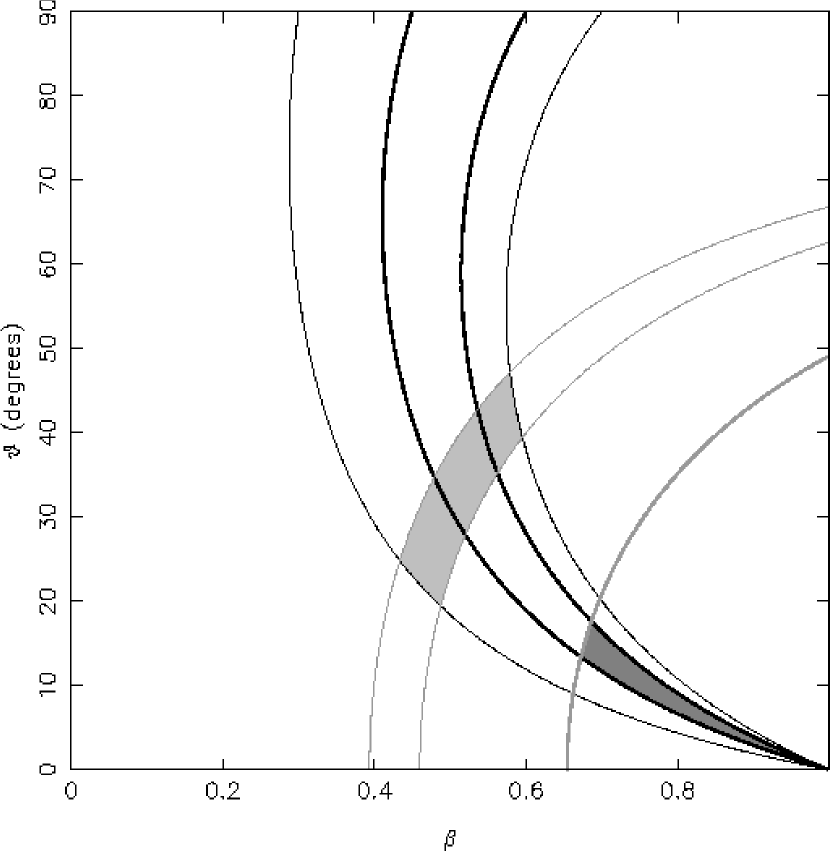
Figure 3: Constraints on the permitted values of the bulk speed and angle to the line of sight from the jet-counterjet ratio and apparent motions in the A1B and A3 regions of the Cen A jet. Thick lines represent constraints on A1B, thin lines show constraints on A3. The gray lines show the constraints from sidedness, the black lines show the constraints due to apparent motions), and the intersection between the regions (shaded in light gray) shows the permitted regions of parameter space for the two components. The spacing between the lines indicates an approximate estimate of the uncertainties on sidednesses and proper motion speeds. Sidedness ratio calculations are carried out with the form of the sidedness relation appropriate to a continuous jet. Note that only small angles to the line of sight ($\theta\sim 20\arcdeg$) are consistent with all the observations.

Figure 4: Polarization structure in the jet of Cen A. Top: the inner jet, image made from the 2002 A-array data with $0\farcs 76\times 0\farcs 20$ resolution (this image shows the region of the jet denoted by the outer box in Fig. 1). Bottom: the larger-scale jet, image made from the 2002 B-array data with $3\farcs 20\times 0\farcs 73$ resolution. Contours are at $200\times(1,4,16,64,\dots)$ $\mu$Jy beam^-1 in both maps. The vector directions are perpendicular to the $E$-field direction, and so would show magnetic field direction if no Faraday rotation effects were present: the vector magnitudes show the relative degree of polarization. Note that (for simplicity of visualization) the vectors are uniform in RA and DEC, and so, given the elliptical beams, are oversampled in the N-S direction by a factor $\sim 3$. Vectors are only shown where the signal-to-noise in both total and polarized intensity maps exceeds $3\sigma$.

Figure 8: The radio to X-ray spectra of some of the features of the Cen A jet, showing the range of X-ray to radio spectral indices (dashed lines) and X-ray spectral indices (‘bow ties’ around X-ray points). For clarity, the errors on the X-ray flux levels are not shown.

Figure 11: Radio and X-ray profiles along the jet in the regions of the radio features A2 (left) and A3/4 (right). The solid line shows the radio profile taken from the full-resolution 2002 A-configuration image, while the dashed line shows the profile of the X-ray emission (convolved with a Gaussian of FWHM $0\farcs 5$). Vertical dot-dashed lines show the locations of the compact radio knots A2A (X-ray knot AX2), A3A (AX3A) and A3B (AX3B). The distance plotted on the $x$-axis is the distance from the nucleus, measured along the center of the jet. The normalizations of the X-ray and radio data have been re-scaled for ease of viewing in both plots. Note the differences in position between the peaks of the X-ray and radio emission in both profiles.

References

- Bai & Lee (2003) Bai, J.M., & Lee, M.G., 2003, ApJ in press, astroph/0301512
- Blandford & Königl (1979) Blandford, R.D., & Königl, A., 1979, Astrophs. Lett., 20, 15
- Brodie et al. (1983) Brodie, J.P., Königl, A., & Bowyer, S., 1983, ApJ, 273, 154
- Burns et al. (1983) Burns, J.O., Feigelson, E.D., & Schreier, E.J., 1983, ApJ, 273, 128
- Capetti (2002) Capetti, A., 2002, ApJ, 574, L25
- Clarke et al. (1986) Clarke, D.A., Burns, J.O., & Feigelson, E.D., 1986, ApJ, 300, L41
- Clarke et al. (1992) Clarke, D.A., Burns, J.O., & Norman, M.L., 1992, ApJ, 395, 444
- Fabian & Terlevich (1996) Fabian, A.C., & Terlevich, R., 1996, MNRAS, 280, L5
- Graham & Fassett (2002) Graham, J.A., & Fassett, C.I., 2002, ApJ, 575, 712
- Hardcastle et al. (1996) Hardcastle, M.J., Alexander, P., Pooley, G.G., & Riley, J.M., 1996, MNRAS, 278, 273
- Hardcastle et al. (2001) Hardcastle, M.J., Birkinshaw, M., & Worrall, D.M., 2001, MNRAS, 326, 1499
- Hardcastle et al. (2002) Hardcastle, M.J., Worrall, D.M., Birkinshaw, M., Laing, R.A., & Bridle, A.H., 2002, MNRAS, 334, 182
- Harris & Krawczynski (2002) Harris, D.E., & Krawczynski, H., 2002, ApJ, 565, 244
- Homan et al. (2001) Homan, D.C., Ojha, R., Wardle, J.F.C., Roberts, D.H., Aller, M.F., Aller, H.D., & Hughes, P.A., 2001, ApJ, 549, 840
- Israel (1998) Israel, F.P., 1998, ARA&A, 8, 237
- Jones et al. (1996) Jones, D.L., et al., 1996, ApJ, 466, L63
- Kraft et al. (2000) Kraft, R.P., et al., 2000, ApJ, 531, L9
- Kraft et al. (2002) Kraft, R.P., Forman, W.R., Jones, C., Murray, S.S., Hardcastle, M.J., & Worrall, D.M., 2002, ApJ, 569, 54 [K02]
- Kraft et al. (2003) Kraft, R.P., Vázquez, S., Forman, W.R., Jones, C., Murray, S.S., Hardcastle, M.J., Worrall, D.M., & Churazov, E., 2003, ApJ in press, astro-ph/0304363
- Laing (1996) Laing, R.A., 1996, in Hardee P.E., Bridle A.H., Zensus J.A., eds, Energy Transport in Radio Galaxies and Quasars, ASP Conference Series vol. 100, San Francisco, p. 241
- Laing & Bridle (2002a) Laing, R.A., & Bridle, A.H., 2002a, MNRAS, 336, 328
- Laing & Bridle (2002b) Laing, R.A., & Bridle, A.H., 2002b, MNRAS, 336, 1161
- Leahy (1991) Leahy, J.P., 1991, in Hughes P.A., ed., Beams and Jets in Astrophysics, Cambridge University Press, Cambridge, p. 100
- Matsumoto et al. (2001) Matsumoto, H., Tsuru, T.G., Koyamaa, K., Awaki, H., Canizares, C.R., Kawai, N., Matsushita, S., & Kawabe, R., 2001, ApJ, 547, L25
- Morganti et al. (1991) Morganti, R., Robinson, A., Fosbury, R.A.E., di Serego Alighieri S., Tadhunter, C.N., & Malin, D.F., 1991, ApJ, 249, 91
- Muxlow et al. (1994) Muxlow, T.W.B., Pedlar, A., Wilkinson, P.N., Axon, D.J., Sanders, E.M., & de Bruyn, A.G., 1994, MNRAS, 266, 455
- Nugis & Lamers (2000) Nugis, T., & Lamers, H.J.G.L.M., 2000, A&A, 360, 227
- Owen et al. (1989) Owen, F.N., Hardee, P.E., & Cornwell, T.J., 1989, ApJ, 340, 698
- Schreier et al. (1996) Schreier, A., Capetti, A., Macchetto, F., Sparks, W.B., & Ford, H.J., 1996, ApJ, 459, 535
- Taylor et al. (2002) Taylor, G.B., Ulvestad, J.S., & Perley, R.A., 2002, The Very Large Array Observational Status Summary, http://www.aoc.nrao.edu/vla/obstatus/vlas/vlas.html
- Tingay et al. (1998) Tingay, S.J., et al., 1998, AJ, 115, 960
- Walker (1997) Walker, R.C., 1997, ApJ, 488, 675
- Wild & Eckart (2000) Wild, W., & Eckart, A., 2000, A&A, 359, 483
- Wilson & Yang (2002) Wilson, A.S., & Yang, Y., 2002, ApJ, 568, 133
- Worrall et al. (2001) Worrall, D.M., Birkinshaw, M., & Hardcastle, M.J., 2001, MNRAS, 326, L7