The OGLE-II event sc5_2859 – An example of disk-disk microlensing

Abstract

We present a new long-duration parallax event from the OGLE-II database, sc5_2859, which has the second longest time-scale ever identified ($t_{\rm E}=547.6^{+22.6}_{-7.8}$ days). We argue that both the lens and source reside in the Galactic disk, making event sc5_2859 one of the first confirmed examples of so-called disk-disk microlensing. We find that the source star is most probably located at a distance of $D_{\rm S}\sim 2$ kpc, and from this we conclude that the lens is unlikely to be a main-sequence star due to the strict limits that can be placed on the lens brightness. A simple likelihood analysis is carried out on the lens mass, which indicates that the lens could be another candidate stellar mass black hole. We recommend that spectroscopic observations of the source be carried out in order to constrain the source distance, since this is the main source of uncertainty in our analysis. In addition, we briefly discuss whether there appears to be an excess of long duration microlensing events in the OGLE-II catalogue.

1 Introduction

It is nearly ten years since the first gravitational microlensing event was detected toward the Galactic bulge (Udalski et al. 1993). Since then, microlensing has proved to be a useful tool for many astrophysical applications (for a review of Galactic microlensing, see Paczyński 1996). In the past, however, studies of microlensing statistics have been limited by the small number of detected events. This situation is improving as new microlensing projects begin operation, e.g., the OGLE-III project, which is hoping to detect up to 1000 per year.

Two ways that microlensing statistics can be used to investigate Galactic models are through the study of the observed microlensing optical depth and the distribution of event time-scales. The optical depth toward the Galactic bulge has been studied by many collaborations (for example, Alcock et al. 2000 and Sumi et al. 2002) and the resulting values are significantly larger than predicted estimates (see, for example, Binney, Bissantz & Gerhard 2000; Evans & Belokurov 2002; Klypin, Zhao & Somerville 2002), although recent work has questioned the significance of this discrepancy (Popowski 2002; Afonso et al. 2003).

The distribution of event time-scales, which can be used to investigate the mass spectrum of lensing objects (e.g. Han & Gould 1996; Peale 1998), also seems to disagree with predicted estimates; it has long been suspected that microlensing searches appear to be identifying an unexpectedly large proportion of long-duration events. An important early study into the distribution of microlensing time-scales was carried out by Han & Gould (1996; see also Zhao, Rich & Spergel 1996). They found that in one-year of microlensing observations from the OGLE and MACHO collaborations 8% of events had time-scale greater than 70 days, whereas the largest fraction predicted by their theoretical models was 2%. Bennett et al. (2002a) analysed a more recent distribution of events timescales from MACHO data and found a similar excess of long duration events. Although no systematic analysis of event time-scales has been performed for the full 4-year OGLE-II catalogue, a preliminary investigation using the first 3-years of data also indicates the existence of an excess (Udalski et al. 2000).

To date, two microlensing events have been identified with time-scales greater than one year (OGLE-1999-BUL-32/MACHO-99-BLG-22, Mao et al. 2002, Bennett et al. 2002b; OGLE-1999-BUL-19, Smith et al. 2002). We will introduce a third event, sc5_2859, in this paper. It has been proposed that some of these extreme long-duration events could be due to lensing by massive stellar remnants, e.g. black holes (Agol et al. 2002; Bennett et al. 2002a), although it is unlikely that this hypothesis could account for every long-duration event, for example OGLE-1999-BUL-19 (Smith et al. 2002).

In this paper we present the analysis of event sc5_2859. We begin by describing the observational data (Section 2), before proceeding to fit the event with both the standard and parallax microlensing models (Section 3). We then investigate whether any constraints can be placed on the lens mass; we first attempt to utilise finite source size effects (Section 4.1), before considering more general arguments based on the relative transverse velocity of the lens and limits on the lens brightness (Section 4.2). In Section 4.1 we also discuss the possible location and spectral type of the source star. Section 5 contains a brief discussion regarding the nature of event sc5_2859 and the possibility that there are an excess of long duration microlensing events in the OGLE-II catalogue. This section also mentions possible scientific returns from such long duration events. We conclude with a summary (Section 6).

2 Observational data

The event sc5_2859 was identified during the second phase of the OGLE project (in which it was named BUL_SC5 244353; Udalski et al. 2000) toward the Galactic bulge. The observations were carried out with the 1.3 m Warsaw telescope at the Las Campanas Observatory, Chile, which is operated by the Carnegie Institution of Washington. The instrumentation of the telescope and CCD camera are described in detail by Udalski, Kubiak, & Szymański(1997). The position of the source is RA=17:50:36.09 and Dec=$-$30:01:46.6 (J2000), corresponding to Galactic coordinates $l=359.6235^{\circ}$ and $b=-1.4930^{\circ}$. This event is also included in the catalogue of Woźniak et al. (2001), which employs the Difference Image Analysis method of data reduction (Alard & Lupton 1998). This method generally appears to result in greater accuracy compared to the classical point spread function approach (Schechter, Mateo & Saha 1993), and so we have chosen to use the Difference Image Analysis data in the following analysis. Unfortunately, this event was only detected after the peak in magnification had already occurred, which means that less than half of the full light curve is available for analysis.

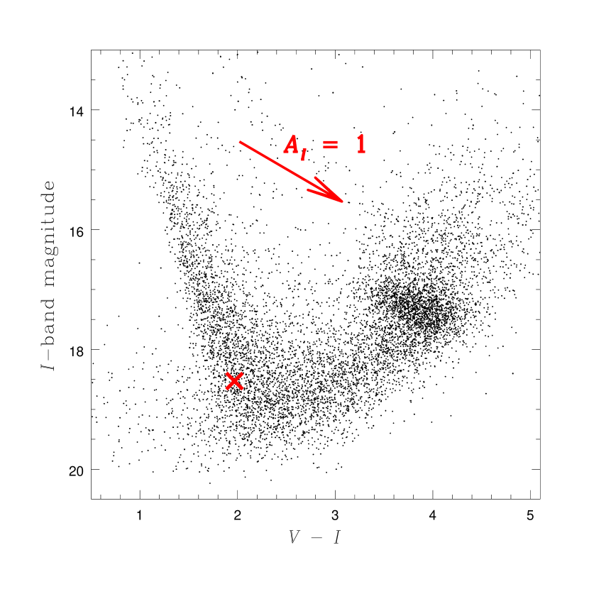
Figure 1: The colour-magnitude diagram for stars within 5 arcmin around sc5_2859. The position of the lensed star is denoted by a cross and the arrow denotes the reddening vector. From this figure it appears that the source is located in the main sequence branch and we believe that the source probably resides in the disk (see Section 4.1). The red clump giant region is clearly visible at $I\approx 17.4$, $(V-I)\approx 3.8$, which highlights that this field is subject to a large amount of interstellar extinction owing to the fact that the field of view is very close to the Galactic plane ($b\approx-1.5^{\circ}$ for sc5_2859). This figure was produced using the $VI$ photometric maps of the Galactic bulge presented in Udalski et al. (2002) and available online from http://bulge.princeton.edu/~ogle/ogle2/bulge_maps.html.

The baseline magnitude for the source is given by $I=18.53\pm 0.02$ mag, and the colour is $(V-I)=1.97\pm 0.02$ mag. In Fig. 1 we present the colour-magnitude diagram for the field around sc5_2859. From this figure it can be seen that the field around sc5_2859 is subject to a large amount of interstellar extinction, owing to the fact that the source is located very close to the Galactic plane. It appears that the lensed star is located in the main sequence branch of the colour-magnitude diagram. We will return to the issue of the possible source location and spectral type in Section 4.1.

3 Model fitting

We initially fit the event with the standard microlensing model, which assumes that the observer, lens and (point) source all move with constant velocities. The magnification is given by (see, for example, Paczyński 1986),

$$A(t)={u^{2}+2\over u\sqrt{u^{2}+4}},~{}~{}u(t)\equiv\sqrt{u_{0}^{2}+\tau(t)^{2}},$$ (1)

where $u_{0}$ is the impact parameter (in units of the Einstein radius) and,

$$\tau(t)={t-t_{0}\over t_{\rm E}},$$ (2)

with $t_{0}$ being the time of the closest approach (i.e., maximum, magnification), and $t_{\rm E}$ the event time-scale. The time-scale is defined such that,

$$t_{\rm E}={r_{\rm E}\over v}={\tilde{r}_{\rm E}\over\tilde{v}},$$ (3)

where $r_{\rm E}$ is the lens’ Einstein radius, $v$ is the lens’ transverse velocity relative to the observer-source line of sight, and $\tilde{r}_{\rm E}$ and $\tilde{v}$ are the values of these two quantities projected onto the observer plane. Therefore, $t_{\rm E}$ corresponds to the time it takes for the lens to move a distance equal to its Einstein radius.

The Einstein radius projected onto the observer plane is related to the mass according to the following equation,

$$\tilde{r}_{\rm E}=\sqrt{4GMD_{\rm S}x\over{c^{2}(1-x)}},$$ (4)

where $M$ is the lens mass, $D_{\rm S}$ the distance to the source and $x=D_{\rm L}/D_{\rm S}$ is the ratio of the distance to the lens and the distance to the source. This shows the well-known degeneracy inherent in the standard microlensing formalism; the quantities $\tilde{v}$, $M$ and $x$ cannot be determined uniquely from a given microlensing light curve, even if the source distance is known.

The Difference Image Analysis flux is given by,

$$F(t)=F_{0}\left(f_{\rm S}\left[A(t)-1\right]+1\right)-F_{\rm Ref},$$ (5)

where $F_{0}$ is the total baseline flux from the source plus any blended star(s), if present, $f_{\rm S}$ is the ratio of the baseline source flux to the total baseline flux (i.e. a measure of the blending), and $F_{\rm Ref}=416.15$ is the flux of the reference image. All the fluxes here are in units of 10 ADU and can be converted into $I$-band magnitudes using the following transformation (given in Woźniak et al. 2001),

$$I(t)=I_{\rm Ref}-2.5\,{\rm log}_{10}\frac{F(t)}{F_{\rm Ref}},$$ (6)

where $I_{\rm Ref}=16.76$ is the $I$-band magnitude of the reference image. Note that the reference image is brighter than the baseline magnitude for sc5_2859.

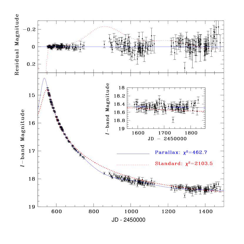
Figure 2: The I-band light curve for the OGLE-II event sc5_2859 from Difference Image Analysis. The best-fit standard and parallax models are given by the dotted and solid lines respectively. The upper panel shows the residual magnitude (the observed data points with the parallax model subtracted), and the inset shows the 4th season. Clearly the standard model is unable to reproduce the observed behaviour, but the parallax model provides a good fit with a $\chi^{2}$ per degree of freedom of 1.23.

We fit the light curve with the above five parameters for the standard model, i.e., $t_{0}$, $t_{\rm E}$, $u_{0}$, $F_{0}$, $f_{\rm S}$. The best-fit parameters are given in Table 1, and the corresponding light curve is shown in Fig. 2. Clearly this model is unable to provide a suitable fit for the data, with the best standard $\chi^{2}$ per degree of freedom greater than 5.

Table 1: The best standard model (first row) and the best parallax model (second row) for sc5_2859. The final column shows the $\chi^{2}$ and number of degrees of freedom (dof) for each model. The parameters are explained in Section 3.

Model	$t_{0}$	$t_{\rm E}$ (day)	$u_{0}$	$F_{0}$	$f_{\rm S}$	$\psi$ (radians)	$\tilde{r}_{\rm E}$ (au)	$\chi^{2}$/dof
S	$547.80\pm 0.20$	$815.4^{+7.5}_{-7.4}$	$-0.02767\pm 0.00028$	$70.17\pm 0.54$	$1.00000^{+0}_{-0.00042}$	—	—	2103.5 / 377
P	$542.20\pm 0.87$	$547.6^{+22.6}_{-7.8}$	$0.0645^{+0.0046}_{-0.0045}$	$81.83\pm 0.54$	$1.000^{+0}_{-0.065}$	$0.0477^{+0.0021}_{-0.0020}$	$10.84^{+0.44}_{-0.41}$	462.7 / 375

Since the duration of this event is longer than one year, the next logical step is to fit the light curve with a model that incorporates the parallax effect (Gould 1992). This effect, which arises when the Earth’s motion around the Sun is considered, is described in detail in Soszyński et al. (2001); see also Alcock et al. (1995), Dominik (1998). It requires two additional parameters, the Einstein radius projected onto the observer plane, $\tilde{r}_{\rm E}$, and an angle in the ecliptic plane, $\psi$, describing the orientation of the lens trajectory (given by the angle between the heliocentric ecliptic $x$-axis and the normal to the trajectory).

The parallax model produces a drastic reduction in $\chi^{2}$. The best-fit parameters are given in Table 1, and the corresponding light curve is shown in Fig. 2. The $\chi^{2}$ per degree of freedom is 1.23, which indicates that the parallax model provides a reasonable fit to the data.

We also fit this event with a slight variation on the above parallax model. In the above model we describe the geometrical properties in the ecliptic plane and then project these quantities into the lens plane. However, since the ecliptic plane intersects the Galactic bulge, this can lead to the projection being almost singular. Therefore, to avoid this potential singularity, one can instead take the more conventional approach and describe the geometrical properties in the plane perpendicular to the line-of-sight (see, for example, Dominik 1998, Alcock et al. 1995); to describe the lens plane coordinate system we form a right-handed set with the $x$-axis chosen to correspond to the North Ecliptic Pole projected onto the lens plane and the $z$-axis chosen to be the observer-source line-of-sight, which implies that the $y$-axis corresponds to the intersection of the lens plane and the Ecliptic plane. We find that the best-fit parameters are practically identical and therefore we do not present them here. However, for this coordinate system, the angle describing the relative lens-source trajectory is found to be $\theta=-35.96^{+0.66}_{-1.20}$ degrees, where $\theta$ is the angle between the trajectory and the $x$-axis (measured from the positive $x$-axis towards the positive $y$-axis).

From Table 1, the parallax parameters that provide information regarding the lens properties are,

$$\tilde{r}_{\rm E}=10.84^{+0.44}_{-0.41}~{}{\rm au},~{}~{}t_{\rm E}=547.6^{+22.6}_{-7.8}~{}{\rm days},$$ (7)

which implies that the transverse velocity of the lens relative to the source, projected onto the observer plane is,

$$\tilde{v}=\frac{\tilde{r}_{\rm E}}{t_{\rm E}}=34.2^{+1.5}_{-1.9}~{}\rm{kms}^{-1}.$$ (8)

If we convert the direction of $\tilde{v}$ from the lens plane ($\theta=-36.0$ degrees) into the plane perpendicular to the line-of-sight to the Galactic centre, we find that $\tilde{v}$ is directed almost parallel to the Galactic plane in the direction of rotation ($\theta_{\rm G}=-6.1^{+0.7}_{-1.2}$ degrees, where $\theta_{\rm G}$ is measured from the Galactic plane towards the North Galactic Pole). In this aspect sc5_2859 is similar to the strong parallax events presented in Bennett et al. (2002a), all of which had $-90^{\circ}<\theta_{\rm G}<0^{\circ}$.

This timescale of 548 days is the second longest time-scale ever identified (after the event OGLE-1999-BUL-32/MACHO-99-BLG-22; see Mao et al. 2001, Bennett et al. 2002b). In addition, the value of $\tilde{r}_{\rm E}$ is also unusually large, which implies that this event could be another black-hole microlens candidate (c.f. the three current black-hole microlens candidates, which have $\tilde{r}_{\rm E}=29.3,\,11.2~{}{\rm and}~{}8.7~{}{\rm au}$; see Agol et al. 2002). Using equation (4), the mass of the lens for this event is given by,

$$M=7.21M_{\odot}\left(\frac{\tilde{r}_{\rm E}}{\rm 10.84\,au}\right)^{2}\left(\frac{\pi_{\rm rel}}{0.5{\rm mas}}\right),~{}~{}\pi_{\rm rel}\equiv{{{\rm AU}\over D_{\rm L}}-{{\rm AU}\over D_{\rm S}}}.$$ (9)

A value of $\pi_{\rm rel}=0.5$ mas corresponds to a disk source with $D_{\rm S}=2\,{\rm{kpc}}$ and $D_{\rm L}/D_{\rm S}=0.5$. There are various approaches that can be employed to constrain the location of the source and lens, and hence the lens mass; these are considered in Section 4.

To verify the viability of our parallax fit, we proceed to fit the event with a model that incorporates a constant acceleration term, instead of the Earth’s centripetal acceleration (see Smith, Mao & Paczyński 2003). This model is unable to provide a feasible fit for sc5_2859, meaning that the parallactic nature of the deviations appears to be secure.

4 Constraints on the lens mass

4.1 Finite-source effects

Since the peak magnification is predicted to be greater than 40, one may suspect that this event could be affected by finite-source effects (Gould 1994; Witt & Mao 1994; Nemiroff & Wickramasinghe 1994). Such effects become apparent when the lens passes sufficiently close to the source, resulting in an invalidation of the assumption that the source is point-like. However, there is one significant drawback for sc5_2859, namely that there is no coverage for the peak of the light-curve, i.e. the point at which the lens and source are in closest alignment and therefore where the finite-source effects should be most prominent.

To implement the finite-source model requires an additional parameter, $\rho_{\ast}$, which denotes the source radius in units of the lens’ angular Einstein radius. Despite the lack of coverage around the peak, constraints can be placed on $\rho_{\ast}$,

$$\rho_{\ast}<0.0418~{}~{}\mbox{at the 3$\sigma$ confidence level}.$$ (10)

This constraint on $\rho_{\ast}$ can be used to place a lower-limit on the mass of the lensing object. To do this, we first require an estimate of the angular size of the source star. From the colour-magnitude diagram presented in Fig. 1, it appears that the source lies on the main-sequence branch. The extinction and reddening for typical bulge stars in this field can be estimated from the position of the red clump region on the observed colour-magnitude diagram (see, for example, Albrow et al. 2000). The location of the centre of the red clump region for this field is given by $(V-I)_{\rm cl,obs}\approx 3.82$ mag. Since the intrinsic dereddened colour of the red-clump region is $(V-I)_{\rm cl,0}\approx 1.00$ mag (Popowski 2000), this implies that the clump is reddened by $E(V-I)_{\rm cl}\approx 2.82$ mag. The slope of the reddening line for this field ($A_{I}/E[V-I]=0.95$ for $l=0.1^{\circ}$, $b=-1.8^{\circ}$, Udalski 2002), yields the extinction for the red clump region, $A_{I,{\rm cl}}\approx 2.68$ mag. Therefore a star located in the red clump region, i.e. in the Galactic bulge, will undergo extinction and reddening of,

$$A_{I,{\rm cl}}\approx 2.68~{}{\rm mag},~{}~{}E(V-I)_{\rm cl}\approx 2.82~{}{\rm mag}.$$ (11)

In Section 2 we stated that the observed magnitude and colour of sc5_2859 is $I_{\rm obs}\approx 18.5$ mag and $(V-I)_{\rm obs}\approx 1.97$ mag. Since the best-fit parallax model presented in Section 3 predicts that there is no blending ($f_{\rm S}=1.000^{+0}_{-0.065}$, i.e. all of the observed flux comes from the source), this implies that the observed magnitude and colour of the source is $I_{\rm S,obs}\approx 18.5$ mag and $(V-I)_{\rm S,obs}\approx 1.97$ mag. Therefore, if the source were located in the bulge (with $D_{\rm S}\approx 8$ kpc) and underwent the same amount of reddening and extinction as given in equation (11), the absolute magnitude and intrinsic colour would be $M_{I}\approx 1.3$ mag and $(V-I)_{\rm S,0}\approx-0.85$ mag. However, this is clearly incompatible with spectral types known to be in the bulge. Therefore, we conclude that the source is unlikely to be a Galactic bulge star, i.e., sc5_2859 is more-likely an example of disk-disk lensing. By taking a simple model for the extinction we can obtain the absolute magnitude and colour of the source as a function of $D_{\rm S}$. We model the extinction using an exponential dust sheet of scale height 130pc (e.g. Drimmel & Spergel 2001), with the Sun located 20pc above the Galactic plane (Humphreys & Larsen 1995). This simple analysis suggests that the source is consistent with a K- or G-type dwarf at a distance of approximately $1.5-2.5$ kpc. For example, for $D_{\rm S}\approx 2.0$ kpc, this gives $M_{I,{\rm S}}\approx 6.0$, $I_{\rm S,0}\approx 17.5$ and $(V-I)_{\rm S,0}\approx 0.86$, with $A_{I}\approx 1.1$ mag.

We can check this conclusion by utilising a different approach. If we assume that the source is a typical G5 main-sequence star with absolute magnitude $M_{I}=4.41$ mag and $(V-I)_{\rm C}=0.69$ mag (from Cox 2000, converted into the Cousins system using Bessell 1979), then, given the slope of the reddening line for this field $A_{I}/E[V-I]=0.95$ (Udalski 2002), we can calculate the predicted source distance. This method suggests that $D_{\rm S}\approx 3.8$ kpc and $A_{I}\approx 1.2$ mag. Applying the same approach to a fainter K5 main-sequence star with $M_{I}=6.09$ mag and $(V-I)_{\rm C}=1.26$ mag (from Cox 2000) suggests that $D_{\rm S}\approx 2.3$ kpc and $A_{I}\approx 0.7$ mag.

Clearly, the exact brightness and colour of the source will vary depending on the assumptions; for the following analysis we shall proceed with the values calculated above using the simple extinction model and taking $D_{\rm S}\approx 2.0$ kpc. Spectroscopic observations of the source would be very useful to determine its spectral-type and hence constrain the distance to the source.

Our prediction for the intrinsic brightness and colour of the source can be used to estimate its angular size through an available empirical relationship. For example, van Belle (1999) provides the following relationship for B- to G-type main-sequence stars with $-0.4<(V-K)_{0}<+1.5$ mag,

$$\rm{log}~{}(2\theta_{\ast})+\frac{V_{\rm S,0}}{5}=0.500\pm 0.023+(0.264\pm 0.012)\times[(V-K)_{\rm S,0}].$$ (12)

The source star’s intrinsic colour of $(V-I)_{\rm S,0}\approx 0.86$ can be converted into $(V-K)_{\rm S,0}\approx 1.91$ (by using, for example, Table II of Bessell & Brett 1988), which implies the star’s angular radius is,

$$\theta_{\ast}\approx 1.08~{}\mu\rm{as},$$ (13)

If the distance to the source is $\sim 2.0$ kpc, this corresponds to a physical source radius of $\sim 0.5R_{\odot}$, i.e. slightly less than typical K- or G-type dwarfs (e.g. Table 15.8 of Cox [2000] gives the physical radius of K- and G-type dwarfs to be between $0.72R_{\odot}$ and $1.1R_{\odot}$).

This value for $\theta_{\ast}$ can be used to estimate the $3\sigma$ lower limit on the lens mass through the formula,

$$M=c^{2}(4G)^{-1}\tilde{r}_{\rm E}\theta_{\rm E},$$ (14)

since the lens’ angular Einstein radius is given by $\theta_{\rm E}=\theta_{\ast}/\rho_{\ast}$. Using the $\rho_{\ast}$ constraint provided in equation (10) gives,

$$M>0.034\,M_{\odot}~{}~{}\mbox{at the 3$\sigma$ confidence level},$$ (15)

which corresponds to $x=D_{\rm L}/D_{\rm S}<0.995$.

Therefore we are only able to place a weak lower-limit on the lens mass from finite-source considerations. This outcome can be understood when one considers the likely values of the parameter $\rho_{\ast}$. From equation (14), we can obtain the following relation for $\rho_{\ast}$,

$$\rho_{\ast}=0.003\left(\frac{\tilde{r}_{\rm E}}{10.84\,\rm{au}}\right)\left(\frac{R_{\ast}}{R_{\odot}}\right)\left(\frac{D_{\rm S}}{2.0\,\rm{kpc}}\right)^{-1}\left(\frac{M}{M_{\odot}}\right)^{-1},$$ (16)

where $R_{\ast}$ is the physical source radius, which we expect to be $\sim 1R_{\odot}$ if the source for sc5_2859 is a main-sequence star. Gould (1994) showed that the detection of finite-source signatures is only possible provided $\rho_{\ast}>1/A_{\rm max}$, where $A_{\rm max}$ is the peak magnification. For sc5_2859 we have $1/A_{\rm max}\approx 0.023$, which implies that finite-source signatures are extremely unlikely to be detected.

4.2 Additional considerations regarding the lens mass

In addition to the above weak constraint placed on the lens mass from the finite-source analysis, there is other information that we can use from the properties of the best-fit parallax model, i.e. independent of the above finite-source fit. First, we shall consider the parallax velocity parameter ($\tilde{v}$), and then incorporate our knowledge of the limits on the blended flux.

For parallax microlensing events the velocity parameter $\tilde{v}$ (i.e. the transverse velocity of the lens relative to the source, projected onto the observer plane), must be sufficiently small so that the Earth’s orbital motion is able to affect the light curve. For sc5_2859, this transverse velocity is $\tilde{v}=34.2^{+1.5}_{-1.9}~{}\rm{kms}^{-1}$ directed almost parallel to the Galactic plane in the direction of rotation ($\theta_{\rm G}=-6.1$ degrees; see Section 3). The velocity vector $\tilde{\bf v}$ is related to the transverse velocities of the observer (i.e. the Sun, ${\mathbf{v}}_{\odot}$), source (${\mathbf{v}}_{\rm S}$) and lens (${\mathbf{v}}_{\rm L}$), where ${\mathbf{v}}_{\odot}$, ${\mathbf{v}}_{\rm S}$ and ${\mathbf{v}}_{\rm L}$ are the 2-dimensional velocities perpendicular to the line-of-sight (i.e. in the lens plane), through the equation,

$$\tilde{\mathbf{v}}=\frac{{\mathbf{v}}_{\rm L}-x{\mathbf{v}}_{\rm S}}{1-x}-{\mathbf{v}}_{\odot}.$$ (17)

Previous studies of parallax microlensing events (e.g. Alcock et al. 1995) have used the parameter $\tilde{\bf v}$ and equation (17) to obtain a likelihood function for $x$ (and hence, from equation [4], a likelihood function for the lens mass),

$$L(x;\tilde{\bf v})\propto\sqrt{x(1-x)}\,\rho_{\rm L}(x)\,|\tilde{\bf v}|\,(1-x)^{3}\,\int f_{\rm v,S}({\bf v}_{\rm S})\,f_{\rm v,L}([1-x][{\bf v}_{\odot}+\tilde{\bf v}]+x{\bf v}_{\rm S})\,d{\bf v}_{\rm S},$$ (18)

where $f_{\rm v,L}$ and $f_{\rm v,S}$ are the lens and source velocity distributions, $\rho_{\rm L}(x)$ is the density of lenses at a distance $x$, and all vectors are described in the plane perpendicular to the line-of-sight to the Galactic centre (i.e. two dimensional). A more thorough analysis may be obtained by including a mass function prior (see, for example, Agol et al. 2002). However, we do not attempt such an analysis here; for the purposes of this work we follow the approach of Bennett et al. (2002b) and assert that the likelihood function represents all of our knowledge about the lens mass and location (i.e. we select a uniform prior), meaning that the above likelihood function can be interpreted as the probability distribution for $x$.

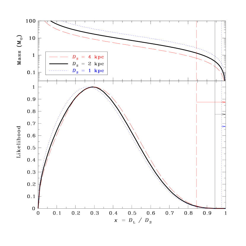
Figure 3: Bottom Panel: The likelihood function for $x=D_{\rm L}/D_{\rm S}$ given the observed parallax velocity parameter ($\tilde{v}=34.2$ km/s in a direction $\theta_{\rm G}=-6.1^{\circ}$) for event sc5_2859. As well as the preferred value of $D_{\rm S}\approx 2.0$ kpc (see Section 4.1), two additional values are presented for comparison. The vertical lines represent the $2\sigma$ lower limits on $x$ for each value of $D_{\rm S}$; these constraints are found by considering the upper limits on the lens luminosity, assuming that the lens is a main-sequence star (see Section 4.2). Top Panel: This shows how the lens mass varies with $x$ for each value of $D_{\rm S}$.

We evaluate this function by assuming that both the lens and source reside in the disk, using density and mass distributions from Belokurov & Evans (2002) and taking the Sun’s two dimensional peculiar velocity to be 8.89 km/s in a direction $\theta_{\rm G}=53.8^{\circ}$ (Dehnen & Binney 1998). The results of this calculation are presented in Figure 3. From this figure, we can see that the distribution for $x$ is not very narrow, implying that the lens can take a wide range of masses. For example, for $D_{\rm S}\approx 2.0$ kpc, this analysis suggests that $x=0.32^{+0.20}_{-0.17}$ and hence the lens mass $M=15.6^{+27.4}_{-8.8}M_{\odot}$; moreover, the $2\sigma$ lower limit on the lens mass is $3.1M_{\odot}$, suggesting that a low mass lens is strongly disfavoured.

Additional constraints can be placed on the lens nature by considering the blended flux parameter, $f_{\rm S}$. The best-fit parallax model given in Section 3 predicts that there is no blending (i.e., $f_{\rm S}=1$), meaning that all of the flux is being emitted by the lensed source. This is important because it suggests that the lens may not be a main sequence star, since if this was true one would expect some blending due to the light from the lens, i.e. one would expect $f_{\rm S}<1$.

This possibility can be investigated by considering the limits on the $f_{\rm S}$ parameter. From the best-fit parallax model, we can say that the $2\sigma$ and $3\sigma$ limits on the lens brightness are $I_{\rm L,obs}>20.14$ and $I_{\rm L,obs}>19.62$, respectively. If we model the lens with a main-sequence mass-luminosity relation $L\propto M^{4}$, we can use this to place a lower limit on $x$ through equation (4). However, to do this we need to know the source distance, $D_{\rm S}$, and also how the extinction varies with distance. If we again take $D_{\rm S}\approx 2.0$ kpc and assume the previous simple extinction model (see Section 4.1), we obtain $2\sigma$ and $3\sigma$ limits of $x>0.944$ and $x>0.937$, respectively. This conclusion depends only weakly on the assumptions regarding the extinction and mass-luminosity relation. These constraints on $x$ appear to contradict the above conclusions from the $\tilde{v}$ likelihood analysis, which suggested that values of $x$ close to 1 are strongly disfavoured due to the low value of $\tilde{v}$. Figure 3 shows how the $2\sigma$ limits on the lens brightness compare to the likelihood distribution described in equation (18) for three values of $D_{\rm S}$. These constraints appear to be incompatible with the above likelihood analysis (for example, for $D_{\rm S}=2.0$ kpc, the likelihood analysis gives the probability that $x$ satisfies the $2\sigma$ constraints on the lens brightness to be $<10^{-4}$).

Therefore, we tentatively conclude that the lens for sc5_2859 is unlikely to be a main-sequence star, which implies that this event could be a white dwarf (although this seems unlikely, given that typical white dwarf masses of $\la 1M_{\odot}$ [Bergeron, Ruiz, & Leggett 1997] are disfavoured from our likelihood analysis), a neutron star, or possibly an example of lensing by a stellar mass black hole (Agol et al. 2002; Bennett et al. 2002a).

5 Discussion

5.1 The nature of event sc5_2859

One approach that can be utilised to probe the nature of the lens for sc5_2859 is through proper motion analysis. If the proper motion of the source can be measured, then this can be combined with the parallax model’s prediction for the transverse velocity of the lens relative to the source (i.e. $\tilde{v}$) to determine the proper motion of the lens. The importance of this method is that it can be applied even in the case where the lens is not luminous. By analysing one OGLE-II field, Sumi, Eyer & Woźniak (2003) have shown that proper motion measurements can be determined for objects in the OGLE-II catalogue. Preliminary results from the analysis of all OGLE-II fields suggests that the source star for sc5_2859 may have a large proper motion (Sumi, private communication), although this requires verification as the source star is relatively faint.

Despite the fact that the light curve for sc5_2859 appears to be reasonably well fit by the parallax microlensing model (see Section 3), it is not inconceivable that the variation in brightness could be due to some phenomena other than microlensing. Whilst this ambiguity can affect any microlensing event, for sc5_2859 it is particularly severe since data only exist for the declining branch of the light curve. Indeed, recently Cieslinski et al. (2003) carried out a search of OGLE-II light curves in an attempt to identify new cataclysmic variables. In this work they suggested that the shape of the light curve for sc5_2859 indicates that this event could be a candidate nova. However, it is known that microlensing events, unlike many intrinsically variable stars, are expected to be achromatic (this may not be true for heavily blended events, but for sc5_2859 the best-fit model predicts no blended flux). For sc5_2859 the OGLE data only provide colour information for two epochs, namely ${\rm JD}-2450000\approx 608$ days, and ${\rm JD}-2450000\approx 1020$ days. Reassuringly, the $(V-I)$ colour appears to stay roughly constant for these two epochs, with $(V-I)=1.97\pm 0.02$ and $(V-I)=2.06\pm 0.07$, respectively, which supports our belief that sc5_2859 is a microlensing event.

5.2 Scientific returns from long duration events such as sc5_2859

An important aspect of sc5_2859 that is worth noting is that the above analysis is possible even though data exist for less than half of the microlensing light curve. Despite the fact that observations commenced after the peak, it is still possible to identify the parallactic signatures and gain well-constrained measurements of $\tilde{r}_{\rm E}$ and $\theta$. Obviously, this is only possible for sc5_2859 due to the high-quality data and the long duration of the event. In future, even with initially sparse sampling, long-duration events can provide useful information provided high-quality data are obtained for the latter part of the light curve. This highlights the importance of real-time microlensing alert systems (such as the OGLE-III Early Warning System or the MOA Transient Alert Page) and also the importance of high-quality follow-up observations (such as those performed by the PLANET collaboration).

On the other hand, if real-time alert systems can detect events at a suitably early stage, then it could be possible to make direct determinations of the lens mass. For example, once the ESO Very Large Telescope Interferometer becomes fully operational, its high sensitivity may enable measurements to be made of the angular separation of the two microlensed images (Delplancke, Górski & Richichi 2001). Coupled with a measurement of the parallax effect, this would completely break the lens degeneracy and unambiguously determine the mass of the lensing object. In future this approach could prove to be very important for long-duration microlensing events.

Another approach that would benefit from timely follow-up observations is the method of combining the parallax model with finite-source effects. As was shown in Section 4.1, if firm measurements can be made of both parallax and finite-source effects, is it possible to completely break the lens degeneracy and determine the lens mass. Although this was not possible for sc5_2859, it has recently been shown to be feasible (for example, this approach was applied to the OGLE-II event sc26_2218, resulting in a tentative lens mass determination [Smith, Mao & Woźniak 2003]). If real-time alert systems are able to identify high-magnification long-duration events suitably early, it may be possible to obtain good quality data for the peak of the light curve and hence determine the lens mass.

5.3 An excess of long-duration events in OGLE-II?

With the addition of sc5_2859, this brings the total number of known events in the OGLE-II catalogue with $t_{\rm E}>1$ year to three: OGLE-1999-BUL-32 ($t_{\rm E}=640^{+68}_{-54}$ days; Mao et al. 2002), sc5_2859 ($t_{\rm E}=547.6^{+22.6}_{-7.8}$ days; see Section 3 above), and OGLE-1999-BUL-19 ($t_{\rm E}=372.0\pm{3.3}$ days; Smith et al. 2002). Information regarding these three events is presented in Table 2.

Table 2: The three longest-duration events in the OGLE-II catalogue. The fit parameters are derived from the best-fit parallax model to the OGLE-II Difference Image Analysis data (Woźniak et al. 2001). The parameters $t_{\rm E}$, $\tilde{r}_{\rm E}$ and $f_{\rm S}$ are defined in Section 3, $I_{0}$ is the total $I$-band baseline magnitude of the source plus any blended star(s), if present, and $A_{\rm max}$ is the peak magnification (predicted from the best-fit parallax model). Event OGLE-1999-BUL-32 was also detected by the MACHO collaboration (by which it was named MACHO-99-BLG-22) and they find $t_{\rm E}=560\pm 45$ days and $\tilde{r}_{\rm E}=24.3\pm 3.5$ au (Bennett et al. 2002b).

Name	$t_{\rm E}$ (day)	$\tilde{r}_{\rm E}$ (au)	$I_{0}$	$f_{\rm S}$	$A_{\rm max}$	RA (J2000)	Dec (J2000)	Reference
OGLE-1999-BUL-32	$640^{+68}_{-54}$	$29.1^{+6.4}_{-5.4}$	18.1	0.37	31.8	18:05:05.35	-28:34:42.5	Mao et al. (2002)
sc5_2859	$547.6^{+22.6}_{-7.8}$	$10.84^{+0.44}_{-0.41}$	18.5	1.00	43.9	17:50:36.09	-30:01:46.6	Section 3
OGLE-1999-BUL-19	$372.0\pm{3.3}$	$2.68\pm 0.02$	16.1	0.82	10.2	17:51:10.76	-33:03:44.1	Smith et al. (2002)

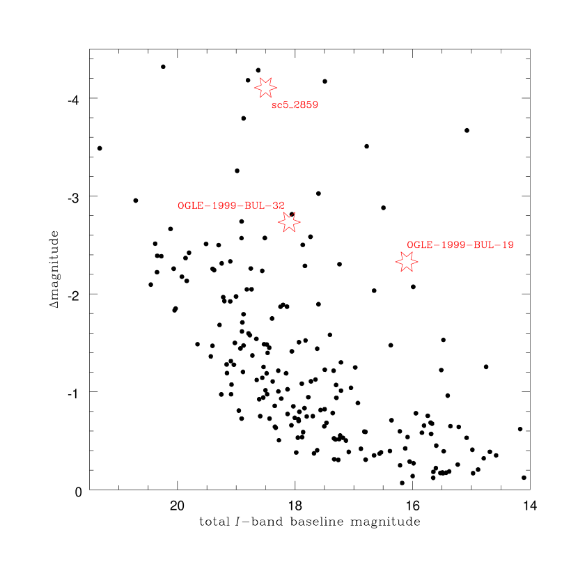
Figure 4: The total $I$-band baseline magnitude vs the change in magnitude at peak magnification (as predicted by the best-fit standard model) for a high-quality 257-event subset of the OGLE-II Difference Image Analysis catalogue (Woźniak et al. 2001). The three longest-duration events are denoted by the star symbols (for these events the change in magnitude is based on the best-fit parallax model). Since the change in magnitude is based on a model fit, it is possible that for some events (i.e. those for which the peak magnification is not covered by the data) the predicted change in magnitude may be unreliable. The lack of events in the lower-left of the diagram is to be expected and is simply due to the OGLE-II detection limit. It appears that these three longest-duration events do not lie within the main cluster of events and this could have important implications for the abundance of such long-duration events (see Section 5.3).

Table 2 shows that these three OGLE-II events are all highly magnified, with peak magnifications ranging from 10.2 to greater than 40. Figure 4 illustrates how these magnifications compare to a high-quality subset of the OGLE-II catalogue. By plotting the total baseline magnitude vs the change in magnitude at peak magnification, it can clearly be seen that these three events do not appear to lie within the main cluster. This could suggest that some, if not all, of these three long duration events are artifacts, i.e. the variability may not be due to microlensing. However, we believe that this is more-likely due to a selection effect, which implies that there could be additional long-duration events residing in the main lower-magnification cluster, i.e., events that have been omitted from existing OGLE-II microlensing catalogues due to insufficient magnification (low signal-to-noise ratio). In addition, from this table it is interesting to note that that these events do not appear to be clustered in any one direction (c.f. Popowski 2002, where it is claimed that an abundance of long duration MACHO events appear to be clustered in one particular direction).

Previous work has indicated the existence of an excess of long duration microlensing events toward the Galactic bulge (e.g., Han & Gould 1996; Zhao, Rich & Spergel 1996; Bennett et al. 2002a). However, is it possible to quantify the extent to which these three longest-duration OGLE-II events constitute an excess? If one naïvely extrapolates the behaviour of the timescale distribution of moderately long duration OGLE-II events to long timescales using a $t_{\rm E}^{-3}$ power-law (Mao & Paczyński 1996), this predicts far fewer than three events should have $t_{\rm E}>1$ year. However, to perform this calculation thoroughly requires the detection efficiency of the OGLE-II catalogue, which is currently undetermined. We aim to investigate this important issue and report our findings in a future paper.

One implication of this potential excess is that many long-duration events could easily be overlooked by microlensing search projects. Microlensing detection algorithms usually rely on the presence of a constant baseline to differentiate true events from variable stars. However, such long-duration events may exhibit noticeable magnification over the course of many years, which can mean that a constant baseline is not observed. For example, the detection algorithm of Woźniak et al. (2001) initially failed to identify the three longest-duration events (i.e., those presented in Table 2) owing to the fact that they did not pass the constant-baseline criteria. These three events were only found when this OGLE-II catalogue was compared with a previous, independently constructed, catalogue of OGLE-II events. Also, as was mentioned above, it is conceivable that there are additional long-duration events in the OGLE-II catalogue that have been omitted due to having insufficient magnification (i.e., low signal-to-noise ratio). However, it should be noted that if some long-duration events are being overlooked in microlensing catalogues then this would increase the observed optical depth, which is already significantly larger than current theoretical predictions (see, for example, Binney, Bissantz & Gerhard 2000; Evans & Belokurov 2002; Klypin, Zhao & Somerville 2002).

6 Conclusion

This paper has presented a new long-duration parallax event from the OGLE-II database, sc5_2859, which has $t_{\rm E}=547.6^{+22.6}_{-7.8}$ days. We believe that both the lens and source reside in the Galactic disk, making event sc5_2859 one of the first confirmed examples of so-called disk-disk lensing. In this aspect it differs from the two other longest-duration events, which are both believed to have source stars located in the Galactic bulge (Mao et al. 2002, Bennett et al. 2002b; Smith et al. 2002).

The source star for sc5_2859 is likely to be located at a distance of $D_{\rm S}\sim 2.0$ kpc, although we are not able to provide a definitive value (see Section 4.1). This is the major source of uncertainty in the analysis presented in Section 4. We strongly recommend that spectroscopic observations of the source are carried out in order to determine the spectral-type of the source and hence improve the estimate of $D_{\rm S}$.

In Section 4.2 we showed that the transverse velocity of the lens relative to the source ($\tilde{v}$) can be used to construct a likelihood function for $x=D_{\rm L}/D_{\rm S}$ and hence the lens mass. This analysis suggests that lens is unlikely to be a main-sequence star, since the resulting luminosity of the lens would exceed the limits imposed on the blended flux from the parallax model. Therefore sc5_2859 could be another candidate for microlensing by a stellar mass black hole (Agol et al. 2002; Bennett et al. 2002a).

Note added in proof

After this paper was accepted for publication, it was discovered that the EROS microlensing collaboration also observed the field of sc5_2859 during this event. Preliminary analysis of these data suggest that they are in good agreement with the OGLE-II data during the period when the observations overlapped. However, there are a number of EROS data-points prior to the beginning of the OGLE-II observations (i.e. for the period $\rm{JD}-245000<550$ d), and these data appear to be incompatible with the microlensing model presented in this paper. It is hoped that the definitive analysis of the EROS data, when combined with relevant follow-up observations, will help to clarify the nature of this event. The results of these findings will be presented at a later date.

References

- [1] Agol E., Kamionkowski M., Koopmans L., Blandford R. 2002, ApJ, 576, L131
- [2] Alard C., Lupton R. H., 1998, ApJ, 503, 325
- [3] Albrow M. D., et al., 2000, ApJ, 534, 894
- [4] Alcock C., et al., 1995, ApJ, 454, L125
- [5] Alcock C., et al., 2000, ApJ, 541, 734 (erratum 557, 1035 [2001])
- [6] Afonso C. et al. (The EROS collaboration), 2003, A&A, 404, 145
- [7] Becker A.C., 2000, PhD thesis, University of Washington
- [8] van Belle G.T., 1999, PASP, 111, 1515
- [9] Belokurov V., Evans N.W., 2002, MNRAS, 331, 649
- [10] Bennett D.P., et al. 2002a, ApJ, 579, 639
- [11] Bennett D.P., Becker A.C., Calitz J.J., Johnson B.R., Laws C., Quinn J.L., Rhie S.H., Sutherland W., 2002b, (astro-ph/0207006)
- [12] Bergeron P., Ruiz M. T., Leggett S. K., 1997, ApJS, 108, 339
- [13] Bessell M. S., 1979, PASP, 91, 589
- [14] Bessell M. S., Brett J. M., 1988, PASP, 100, 1134
- [15] Binney J., Bissantz N., Gerhard O., 2000, ApJ, 537, L99
- [16] Cieslinski D., Diaz M.P., Mennickent R.E., Pietrzyński G., 2003, PASP, 115, 193
- [17] Cox A., 2000, Allen’s Astrophysical Quantities (4th Edition), Springer-Verlag, New York
- [18] Dehnen W., Binney J.J., 1998, MNRAS, 298, 387
- [19] Delplancke F., Górski K. M., Richichi A., 2001, A&A, 375, 701
- [20] Dominik M., 1998, A&A, 329, 361
- [21] Drimmel R., Spergel D.N., 2001, ApJ, 556, 181
- [22] Evans N.W., Belokurov V., 2002, ApJ, 567, L119
- [23] Gould A., 1992, ApJ, 392, 442
- [24] Gould A., 1994, ApJ, 421, L71
- [25] Han C., Gould A., 1996, ApJ, 467, 540
- [26] Humphreys R.M., Larsen J.A., 1995, AJ, 110, 2183
- [27] Klypin A., Zhao H.S., Somerville R., 2002, ApJ, 573, 597
- [28] Mao S., Paczyński B., 1996, ApJ, 473, 57
- [29] Mao S., Smith M.C., Woźniak P., Udalski A., Szymański M., Kubiak M., Pietrzyński G., Soszyński I., Żebruń K., 2002, MNRAS, 329, 349
- [30] Nemiroff R.J., Wickramasinghe W.A.D.T., 1994, ApJ, 424, L21
- [31] Paczyński B., 1986, ApJ, 304, 1
- [32] Paczyński B., 1996, ARAA, 34, 419
- [33] Peale S.J., 1998, ApJ, 509, 177
- [34] Popowski, P. 2000, ApJ, 528, L9
- [35] Popowski P., 2002, submitted to MNRAS (astro-ph/0205044)
- [36] Rhie S.H., Becker A.C., Bennett D.P., Fragile P.C., Johnson B.R., King L.J., Peterson B.A., Quinn J., 1999, ApJ, 522, 1037
- [37] Schechter P.L., Mateo M., Saha A., 1993, PASP, 105, 1342
- [38] Smith M. C. et al. 2002, MNRAS, 336, 670
- [39] Smith M.C., Mao S., Paczyński B., 2003, MNRAS, 339, 925
- [40] Smith M.C., Mao S., Woźniak P., 2003, ApJL, 585, 65
- [41] Soszyński I. et al. 2001, ApJ, 552, 731
- [42] Sumi T. et al., 2002, submitted to ApJ(astro-ph/0207604)
- [43] Sumi T., Eyer L., Woźniak P., 2003, submitted to MNRAS (astro-ph/0210381)
- [44] Udalski, A. 2002, astro-ph/0210367
- [45] Udalski A., Szymański M., Kałużny J., Kubiak M., Krzemiński W., Mateo M., Preston G.W., 1993, Acta Astron., 43, 289
- [46] Udalski A., Kubiak M. & Szymański M., 1997, Acta Astron., 47, 319
- [47] Udalski A., Żebruń K., Szymański M., Kubiak M., Pietrzyński G., Soszyński I., Woźniak P., 2000, Acta Astron., 50, 1
- [48] Udalski A., Szymański M., Kubiak M., Pietrzyński G., Soszyński I., Woźniak P., Żebruń K., Szewczyk O., Wyrzykowski Ł., 2002, Acta Astron., 52, 217
- [49] Woźniak P., Udalski A., Szymański M., Kubiak M., Pietrzyński G., Soszyński I., Żebruń K., 2001, Acta Astron., 51, 175
- [50] Witt H.J., Mao S., 1994, ApJ, 430, 505
- [51] Zhao H.S., Rich R.M., Spergel D.N., 1996, MNRAS, 282, 175