Weak Lensing from Space II:
Dark Matter Mapping

Abstract

We study the accuracy with which weak lensing measurements could be made from a future space-based survey, predicting the subsequent precisions of 3-dimensional dark matter maps, projected 2-dimensional dark matter maps, and mass-selected cluster catalogues. As a baseline, we use the instrumental specifications of the Supernova/Acceleration Probe (SNAP) satellite. We first compute its sensitivity to weak lensing shear as a function of survey depth. Our predictions are based on detailed image simulations created using ‘shapelets’, a complete and orthogonal parameterization of galaxy morphologies. We incorporate a realistic redshift distribution of source galaxies, and calculate the average precision of photometric redshift recovery using the SNAP filter set to be $\Delta z=0.034$. The high density of background galaxies resolved in a wide space-based survey allows projected dark matter maps with a rms sensitivity of 3% shear in 1 arcmin² cells. This will be further improved using a proposed deep space-based survey, which will be able to detect isolated clusters using a 3D lensing inversion techniques with a 1$\sigma$ mass sensitivity of approximately $10^{13}M_{\odot}$ at $z=0.25$. Weak lensing measurements from space will thus be able to capture non-Gaussian features arising from gravitational instability and map out dark matter in the universe with unprecedented resolution.

1 Introduction

Weak gravitational lensing has now been established as a powerful technique to directly measure the large-scale mass distribution in the universe (for reviews, see Mellier 1999; Bartelmann & Schneider 2001; Refregier 2003). Several groups have measured the coherent distortion of background galaxy shapes around known galaxy clusters (e.g. Joffre et al. 2000; Dahle et al. 2002) and also statistically in the field (e.g. van Waerbeke et al. 2001; Bacon et al. 2002; Hoekstra et al. 2002; Jarvis et al. 2003). Ever-growing surveys using ground-based telescopes are beginning to yield useful constraints on cosmological parameters (Bacon et al. 2003; Brown et al. 2002; Hoekstra, Yee, & Gladders 2002; van Waerbeke et al. 2002). The first two clusters selected purely by weak lensing mass have now been found and spectroscopically confirmed by Wittman et al. (2001, 2003).

Weak lensing is of such great interest for cosmology because it is directly sensitive to mass. Other observations have traditionally been limited to measuring the distribution of light and linked to theory via complications like the mass-temperature relation for $x$-ray selected clusters (Pierpaoli, Scott & White 2001; Viana, Nicholl & Liddle 2002; Huterer & White 2003) or the ubiquitous problem of bias (Weinberg et al. 2003). Weak lensing measurements first avoid these problems, then have even been used to calibrate other techniques (Huterer & White 2003; Gray et al. 2002; Hoekstra et al. 2002b; Smith et al. 2003). The high resolution, galaxy number density and stable image quality available from space-based weak lensing data will allow maps of the projected distribution of dark matter to be reconstructed at unprecedented resolution. The mass power spectrum can be sliced into multiple redshift bins using photometric redshifts: providing a long lever arm for constraints on the evolution of cosmological parameters. Even three-dimensional mass maps, marginally feasible from the ground (Bacon & Taylor 2002), are likely to be sensitive to overdensities as small as galaxy groups from space.

Mass-selected cluster catalogs can also be extracted from such maps (Weinberg & Kamionkowski 2002, Hoekstra 2002). Cluster counts, and the quantitative study of high-sigma density perturbations or higher order shear correlation functions (Bernardeau, van Waerbeke & Mellier 1997; Cooray, Hu & Miralda-Escudé 2000; Munshi & Jain 2001; Schneider & Lombardi 2003) are one of the most promising routes to breaking degeneracies in the estimation of cosmological parameters including $\Omega_{\rm m}$ and $w$, the dark energy equation of state parameter. Furthermore, studying well-resolved groups and clusters individually, rather than statistically, will lead to a better understanding of astrophysical phenomena, the nature of dark matter and the growth of structure under the gravitational instability paradigm (e.g. Dahle et al. 2003).

In this paper, we predict the general sensitivity to weak lensing of a space-based wide field imaging telescope, taking as a baseline the specifications of the proposed Supernova/Acceleration Probe (SNAP) satellite. Instrument characteristics, including the PSF, ellipticity patterns and image stability have been studied by Rhodes et al. (2003; paper I). In $\S\ref{sims}$ we introduce detailed simulated images that have been developed using shapelets, an orthogonal parameterization of galaxy shapes (Massey et al. 2003, Refregier 2003). The simulated images contain realistic populations and morphologies of galaxies as will be seen from space, modelled from those in the Hubble Deep Fields (HDFs; Williams et al. 1996, 1998). These shapelet-galaxies can be artificially sheared to simulate gravitational lensing. The subsequent recovery accuracy of the known input shear is discussed in $\S\ref{sens}$. We discuss the accuracy of SNAP photometric redshifts in $\S\ref{photoz}$. These two measurements are combined to predict the accuracy of projected dark matter maps, 3-dimensional dark matter maps and mass-selected cluster catalogues in $\S\ref{maps}$. We draw conclusions in $\S\ref{conc}$. Our results are used the predict the accuracy of cosmological parameter constraints in Refregier et al. (2003; paper III).

2 Image Simulations

In this section, we describe our method for simulating realistic images, aiming to closely resemble images observed with a space-based telescope. These simulations are part of a full pipeline which allows us to propagate the effects of perturbations in the instrument design onto shear statistics and cosmological parameters. Example simulated images are shown in figure 1.

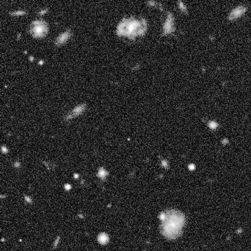
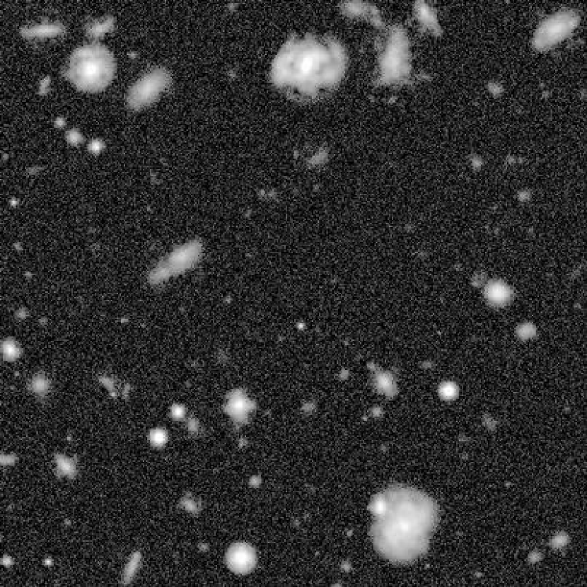
Figure 1: 30$\arcsec\times$ 30$\arcsec$ portions of simulated SNAP $I$-band images, using the PSF shown in figure 2. Left panel: to the depth of the proposed SNAP wide survey. Right panel: to the depth of the Hubble Deep Fields. The SNAP deep survey will be some 2 magnitudes deeper than the latter, but further real data from the ACS on HST are needed to simulate this depth accurately.

2.1 Procedure

The shapelet formalism (Refregier 2003; Refregier & Bacon 2003; summarized in §2.2) has been used to model all the galaxies in the HDFs. Using just a few numbers, this parameterization captures the detailed morphology of the galaxies, including spiral arms, arbitrary radial profiles and irregular substructure. The parameters for each galaxy are stored in a multidimensional parameter space. This is then randomly re-sampled, to simulate new and unique galaxies with realistic properties as compared to those in the original HDFs. A detailed description of the simulation procedure and performance can be found in Massey et al. (2003).

The simulated images are built up with galaxies of all types (spiral, elliptical and irregular) in their observed proportions, with realistic number counts and a size distribution reproducing that in the HDF. Their morphology distribution as a function of magnitude also reproduces that in the HDF. Most importantly, all of these objects possess a precisely known shape, magnitude, size and shear. The amount of shear can be adjusted in shapelet space as an input parameter.

Observational effects including PSF convolution, pixelization, noise and detector throughput are then incorporated in the simulations. In §2.3 we describe the engineering specifications we have used to emulate the performance of the SNAP satellite. In §3 we then attempt to recover the known input shear from these realistic, noisy images using existing (and independent) shear measurement methods.

2.2 Shapelets

Here we briefly describe the idea of shapelets, which is at the core of our image simulation package. More comprehensive details are available in Refregier (2003), Refregier & Bacon (2003), and Massey et al. (2003). Shapelets are an orthonormal basis set of 2D Gauss-Hermite functions. They can be used to model any localized object by building up its image as a series of successive basis functions, each weighted by a “shapelet coefficient”, rather like a Fourier or wavelet transform. Each polar basis state and shapelet coefficient can be identified by two integers: $n\geq 0$ describing the number of radial oscillations, and $m\in\{-n,n\}$ the azimuthal oscillations, or rotational degrees of symmetry. The basis is complete when the series is summed to infinity, but it is truncated in practice at a finite $n_{max}$. This offers image compression because an object is typically well-modelled using only a few shapelet coefficients.

Conveniently, the shapelet coefficients are Gaussian-weighted multipole moments (with the rms width of the Gaussian known as the shapelet scale size $\beta$), as commonly used in various astronomical applications. The $n=2$ states are thus Gaussian-weighted quadrupole moments, the $n=4$ states octopole moments, etc. Shapelet basis functions also happen to be eigenstates of the 2D Quantum Harmonic Oscillator, with $n$ and $m$ corresponding respectively to energy and angular momentum quantum numbers. This analogy suggests a well-developed formalism. For instance, shears and dilations can be represented analytically as $\hat{a}$ or $\hat{a}^{\dagger}$ ladder operators (Refregier 2003); and PSF convolutions as a trivial bra-ket matrix operation (Refregier & Bacon 2003).

Massey et al. (2003) demonstrate how HDF galaxies can be represented as shapelets and then transformed by slight adjustments of their shapelet coefficients into new shapes. This process produces genuinely new but realistic galaxies, as proved by the similar distributions in HDF and simulated data of commonly used diagnostics from SExtractor (Bertin & Arnouts 1996) and galaxy morphology packages (e.g. Conselice, Bershady & Jangren 2000).

2.3 SNAP Simulations

For this work, our image simulations have been tuned to the instrument and specifications of the proposed SNAP mission (paper I; Aldering et al. 2002; Kim et al. 2002; Lampton et al. 2002a, 2002b; Perlmutter et al. 2002). The SNAP strategy includes a wide, 300 square degree survey (with 4$\times$500s exposures reaching a depth of AB 27.7 in R for a point source at $5\sigma$), and a deep, 15 square degree survey (120$\times$4$\times$300s to AB 30.2). For an exponential disc galaxy with FWHM=0.12”, these limits become 26.6 and 28.9 respectively.

The predicted SNAP PSF at the middle of the illuminated region of the focal plane is illustrated in figure 2. Following the analysis of paper I, this was obtained for the current satellite design, using raytracing, aperture diffraction and CCD diffusion. In this paper we also illustrate the decomposition of the SNAP PSF into shapelets. As shown on the top panel of figure 2, our model includes the second diffraction ring and is accurate to nearly one part in 10³. It does not include much of the extended low-level diffraction spikes, which we ignore. Convolution with this residual PSF pattern adds less than 0.7% to the ellipticity of any exponential disc galaxy that passes the size cut into the lensing catalog (see $\S\ref{method}$). Given the further factor of $G^{-1}$ in equation [4], to convert ellipticity into shear, this residual thus has a negligible impact upon shear measurement within the accuracy of the current methods.

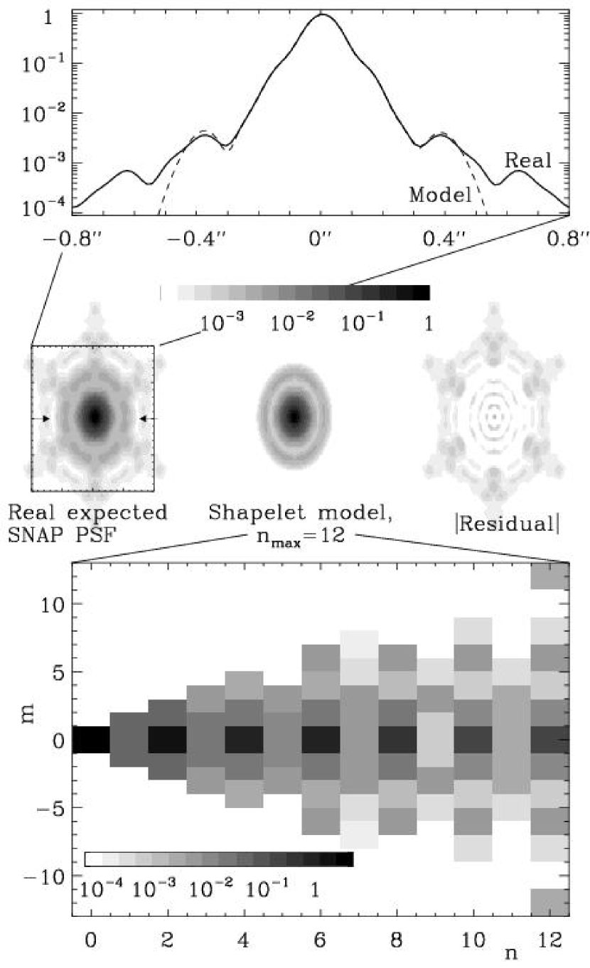
Figure 2: Shapelet decomposition of the proposed SNAP PSF. Top panel: a horizontal slice through the center of the real (solid line) and shapelet-reconstructed (dashed line) PSF. The middle panels shows, in 2-dimensions, the real PSF, its recovery using shapelets and the residual difference between the two, from left to right respectively. Bottom panel: the moduli of the corresponding polar shapelet coefficients with order up to $n_{max}=12$. Note that all intensity scales are logarithmic. The circular ($m=0$) core is modelled to an accuracy of about $10^{-3}$ and the beginnings of six-fold symmetric structure is seen as power in the $m=\pm 6,\pm 12$ shapelet coefficients.

Simulated images used to calibrate the shear measurement method (see §3.2) were first sheared and then convolved with the full SNAP PSF shown in figure 2. For this application, it is essential that the shearing is applied before the smearing, just as occurs in the real universe. Shear measurement methods have been designed to correct for precisely this sequence of events. However, our simulated galaxies were modelled on real HDF objects which had already been naturally convolved with the WFPC2 PSF when the HDF images were taken. Consequently, our simulated objects in §3.2 exhibit smoothing from both a circularised WFPC2 PSF, (plus shearing), plus a SNAP PSF. This double PSF artificially reduces the rms ellipticity of galaxies by approximately $\sim$2% and increases the size of a point source by 22%. One should note that the first PSF convolution occurs, and the galaxy orientations are randomized, all before shearing. This effect therefore corresponds to a small alteration in the intrinsic shape distribution of galaxies but does not bias the shear measurement (see discussion in Massey et al. 2003).

Simulated images used to predict the lensing efficiency as a function of exposure time (see §3.3) were produced differently. For these, we needed to ensure realistic size distributions and number counts in the simulations. The galaxies had no artificial shear added: they just have a scatter of ellipticities due to their own intrinsic shapes. We convolved these galaxies by the PSF difference between the HST and SNAP. This is obtained by deconvolving the WFPC2 PSF from the SNAP PSF model, in shapelet space. Smoothing an object with this smaller kernel is enough to convert it from an observation with HST to one with SNAP, although without inputting shear.

Example simulated images are shown in figure 1 for the wide SNAP survey (left panel) and to the depth of the HDF (right panel). They include a noise model consisting of both photon counting error and a Gaussian background. These compare well with real deep HST images (see Massey et al. 2002). The SNAP deep fields will be about 2 magnitudes deeper than the HDF. However, deeper surveys with the ACS on board HST are awaited to accurately model galaxies at this depth. Figure 3 shows the size-magnitude distribution of the simulated images to both depths (top panels). Again, the simulations reproduce the statistics of the real HDFs (bottom panels).

2.4 Limitations of the Simulations

The SNAP wide survey strategy includes four dithered exposures at each pointing. This will enable the removal of cosmic rays and, if necessary, the simultaneous measurement of instrumental distortions. Because of the high orbit and slow thermal cycle, instrument flexure and the PSF are expected to be very stable (see paper I). It should therefore be possible to map internal distortions and compensate for them even on small scales, using periodic observations of stellar fields. Consequently, neither cosmic rays nor astrometric distortions are added to the simulations.

The SNAP CCD pixels are 0.1$\arcsec$ in size and thus under-sample the PSF. To compensate for this, the dithered exposures will be stacked, as usual for HST images, using the DRIZZLE algorithm (Fruchter & Hook 2002). Alternatively, galaxy shapes may be fitted simultaneously from several exposures. DRIZZLE recovers some resolution, and will be particularly effective for the multiply-imaged SNAP deep survey, but has the side-effect of aliasing the image and correlating the noise in adjacent pixels. We have not yet included this entire pipeline in the simulations, but merely implemented a smaller pixel scale and model background noise that is higher in each pixel (although uncorrelated). Following the example of the Hubble Deep Field final data reduction, we choose 0.04$\arcsec$ pixels. Unfortunately, the detection and shape measurement of very faint galaxies is sensitive to the precise noise properties of an image. Because of these instabilities, our simulated images are only reliable down to approximately $I\simeq 29.5$ (see Massey et al. 2003). This is just below the magnitude cut applied by our shear measurement method at $I=29.1$. A further investigation will include full use of DRIZZLE and more detailed noise models. This will also address the issue of pointing accuracy, and consider the consequences of ‘dead zones’ around the edges of the pixels which house the CCD electronics and are therefore unresponsive to light.

Figure 3: Size vs magnitude as determined by SExtractor with a $S/N$ cutoff at $\nu=1.5$. Top panels are for simulated SNAP $I$ band images of the same size as the Hubble Deep Field. For reference, the bottom panels are of the HDFs themselves using the same SExtractor parameters.

The image simulations are based upon the galaxies in the HDF, which is itself a special region of space selected to contain no large or bright objects. As a result, our simulations do not yet include these either. The source catalog is being expanded as GOODS ACS data becomes publicly available.

The image simulations are currently monochromatic, in the HST $F814W$ (hereafter $I$) filter. Since gravitational lensing is achromatic, shear measurement can be performed in any band: indeed, all tested shear measurement methods so far use only one color at a time. $I$ or $R$ bands are typically chosen for shear measurement because of the increased galaxy number density, advanced detector technology, and small PSF at these wavelengths. Surveys like COMBO17 (Brown et al. 2003), and VIRMOS/Descartes (van Waerbeke et al. 2002) are leading a trend to use additional multicolor photometry to provide photometric redshifts of the source galaxy population. The SNAP surveys will be simultaneously observed in 9 bands: 6 optical colors spanning roughly $B\rightarrow I$, plus $J$, $H^{\prime}$ and $K$ (the near IR filters are twice as large and receive double the total exposure times given in $\S\ref{makesims}$; see paper I). We have not simulated this multicolor data, but it will inevitably raise the S/N of shear estimation for every source galaxy. At a minimum, image coaddition or simultaneous fits to shapes in several colors will increase the effective exposure time. Something more ambitious, like shifting to the rest-frame $R$ or the rotating disc dis-alignment suggested by Blain (2002), might even reduce systematic measurement biases. Further work is needed in cosmic shear methodology to investigate the optimal use of multicolor data. However, it can already be said that our current monochromatic approach will yield a conservative estimate of the lensing sensitivity expected from future analyses.

3 Weak Lensing sensitivity

In this section, we determine the accuracy with which it is possible to recover the input shear from the noisy image simulations. The formalism of shapelets can be used to form an accurate shear measurement (Refregier & Bacon, 2003). However, since the images themselves were created using shapelets, we choose here to be conservative and use a slightly older but independent method developed by Rhodes, Refregier & Groth (2000; RRG).

3.1 Advantages of space

We first discuss the advantages specific to weak lensing measurement that are provided by observations from space. The figure of merit for any lensing survey needs to include more than the étendue, a product of the survey area and the flux gathering power of a telescope (Tyson et al. 2002, Kaiser et al. 2002). It must also account for the finite PSF size, the size-magnitude distribution of background galaxies, and systematics (e.g. due to the atmosphere or telescope optics). Shear sensitivity is raised for a spacecraft over a ground-based telescope for the additional reasons listed below.

• More objects have measurable shapes. Although not as much sky area will be surveyed as by proposed ground based surveys such as MEGACAM (Boulade et al. 2000), VISTA (http://www.vista.ac.uk), or LSST (http://www.lsst.org), the number density of resolved objects is an order of magnitude higher from space (compare figure 5 with Bacon et al. 2001). Such an increase in $S/N$ per unit area will enable the mapping of projected dark matter maps with adequate resolution for a direct comparison to redshift surveys ($\S\ref{2dmap}$) and the generation of a mass-selected cluster catalog (e.g. Weinberg & Kamionkowski 2002, Hoekstra 2002). Quantitative study of high-sigma mass fluctuations is one of the most promising methods to break degeneracies in cosmological parameter estimation, particularly constraining $\Omega_{\rm m}$ (e.g. van Waerbeke & Mellier 1997; Cooray, Hu & Miralda-Escudé 2000; Munshi & Jain 2001; Schneider 2002). Furthermore, studying well-resolved groups and clusters individually, rather than statistically, will lead to a better understanding of astrophysical phenomena such as biasing or the mass-temperature relation (Weinberg et al. 2002; Huterer & White; 2003 Smith et al. 2003).

• The shape of individual galaxies are more precisely measured. The SNAP PSF is small (0.13$\arcsec$ FWHM assuming 4$\mu$m CCD diffusion). It is more isotropic and, importantly, more stable than even the HST PSF (see paper I). This enables shape measurement to be more reliable, or possible at all, for small, distant galaxies. The stable photometry from the 3-day orbit may even permit the use of weak lensing magnification as well as shear information (see e.g. Jain 2002; 2003). Whether directly measured or inferred from shear, this in turn is useful to correct for the effect of lensing on the distance moduli to the SNAP supernovæ (Dalal et al. 2003; Perlmutter et al. 2002).

• Galaxy redshifts are known accurately and to a greater depth. SNAP’s stable 9-band optical and NIR imaging is ideal to produce exquisite photometric redshifts for almost all galaxies at $z\lesssim 3$ detected at 5$\sigma$ in the $I$-band (see $\S\ref{photoz}$). This should be compared to the $\sim$38% completeness of photo-$z$s possible from the ground in the COMBO-17 data with a similar cut and a median redshift of $R\simeq 24$ (Brown et al. 2002). This allows a good estimation of the redshift distribution of source galaxies, the uncertainty in which is a major contribution to the error budget in current lensing surveys. Projected 2D power spectra and maps can be drawn in several redshift slices, using redshift tomography. More ambitiously, cluster catalogs and dark matter maps can be constructed directly in 3D ($\S\ref{3dmap}$), enabling the 3D correlation of mass and light and the tracing of the growth of mass structures.

• Galaxies are farther away. Distant objects, too faint and too small to be seen from the ground, are measurable from space. The evolution of structures can thus be traced from earlier epochs, giving a better handle on cosmological parameters (see paper III). Furthermore, recent numerical simulations (Jing 2002; Hui & Zhang 2002) suggest that intrinsic galaxy alignments impact lensing surveys to a greater depth in redshift than previously assumed. If this is confirmed, intrinsic alignments will mimic and bias cosmic shear signal in all but the deepest surveys, where the galaxies are farther apart in real space. Using 3D positions of galaxies from SNAP photo-$z$s, it will be possible to isolate close galaxy pairs and to measure their alignments, or to optimally down-weight close pairs thus reducing their impact (King & Schneider 2002; Heavens & Heymans 2002).

3.2 Shear measurement method

The advantages of space-based data described above will provide limited gains without an equally precise and robust shape measurement method. The now-standard weak lensing method for ground-based data was introduced by Kaiser, Squires & Broadhurst (1995; KSB). KSB forms shear estimators from quadrupole and octopole moments of an object’s flux. Modern techniques are being developed to incorporate higher order shape moments or Bayesian statistics to raise the sensitivity to shear. These methods include shapelets (Refregier & Bacon, 2003) and others by Bernstein & Jarvis (2001); Bridle et al. (2003); Kaiser (2000). However, since the simulations themselves were created using shapelets, we choose here to be conservative and use the independent method developed by Rhodes, Refregier & Groth (2000; RRG). This is related to KSB, but optimized for use with space-based data. It has already been used extensively on HST images (Rhodes et al. 2001; Refregier et al. 2002) and is therefore appropriate for our current purposes.

Following KSB, RRG measures a galaxy’s two-component ellipticity $\varepsilon_{i}$ from the Gaussian weighted quadrupole moments of its surface brightness $I({\mathbf{\theta}})$,

$$\varepsilon_{i}\equiv\frac{\{J_{11}-J_{22},~{}2J_{12}\}}{J_{11}+J_{22}}$$ (1)

where

$$J_{ij}\equiv\frac{\int d^{2}\theta~{}\theta_{i}~{}\theta_{j}~{}w({\mathbf{\theta}})~{}I({\mathbf{\theta}})}{\int d^{2}\theta~{}w({\mathbf{\theta}})~{}I({\mathbf{\theta}})}~{},$$ (2)

and $w({\mathbf{\theta}})$ is a Gaussian of width adjusted to match the galaxy size. The unweighted PSF moments are measured from a (simulated) starfield and RRG corrects the galaxy ellipticities to first order for PSF smearing. Occasional unphysical ellipticities, $|\varepsilon|>2$, are excluded, along with galaxies fainter than AB 26.5 (for the SNAP wide survey) or AB 29.1 (for the SNAP deep survey) and with sizes

$$R\equiv\sqrt{\frac{1}{2}\left(J_{11}+J_{22}\right)}\leq 1.7\mathrm{pixels}.$$ (3)

Note that $R$ is an rms size measure rather than a FWHM, and that this procedure does indeed select only resolved objects. The locations of these cuts have been chosen to yield reasonably stable results; the effect of moving the size cut is discussed further in section §3.4.

RRG finally provides the shear susceptibility conversion factor, $G$, to generate unbiased shear estimators $\hat{\gamma}_{i}$ for an ensemble of objects, given by

$$\hat{\gamma}_{i}=\frac{\langle\varepsilon_{i}\rangle}{G}~{},$$ (4)

where $G$ depends upon the fourth order moments $J_{ijkl}$ of a galaxy population, defined similarly to equation [2]. In our simulated SNAP images, $G$ is of order 1.6.

Figure 4: The applied shear $\gamma_{in}$ in the shapelet simulated images vs its recovery $\gamma_{out}$ using an independent measurement method (Rhodes, Refregier & Groth 2000). The image used is one $7.5$ arcmin² realization of the SNAP deep survey shown in figure 1. The recovery is linear, but the slope of the fitted line (dotted) is flatter than that expected (dashed line).

This shear measurement method and the simulations are tested in figure 4. An artificial shear is applied uniformly upon all objects in a $7.5$ arcmin² simulated image, in the $\gamma_{2}=0$ and $\gamma_{1}=0$ directions, before convolution with the SNAP PSF. Using RRG, we correct for the PSF smearing and recover the input shear. As can be seen in figure 4, the recovery is linear, but the slope (see dotted line) is underestimated (dashed line). This inconsistency probably has two origins: inaccuracy of the image simulations and instabilities in the shear measurement method. The latter may be removed with future techniques. For the purposes of this paper, we follow the procedure adopted by Bacon et al. (2001), where a similar bias was observed in the KSB method. We apply a linear correction factor to the measured shears and to their errors. This factor is $(0.79\pm 0.03)^{-1}$ at the depth of the HDF, and $(0.87\pm 0.04)^{-1}$ for the SNAP wide survey.

Even after this correction, there remains a small difference in the rms scatter of galaxy ellipticities between the simulations and real Groth strip data (Rhodes, Refregier & Groth 2001). As shown in Massey et al. (2003), this discrepancy is not detected with the standard shape measures of SExtractor (Bertin & Arnouts 1996), however RRG proves to be a more sensitive test. Perhaps because of the precise properties of the background noise, or perhaps because the wings of simulated objects are truncated beyond the SExtractor isophotal cutoffs, $\sigma_{e}$ is observed by RRG to be lower in the simulated images by another factor of $\sim 0.8$. Work is in progress to establish the origin of this effect. For the purposes of this paper, we simply increase the error bars by this amount.

3.3 Shear sensitivity of SNAP

Now that the image simulation and analysis pipeline is in place, we can measure SNAP’s sensitivity to shear. Trade-off studies are under way for several alternative telescope designs, including the level of CCD charge diffusion, the pixel size, the effect of DRIZZLEing, and the coefficient of thermal expansion in the secondary struts, which may be the main cause of temporal variation in the PSF (see paper I). Here we present the results of a study which uses the baseline design specifications and time-averaged PSF of the SNAP satellite. In this study the PSF used is the residual between the HST and SNAP PSFs (see §2.3), in order to keep the size distribution of galaxies realistic for SNAP images.

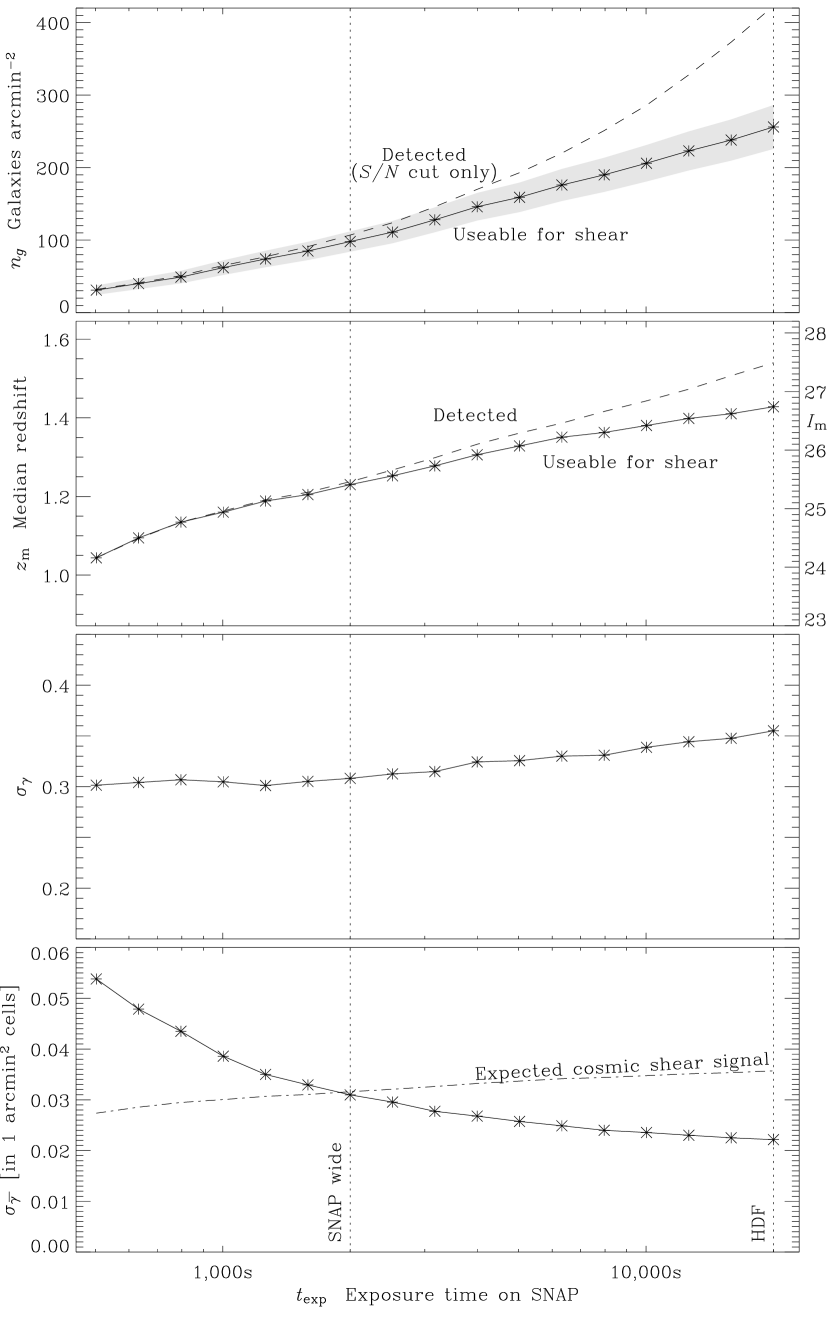
Figure 5: Shear sensitivity as a function of SNAP exposure time $t_{\rm exp}$. Top panel: the surface number density of all galaxies ($n_{g,{\rm tot}}$) detected by SExtractor and of the subset ($n_{g}$) of these useable for weak lensing, i.e. having survived further cuts in size and ellipticity by RRG (see text). Second panel: the median $I$ band magnitude, $I_{\rm m}$, in the two subsets of the galaxy catalog, which has been interpreted as median redshift, $z_{\rm m}$, using equation [8]. Third panel: the rms error $\sigma_{\gamma}=\langle|\gamma|^{2}\rangle^{1/2}$ per galaxy for measuring the shear $\gamma$, after PSF correction and shear calibration. Bottom panel: the rms error $\sigma_{\overline{\gamma}}$ for measuring the mean shear $\overline{\gamma}$ in 1 arcmin² bins. The dot-dashed line shows an estimate of the expected rms shear in a $\Lambda$CDM universe.

The top panel of figure 5 shows the surface number density $n_{g}$ of galaxies in a survey of a given exposure time $t_{\rm exp}$ on SNAP. The exposure times reflect a $\sim 5\times$ overall improvement in instrument throughput and detector efficiency over WFPC2 on HST (Lampton et al. 2002). The dashed line shows the number density $n_{g,{\rm tot}}$ of all the galaxies detected by SExtractor, after a $S/N$ cut which is equivalent to $I<29.1$ at the depth of the HDF. As discussed in $\S\ref{method}$, galaxies which are too faint, too small, or too elliptical are excluded from weak shear catalogs. The solid line shows the number density $n_{g}$ of galaxies which are useable for weak lensing following the magnitude, size and ellipticity cuts. The error bars reflect the uncertainty in measuring number counts at low $S/N$ and an estimated sample variance between the HDF-N and HDF-S.

An important cut in the weak lensing analysis is the size cut, which reduces the detected galaxy sample by about 30% at the depth of the HDF. This fraction is a strong function of PSF size, and is thus much larger for ground based imaging. As can be inferred from the top panel of figure 5, the SNAP wide survey ($n_{g}\simeq 100$ galaxies arcmin^-2) will thus provide a dramatic improvement over current ground-based surveys ($n_{g}\sim 25$ galaxies arcmin^-2 are used by most groups; see e.g. Bacon et al. 2002). The effect of moving the size cut is discussed further in section §3.4.

The second panel of figure 5 shows the median magnitude, $I_{\rm m}$, of the galaxy catalog before and after cuts in size and ellipticity by the weak lensing analysis software. This has been converted to a median redshift, $z_{\rm m}$, using equation [8]. For the purposes of this plot, we assume that this relationship is still valid even after the size cut.

The third panel of figure 5 shows the rms error $\sigma_{\gamma}=\langle|\gamma|^{2}\rangle^{1/2}$ per galaxy for measuring the shear, after the PSF correction and shear calibration. The slightly increasing error at longer $t_{\rm exp}$ reflects the decreasing size of fainter galaxies, and correspondingly less resolved information content available about their shapes. To map the shear, the noise can be reduced by binning the galaxies into cells. The rms noise of the shear $\overline{\gamma}$ averaged in a cell of solid angle $A=1$ arcmin² is given by

$$\sigma_{\overline{\gamma}}\simeq\frac{\sigma_{\gamma}}{\sqrt{n_{g}A}},$$ (5)

and is plotted in the bottom panel of figure 5. The wide and deep SNAP surveys will thus afford a $1\sigma$ sensitivity for the shear of $\simeq 3.0$% and better than $2.2$% on this scale, respectively. As a comparison, the rms shear expected from lensing on this scale in a $\Lambda$CDM model is approximately 3% (assuming $\Omega_{\rm m}$=0.3, $\Omega_{\Lambda}$=0.7, $\sigma_{8}$=0.9, $\Gamma$=0.21). This signal increases with survey depth because the total lensing along a line of sight is cumulative. The wide SNAP survey will thus be ideal to map the mass fluctuations on scales of 1 arcmin², with an average $S/N$ of unity in each cell. The recovery of simulated mass maps will be discussed in $\S\ref{maps}$.

Note that the shear sensitivities presented here are conservative estimates, particularly for the deep SNAP survey. The image simulations extend so far only to the depth of the HDF. Future shear measurement methodology will also be more accurate and stable on any individual, resolved galaxy than the RRG method used in this paper. Higher order shape statistics (e.g. shapelets) will be used, as will simultaneous measurements in multiple colors and pre-selection of early-type galaxy morphologies.

3.4 Effect of size cut and pixel scale

Small, faint and highly elliptical objects are excluded from the final galaxy catalog in the RRG shear measurement method. Of all these cuts, it is the size cut that excludes the most objects. In an image at the depth of the HDF, about 30% of detected galaxies are smaller than our adopted size cut at $R=1.7$ pixels. The exact position of this cut has been determined empirically to produce stable results, from experience with both HST data and our simulated images. The quantitative effects of moving the size cut are demonstrated in figure 6.

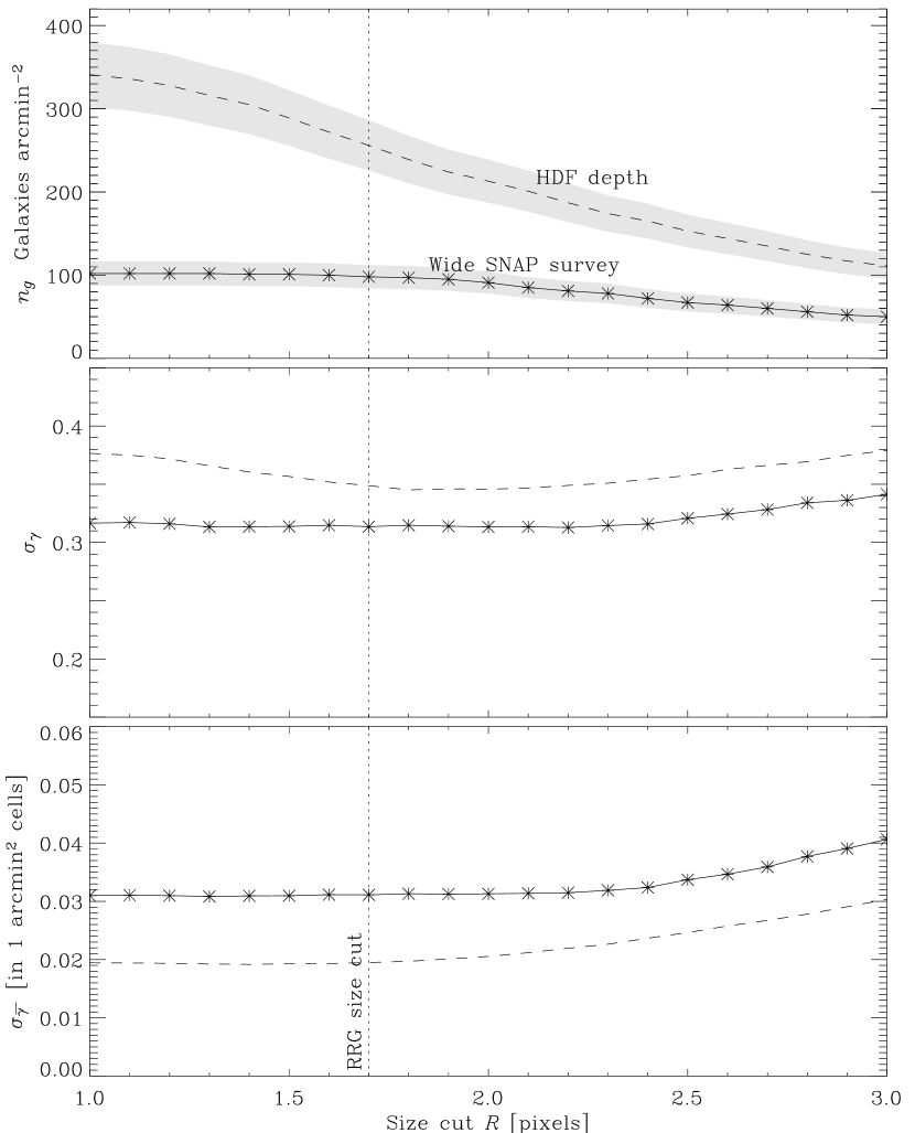
Figure 6: Shear sensitivity as a function of size cut $R$ in the RRG shape measurement method for the wide SNAP survey (solid line) and at the depth of the HDF (dashed line). The vertical dotted line shows the fiducial value adopted elsewhere in our analysis. Top panel: the surface number density of galaxies useable for weak lensing. Middle panel: the rms error $\sigma_{\gamma}=\langle|\gamma|^{2}\rangle^{1/2}$ per galaxy for measuring the shear $\gamma$, after PSF correction and shear calibration. Bottom panel: the rms error $\sigma_{\overline{\gamma}}$ for measuring the mean shear $\overline{\gamma}$ in 1 arcmin² bins.

If the cut is moved to a larger size, fewer objects are allowed into the final galaxy catalog, and the shear field is sampled in fewer locations. Consequently, both dark matter maps and cosmic shear statistics become more noisy. If smaller galaxies are included in the catalog, the shear field is indeed better sampled, but the shape measurement error is worse on these galaxies. The bottom panel of figure 6 shows that moving the size cut to smaller objects has no net change in the precision of shear recovery: adding noisy shear estimators to the catalog neither improves nor worsens the measurement. A size cut at $R=1.7$ pixels is optimal at the depth of the HDF and in the observing conditions modelled by our image simulations. To simplify comparisons of galaxy number density, the same cut has been applied to data at the depth of the SNAP wide survey. A different cut could have been adopted, producing fewer galaxies but each with more accurate shear estimators: the crucial figure $\sigma_{\hat{\gamma}}$ would not change. (This is especially true in the SNAP wide survey because of the relative dearth of small galaxies).

As described in section 2.4, we have assumed that an effective image resolution of 0.04” can be recovered for SNAP data by taking multiple, dithered exposures, and either stacking them with the DRIZZLE algorithm or by fitting each galaxy’s shape simultaneously in them all. The increase in image resolution from these techniques is vital for cosmic shear measurements. The number density of useable galaxies increases dramatically, and the measurement of their shapes is improved. Were it not possible to apply DRIZZLE or to recover this resolution, the large pixel scale currently proposed for SNAP would seriously impair shear measurement. A size cut at $R=0.12\arcsec$ ($=3$ pixels in figure 6) would roughly halve the number density of useable sources and correspondingly reduce the sensitivity to gravitational lensing.

4 Photometric Redshift Accuracy

Gravitational lensing is achromatic, so shear measurement may be performed in any color. As discussed in $\S\ref{simlims}$, current techniques measure galaxy shapes in only one band at a time (usually $R$ or $I$ are chosen for their steeper slope of number counts). However, gravitational lensing is also a purely geometrical effect, and measurements are aided greatly by accurately knowing the distances to sources. The latest surveys, and future high-precision measurements will therefore require multiple colors for photometric redshift (photo-$z$) estimation. Reliable photo-$z$s will not only remove current errors due to uncertainty in the redshift distribution of background sources, but even make possible an entirely 3D mass reconstruction, as demonstrated in $\S\ref{3dmap}$, Taylor (2003a), Hu & Keeton (2002), Bacon & Taylor (2002) and Jain & Taylor (2003).

SNAP’s thermally stable, 3-day long orbit is specifically designed for excellent photometry on supernovæ. Combining all 9 broad-band filters (6 optical, 3 NIR) will also provide an unprecedented level of photo-$z$ accuracy, for all morphological types of galaxies over a large range of redshifts. In this section, we simulate SNAP photometric data in order to determine this precision.

We have used the hyperz code (Bolzonella, Miralles & Pelló 2000) to generate the observed magnitudes of a realistic catalog of galaxies following Lilly et al. (1995),

$$\frac{{\mathrm{d}}N}{{\mathrm{d}}I}(I)\simeq 10^{0.35\times I}~{},$$ (6)

where $I$ is the $I$-band magnitude. The galaxies were assigned a distribution of Spectral Energy Distribution (SED) types similar to that in real data and containing ellipticals, spirals and starburst galaxies. Redshifts were assigned at random, and independently of spectral type, according to Koo et al. (1996) as verified by the DEEP collaboration (1999),

$$\frac{{\mathrm{d}}N}{{\mathrm{d}}z}(z)\simeq z^{2}e^{-\left(z/z_{m}\right)^{2}}~{},$$ (7)

where

$$z_{m}=0.722+0.149(I-22.0)$$ (8)

(Lanzetta, Yahil & Fernandez-Soto 1996). SNAP colors were then inferred by integrating the SED across filter profiles, adding an amount of noise corresponding to the exposure time and instrument throughput.

Hyperz was then used again, to estimate redshifts for the simulated catalog as if it were real data. Unlike the image simulations in $\S\ref{sims}$, this approach can already be taken to the depth of both the wide and the deep SNAP surveys by extrapolating functional forms for the luminosity and redshift distributions (eqs. [6] & [7]). Magnitude cuts were applied at AB 26.5 (wide) or AB 29.1 (deep) in $R$. Similar magnitude cuts were made in each filter, chosen at the $10\sigma$ detection level of an exponential disc galaxy with FWHM=0.12$\arcsec$ (Kim et al. 2002). Past experience with lensing data (see $\S\ref{method}$, Bacon et al. 2000) confirms that this is reasonable $S/N$ limit. Note however that the size and ellipticity cuts implemented for the simulated images in $\S\ref{method}$ were not included at this stage.

Figure 7: Recovery of redshifts of a realistic population of galaxies using hyperz with the SNAP filter set. Top-left panel: the wide survey, using all 9 colors. Top-right panel: the deep survey using all 9 colors. Bottom row: the same, but with only the 6 optical colors, as if the near IR HgCdTe data were not available.

Figure 7 shows the precision of photometric redshifts in both the wide and deep SNAP surveys. All galaxy morphological types are included in this analysis. Clearly demonstrated is the need for the near IR HgCdTe detectors, a component of the satellite where a spacecraft has a clear advantage over the ground. Figure 8 shows the accuracy of the photo-$z$s as a function of source (photometric) redshift. Here, $\Delta z_{\rm photo}(z)$ is the rms of the core Gaussian in a double-Gaussian fit to horizontal slices through the distributions in figure 7.

Figure 8: $\Delta z_{\rm photo}$, the rms scatter on photometric error estimation, as a function of increasing source redshift, $z$. Top panel: results for the SNAP deep survey. Bottom panel: results for the SNAP wide survey. In both cases, the solid line shows photometric redshift errors using observations in all 9 SNAP optical and near IR colors. The dashed lines show errors if the near IR HgCdTe data were unavailable.

To estimate the accuracy of 3D mass reconstructions (§5.2), we now concentrate on objects closer than $z=1$. According to equations [6] and [7], these make up $\sim 38$% of all galaxies detected in $R$ for the wide SNAP survey, and $\sim 35$% for the deep. For the lensing analysis ($\S$3.2), we have to reject some fraction of galaxies because they were too small & not resolved. Here, we assume that the same percentage of rejection applies to the $z<1$ sub-sample of galaxies. This will yield a conservative estimate of the number of objects remaining in the real SNAP survey because objects closer than z=1 are likely to have a larger median size than the entire sample. Removing this fraction from the number density of galaxies shown in figure 5 leaves $40\pm 5$ useful galaxies per arcmin² in the SNAP wide survey to $z=1$, and more than 90arcmin^-2 in the SNAP deep survey. For these galaxies only, $\Delta z_{deep}=$0.034 and $\Delta z_{wide}=$0.38 using all nine SNAP colors.

5 Dark Matter Mapping

In this section, we describe the prospects of a space-based weak lensing survey for mapping the 2D and 3D distribution of dark matter. Because of the high number density of background galaxies resolved from space, this is one application where a mission like SNAP will fare particularly better than surveys from the ground.

5.1 2D Maps

To simulate observational data, we begin with shear maps created by raytracing through N-body simulations from Jain, Seljak & White (2000). We then add noise to these idealized data, corresponding to the predicted levels for SNAP or observing conditions at the currently most successful ground-based facilities. In each case, we then attempt to recover the input projected mass distribution by inverting the map of the shear into a map of the convergence $\kappa$. Convergence is proportional to the projected mass along the line of sight, by a factor depending on the geometrical distances between the observer, source and lensed galaxies (see e.g. Bartelmann & Schneider, 2001).

Figures 10 and 10 show how the projected mass can be mapped from space and from the ground. The color scale shows the convergence $\kappa$. The top panel of figure 10 shows a (noise-free) simulated convergence map from the ray tracing simulations of Jain, Seljak & White (2000) for an SCDM model. Underneath it is a version smoothed by a Gaussian kernel with an rms of $1\arcmin$ for comparison to the simulated recovery from observational data in figure 10.

Figure 10 shows similarly smoothed mass maps that would be possible using (from top to bottom) a ground-based survey, the SNAP wide survey and the SNAP deep survey. These were produced by adding to $\kappa$, before smoothing, Gaussian random noise to each 1 arcmin² cell with an rms of $\sigma_{\overline{\gamma}}$ given by equation [5]. Overlaid contours show mass concentrations detected at the 3$\sigma$, 4$\sigma$ and 5$\sigma$ levels. For ground based observations, we set $\sigma_{\gamma}=0.39$, and used $n_{g}=25$ arcmin^-2, as is available for ground-based surveys (e.g. Bacon et al. 2002). For the SNAP wide and deep survey, the surface density of useable galaxies was taken to be $n_{g}=105$ arcmin^-2 and 259 arcmin^-2, and the rms shear noise per galaxy was taken to be $\sigma_{\gamma}=$0.31 and 0.36, respectively, as derived from figure 5. The galaxies are assumed to all have a redshift of $z$=1, which is a good approximation as long as the median redshift is approximately that value. As noted above, the surface density and median redshift will actually be higher for the SNAP deep survey, because only exposure times corresponding to that of the HDF were simulated.

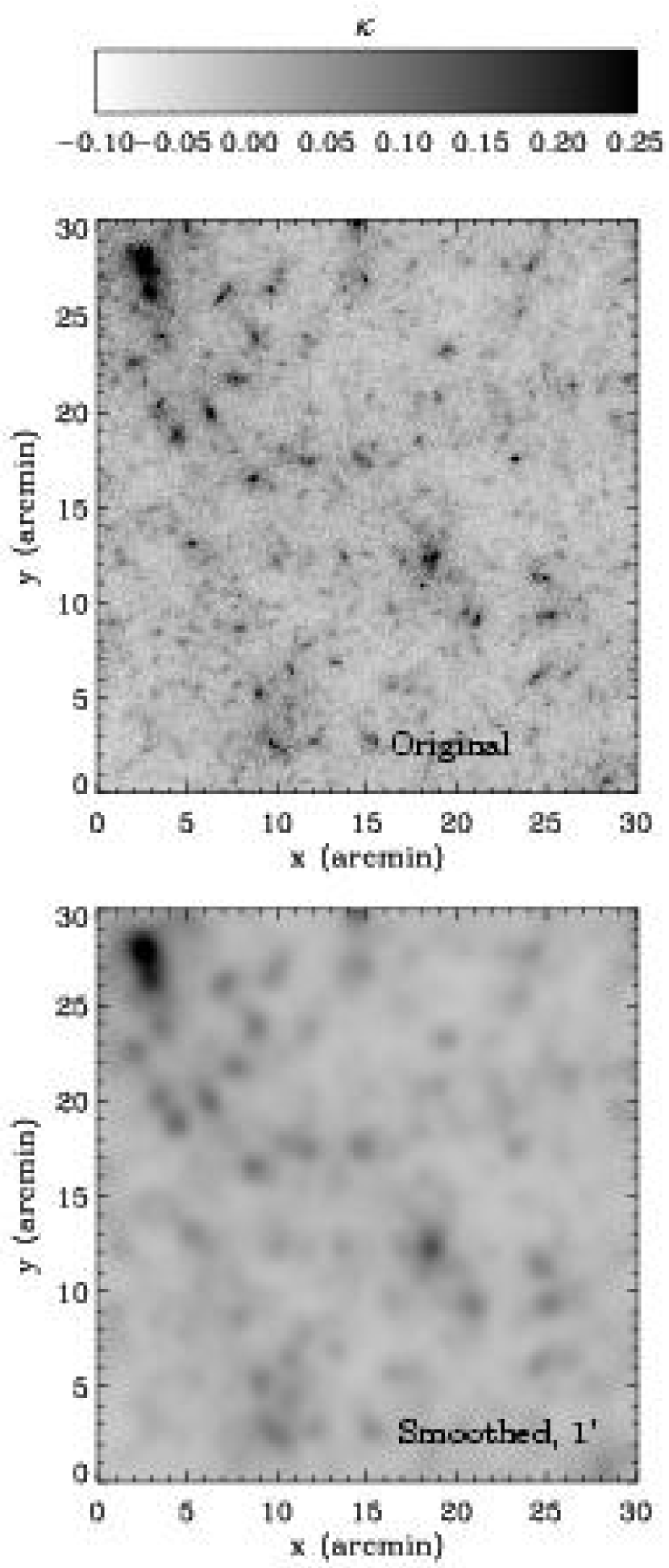
Figure 9: Left column. 2-dimensional convergence maps projected along a line of sight. The convergence $\kappa$ is proportional to the total matter density along the line of sight, and can be deduced from the shear field. Top panel: simulated (noise-free) convergence map derived by ray-tracing through an SCDM N-body simulations of large-scale structure from Jain, Seljak & White (2000). The region shown is 30$\arcmin\times$30$\arcmin$ and the sources are assumed to lie at $z=1$. Bottom panel: same map but smoothed using a Gaussian kernel with a FWHM of 1$\arcmin$.

Figure 10: Right column. Reconstructions of the convergence map in figure 10 which may be feasible from weak lensing surveys on the ground and from space. Overlaid contours show 3$\sigma$, 4$\sigma$ and 5$\sigma$ detection limits. Top panel: convergence $\kappa$ with noise added corresponding to ground-based observations (i.e. $n_{g}=25$ arcmin^-2 and $\sigma_{\gamma}=0.39$; Bacon et al. 2002). Middle panel: convergence map with the expected noise properties of the wide SNAP survey (i.e. $n_{g}=105$ arcmin^-2 and $\sigma_{\gamma}=0.31$). Bottom panel: with the expected noise level of the deep SNAP survey (i.e. $n_{g}=259$ arcmin^-2 and $\sigma_{\gamma}=0.36$).

From the ground,only for the strongest features (i.e. the most massive clusters) can a 3$\sigma$ detection be obtained. From space, the very high density of resolved background galaxies allows the recovery of uniquely detailed maps, including some of the filamentary structure and individual mass overdensities down to the scale of galaxy groups and clusters. Thus, SNAP offers the potential of mapping dark matter over very large fields of view, with a precision well beyond that achievable with ground-based facilities.

The masses and locations of individual clusters can be extracted from such maps using, for example, the $M_{\mathrm{a}p}$ statistic (Schneider 1996, 2002), which has been applied successfully to find mass peaks in several surveys (e.g. Hoekstra et al. 2002a; Erben et al. 2000) and our own work; or the inversion method of Kaiser & Squires (1993; KS) which was used by Miyazaki et al. (2002). Marshall, Hobson & Slosar (2003) demonstrate the effectiveness of maximum entropy techniques to identify structures in KS lensing maps, using criteria set by Bayesian evidence. White et al. (2002) argue that using any detection method, a complete mass-selected cluster catalogue from 2D lensing data would require a high rate of false-positive detections, since the prior probability is for them to be anywhere throughout a given survey. This has been avoided in practice by secondary cross-checks of the lensing data with spectroscopy, deep $x$-ray temperature or SZ observations. Indeed, two previously unknown clusters have already been found in weak lensing maps and spectroscopically confirmed by Wittman et al. (2001, 2003). However, this confusion does make it harder to resolve the debate on the possible existence of baryon-poor “dark clusters” (e.g. Dahle et al. 2003). These are a speculative population of clusters which would be physically different to and absent from the catalogues of optically or $x$-ray selected clusters. Remaining dark-lens candidates (Erben et al. 2000; Umetsu & Futamase 2000; Miralles et al. 2002) have currently been eliminated as chance alignments of background galaxies (or possibly associations with nearby ordinary clusters Gray et al. 2001; Erben et al. 2003). If others could be found in high S/N weak lensing maps, they would present a challenge to current models of structure formation, and need to be accounted for in estimates of $\Omega_{\rm m}$; but they would be unique laboratories to decipher the nature of dark matter.

5.2 3D Maps

The growth of mass structures can be followed in a rudimentary way via photometric redshifts, by making 2D mass maps or power spectra with source galaxies in different redshift slices (see e.g. Bartelmann & Schneider 2000 §4). This technique is useful for a global statistical analysis of a survey in order to constrain cosmological parameters. It is used as such in paper III, to predict possible constraints with SNAP. Tomographic measurements of shear have also led to estimates of mass and radial position of clusters (Wittman et al. 2001, 2003). After this analysis, spectroscopic redshifts were needed to constrain the mass further by fixing the precise radial position of clusters.

An alternative approach, in which one naturally reclaims the radial mass information as well as the transverse density, has been developed by Taylor (2003a) and Hu & Keeton (2002). In this method, the shear pattern on an image is treated as a fully 3D field, by including from the outset the redshift of galaxy shear estimators as well as their 2D position on the sky. Taylor (2003a) shows that there is a simple inversion that relates this 3D distortion field to the underlying 3D gravitational potential.

Using this technique, we now demonstrate the capabilities of SNAP for reconstructing the 3D mass distribution and locating clusters. We apply the simulations of Bacon & Taylor (2003) to the telescope and survey parameters deduced in paper I, §2 and §3 then attempt to recover the gravitational potential of two $M=10^{14}M_{\odot}$ NFW clusters at redshifts of 0.25 and 0.4 and separated by 0.2 degrees on the sky (see Bacon & Taylor, figures 4 & 5). Note that this is specifically a search for clusters, which induce a significant shear signal at one location, rather that integrating the impact of many small objects and filamentary structures in a statistical basis over an entire shear field. Our relatively simple input model is therefore appropriate for our current purposes: it is a common occurrence that, for a line of sight with large shear, a single cluster along a line of sight is responsible for the signal.

First, we calculate the corresponding lensing potential for this field (using the prescription of Bacon & Taylor, equations 9-12; c.f. Kaiser & Squires 1993). As the lensing potential field $\phi$ is an integral of the shear field, we are able to reconstruct $\phi$ with more accuracy than the gravitational potential $\Phi$, which is a function of the second derivative of $\phi$; nevertheless $\phi$ itself contains valuable 3D information. This is discussed in full in Bacon & Taylor (2003). We have used the expected number density of useable galaxies closer than $z=1$ to be a conservative $n_{g}(z<1)=90$ per arcmin², combining results from figure 5 and $\S\ref{photoz}$. In this nearby regime we can approximate $\frac{dn}{dz}\propto z^{2}$. We have taken into account the shot noise arising from intrinsic galaxy ellipticities, using an error on shear estimators for galaxies of $\sigma_{\gamma}=0.36$. We have also included an error on our photometric redshifts of $\Delta z_{\rm photo}=0.034$ throughout $0<z<1$, from $\S\ref{photoz}$.

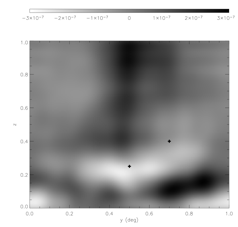
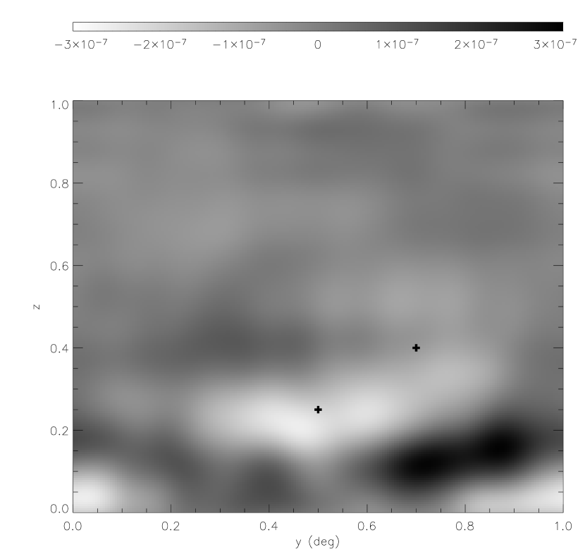
Figure 11: Top panel: reconstructed lensing potential from a finite number of $z<1$ galaxies with realistic ellipticities; $n_{g}=90$ arcmin^-2, $\sigma_{\gamma}=0.36$, as expected for the SNAP deep survey. The $x$-axis represents angle in degrees; the $y$-axis represents redshift. The two crosses mark the positions of the input $M=10^{14}M_{\odot}$ NFW clusters. Bottom panel: difference between input and recovered lensing potential fields.

Figure 11 shows the reconstruction of the lensing potential out to $z=1$ available with the SNAP deep survey. The units of the lensing potential here are radians², having chosen the differential in $\kappa=0.5\partial^{2}\phi$ to be taken in units of radians. In this simulation, we see that the lower redshift cluster is very pronounced in the lensing potential, with S/N per pixel of 5.4 at z=1. The lensing potential due to the higher redshift cluster is also clearly visible, with S/N per pixel of 3.0.

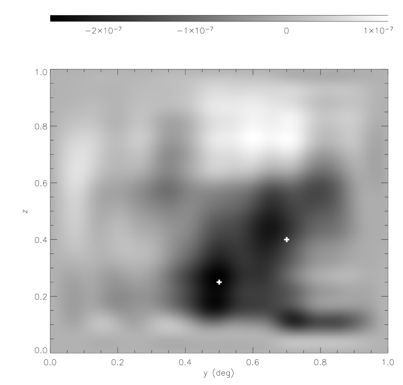
Figure 12: Reconstructed gravitational potential using galaxy properties of the SNAP deep survey, as in figure 11. The $x$-axis represents angle in degrees; the $y$-axis represents redshift. The two input clusters are clearly seen as the two darkest regions near the center of the image, marked with a cross.

Figure 12 shows a reconstruction of the 3D gravitational potential, using Taylor’s inversion and Wiener filtering (Bacon & Taylor equations 8, 40). Even with a simulated mass of only $10^{14}M_{\odot}$, the lower redshift cluster is very pronounced, and the higher redshift cluster is also detectable at the 4.4$\sigma$ level. Extra noise peaks in figure 12 demonstrate that the extremely low end of cluster catalogues will be subject to high false detection rates. However, this reconstruction affords measurement of masses of matter concentrations to an accuracy of $\Delta M\simeq 1.1\times 10^{13}M_{\odot}$ at $z\simeq 0.25$ or $\Delta M\simeq 4.8\times 10^{13}M_{\odot}$ at $z\simeq 0.5$ via $\chi^{2}$ fitting (c.f. Wittman et al. 2001, 2003). We can also estimate radial position of mass concentrations from the simulated lensing data with accuracy $\Delta z\simeq 0.05$ for clusters of mass $M=10^{14}M_{\odot}$ at $z<0.5$ (c.f. Bacon & Taylor 2003). The mass concentrations are observed at $z=0.25$ and 0.4 as expected with peak S/N of 2.8 and 3.3 respectively (N.B. this is S/N per pixel; the overall detection significance of the cluster is as quoted above). Of course, the sensitivity of this technique drops for clusters at greater distances, as their induced lensing potential grows less within the observed redshift window (i.e. $z<1$). In an alternative régime of interest, mass fluctuations $\delta\sim 1$ are measurable on degree scales (c.f. Hu & Keeton 2002).

Equivalent simulations can be carried out for ground-based experiments, providing more limited prospects. The key difference that makes a space-based experiment superior over a ground-based experiment in this regard is the reduced error on shear estimates for galaxies, particularly for galaxies at $z>0.5$, due to improved resolution and small PSF. From the ground, studies of the 3-D $\phi$ field are restricted to measuring the mass of a cluster along the line of sight at the $\Delta M\simeq 2\times 10^{13}M_{\odot}$ level at $z=0.25$, with a $1.3\sigma$ measurement of a mass of $10^{14}M_{\odot}$ at $z=0.5$ along the line of sight of a foreground $z=0.25$ cluster. Reconstruction of $\Phi$ in 3D is possible on 5$\arcmin$ scales only out to a redshift of $z\simeq 0.5$ (see Bacon & Taylor 2003). Application of the full 3D inversion technique to real ground-based data is currently being carried out, and even measurements of one cluster behind another cluster are possible (see review by Taylor 2003a).

SNAP’s ability to measure the 3D gravitational potential in this fashion is of great importance. One can determine the mass and density profile of several matter concentrations along a line of sight, avoiding the ambiguity of surface-density lensing or projection effects, and obtaining accurate measurements of the mass of matter clumps in 3D. One can directly compare the visible matter distribution with the underlying mass distribution to obtain important information regarding biasing and galaxy formation as a function of redshift. One can also examine the number of objects exceeding a certain mass threshold as a function of redshift (see e.g. Viana & Liddle 1996), or reconstruct the 3D power spectrum directly (see Taylor 2003a) in order to obtain constraints on cosmological parameters or to test the gravitational instability paradigm which is thought to govern structure formation.

6 Conclusions

We have shown how a space-based wide field imager like SNAP is ideally suited for studies of weak gravitational lensing. The aspects of this satellite’s design relevant for weak lensing, and the baseline survey strategy, were presented in paper I. A shapelet-based method for creating simulated space-based images (Massey et al. 2003, Refregier 2003) has been used to predict SNAP’s sensitivity to shear, taking explicitly into account its instrumental throughput, limitations and sensitivity.

In this paper, we have considered the baseline SNAP design for our predictions. As explained in paper I, this design is almost optimal because many requirements to find supernovæ are the same as those to measure weak lensing (stable imaging, small PSF, excellent multicolor photometry).

The increased image resolution available from space makes possible the construction of high resolution projected dark matter maps with an rms shear sensitivity of $\sim$2.5% in every 1$\arcmin$ cell for the 300 square degrees wide SNAP survey and better than 1.8% for the SNAP deep survey (c.f. expected mean signal in a $\Lambda$CDM universe is approximately 3%). Since lensing is sensitive to mass regardless of its nature and state, these maps will be unique tools for both astrophysics and cosmological parameter estimation. Statistical properties of the dark matter distribution will be precisely measured at several cosmological epochs and constraints on $\Omega_{\rm m}$, $\sigma_{8}$ and $w$ are discussed in paper III.

SNAP’s simultaneous 9-band observations also open up new opportunities for 3-dimensional mapping via photometric redshift estimation (Taylor 2003a, Hu & Keeton 2002, Bacon & Taylor 2002). SNAP’s photometry allows an excellent resolution of $\Delta z=0.034$ in redshift. Here we have shown that SNAP will measure mass concentrations in full 3D with a 1$\sigma$ sensitivity of approximately $1\times 10^{13}M_{\odot}$ at $z\simeq 0.25$ and $\simeq 5\times 10^{13}M_{\odot}$ at $z\simeq 0.5$. In this fashion it will be possible to directly trace the non-linear growth of mass structures, testing with high precision the gravitational instability theory.

Space-based wide-field imaging can be combined with weak gravitational lensing to produce 2D and 3D mass-selected cluster catalogs down to the scale of galaxy groups. Mass and light in the local universe can be mapped out with exquisite precision, thus offering exciting prospects for both astrophysics and cosmology.

References

- (1) Aldering, G. et al. 2002 Proc. SPIE 4835: 21
- (2) Bacon, D. & Taylor, A., 2003, MNRAS in press
- (3) Bacon, D., Massey, R., Ellis, R. & Refregier, A., 2002 MNRAS in press, astro-ph/0203134
- (4) Bacon, D., Refregier, A., Clowe, D. & Ellis, R., 2001, MNRAS, 325, 1065
- (5) Bartelmann, M. & Schneider, P., 2001, Physics Reports, 340, 291
- (6) Bernardeau, F., van Waerbecke, L. & Mellier, Y., 1997, A&A, 322,1
- (7) Bernardeau, F., van Waerbecke, L. & Mellier, Y., 2002, A&A, 389,28
- (8) Bertin, E., & Arnouts, S., 1996, A&AS, 117, 393
- (9) Blain, A., 2002, ApJ, 570, L51
- (10) Bolzonella, M., Miralles, J.-M. & Pelló, R., 2000, A&A, 363, 476
-
(11)
Boulade, O. et al. , 2000, Procs. SPIE Astronomical
Telescopes and Instrumentation 2000, Munich, 2000; Megacam home page
http://www-dapnia.cea.fr/Phys/Sap/ Activites/Projets/Megacam/page.shtml - (12) Brown et al. , 2002, MNRAS submitted, astro-ph/0210213
- (13) Bridle et al. , 2003, in preparation
- (14) Clowe, D., Trentham, N. & Tonry, J., 2001, , A&A, 369, 16
- (15) Conselice, C., Bershady, M. & Jangren, A., 2000, ApJ, 529, 886
- (16) Cooray, A., Hu, W. & Miralda-Escudé, J., 2000, ApJ, 535L, 9
- (17) Dahle, H., et al. , 2002, ApJ, 139, 313
- (18) Dahle, H., Pedersen, K., Lilje, P., Maddox, S. & Kaiser,N., 2003, ApJ, 591, 662
- (19) DEEP collaboration, 1999, private communication
- (20) Dalal, N., Holz, D., Chen, X. & Frieman, J., 2003, ApJ, 585, L11
- (21) Erben, T., van Waerbeke, L., Mellier, Y., Schneider, P., Cuillandre, J.-C., Castander, J. & Dantel-Fort, M., 2000, A&A, 355, 23
- (22) Fruchter, A. & Hook, R., 2002, PASP, 114, 144
- (23) Gerhard 1993, MNRAS, 265, 213
- (24) Gray, M., Ellis, R., Lewis, J., McMahon, R. & Firth, A., 2001, MNRAS, 333, 544
- (25) Heavens, A., Refregier, A. & Heymans, C., 2000, MNRAS, 319, 649
- (26) Heavens, A. & Heymans, C., 2002, MNRAS submitted, astro-ph/
- (27) Hoekstra, H., van Waerbeke, L.,Gladders, M., Mellier, Y. & Yee, H., 2002a, ApJ, 577, 604
- (28) Hoekstra, H., Yee, H. & Gladders, M., 2002b, ApJ, 577, 595
- (29) Hoekstra, H., Yee, H., Gladders, M., Barrientos L., Hall, P., & Infante, L., 2002c, ApJ, 572, 55
- (30) Hu W. & Keeton C., 2002, astro-ph/0205412
- (31) Hui, L. & Zhang, J., 2002, astro-ph/0205512
- (32) Huterer, D. & White, M., 2002, astro-ph/0206292
- (33) Jain, B. & Seljak, U., 1997 ApJ, 484, 560
- (34) Jain, B., Seljak, U. & White, S., 2000, ApJ, 530, 547
- (35) Jain, B., 2002, ApJ submitted, astro-ph/0208515
- (36) Jain, B. & Taylor, A., 2003, PRL submitted, astro-ph/0306046
- (37) Jarvis, M. et al. 2003, AJ, 125, 1014
- (38) Joffre, M., et al. , 2000, ApJ, 534, L131
- (39) Kaiser, N., 2000, ApJ, 537, 555
- (40) Kaiser, N. & Squires, 1993, ApJ, 404, 441
- (41) Kaiser, N., Squires, G. & Broadhurst, T., 1995, ApJ, 449, 460
-
(42)
Kaiser et al. , 2002,
http://poi.ifa.hawaii.edu/poi/documents/ poi_book.pdf - (43) Kim, A. et al. , 2002, Proc. SPIE 4836: 10
- (44) King, L. & Schneider, P., 2002, A&A submitted, astro-ph/0209474
- (45) Koo, D. et al. , 1996, ApJ, 469, 535
- (46) Lampton, M. et al. , 2002b, Proc. SPIE 4854: 80
- (47) Lampton, M. et al. , 2002a, Proc. SPIE 4849: 29
- (48) Lanzetta, K., Yahil, A. & Fernandez-Soto, A., 1996, Nature, 381, 759
- (49) Lilly, S. et al. , 1995, ApJ, 455, 108
- (50) Marshall, P., Hobson, M. & Slosar, A., MNRAS submitted, astro-ph/0307098
- (51) Massey, R. et al. , 2003, MNRAS submitted, astro-ph/0301449
- (52) Mellier, Y., 1999, ARA&A, 37, 127
- (53) Miralles, J.-M.,Erben, T., Haemmerle, H., Schneider, P., Fosbury, R., Freudling, W., Pirzkal. N., Jain, B., White, S., 2002, A&A submitted, astro-ph/0202122
- (54) Miyazaki, S. et al. , 2002, ApJ, 580, L97
- (55) Munshi, D. & Jain, B. 2001 MNRAS322 107
- (56) Perlmutter, S. et al. , 2002, http://snap.lbl.gov
- (57) Perlmutter, S. et al. , 1999, ApJ, 517, 565
- (58) Refregier A. 2003a, MNRAS, 338, 35
- (59) Refregier A. 2003b, ARA&A in press
- (60) Refregier A. & Bacon, D. 2003, MNRAS, 338, 48
- (61) Refregier, A., Rhodes, J. & Groth, E., 2002, ApJ, 572, L131
- (62) Refregier, A. et al. , 2003 (paper III), AJ submitted
- (63) Rhodes, J. et al. , 2003 (paper I), AJ submitted
- (64) Rhodes, J., Refregier, A. & Groth, E.J., 2000 (RRG), ApJ, 536 , 79
- (65) Rhodes, J., Refregier, A. & Groth, E., 2001, ApJ, 552, L85
- (66) Schneider, P. & Lombardi, M., 2003, A&A, 397, 809
- (67) Schneider, P., 1996, MNRAS, 283, 837
- (68) Taylor, A., 2003a, Phys. Rev. Lett. submitted, astro-ph/0111605
- (69) Taylor, A., 2003b, Davis Inflation Meeting, astro-ph/0306239
-
(70)
Tyson et al. , 2002,
http://www7.nationalacademies.org/ bpa/1LSST.pdf - (71) Umetsu, K. & Futamase, T., 2000, ApJ, 539, L5
- (72) van Waerbeke, L. et al. , 2002, A&A submitted, astro-ph/0202503
- (73) van Waerbeke, L. et al. , 2002, A&A submitted, astro-ph/0212150
- (74) van Waerbeke, L. et al. , 2001, A&A, 374, 757
- (75) Viana, P., Liddle, A., 1996, MNRAS, 281, 323
- (76) Weinberg, N. & Kamionkowski, M., 2002 MNRAS337 1269
- (77) Weinberg D., Davé R., Katz N. & Hernquist L., 2003, ApJsubmitted, astro-ph/0212356
- (78) White, et al. , 2002, ApJ, 575, 640
- (79) Williams, R. et al. 1996, AJ, 112, 1335
- (80) Williams, R. et al. 1998, A&AS, 193, 7501
- (81) Wittman, D., Tyson, J., Kirkman, D., Dell’Antonio, I. & Bernstein, G., 2000, Nat., 405, 143
- (82) Wittman, D., Tyson, T., Margoniner, V., Cohen, J. & Dell’Antonio, I., 2001, ApJ, 557, L89
- (83) Wittman, D., Margoniner, V., Tyson, T., Cohen, J. & Dell’Antonio, I., 2003, ApJsubmitted, astro-ph/0210120