Weak Lensing from Space I: Instrumentation and Survey Strategy

Abstract

A wide field space–based imaging telescope is necessary to fully exploit the technique of observing dark matter via weak gravitational lensing. This first paper in a three part series outlines the survey strategies and relevant instrumental parameters for such a mission. As a concrete example of hardware design, we consider the proposed Supernova/Acceleration Probe (SNAP). Using SNAP engineering models, we quantify the major contributions to this telescope’s Point Spread Function (PSF). These PSF contributions are relevant to any similar wide field space telescope. We further show that the PSF of SNAP or a similar telescope will be smaller than current ground-based PSFs, and more isotropic and stable over time than the PSF of the Hubble Space Telescope. We outline survey strategies for two different regimes – a “wide” 300 square degree survey and a “deep” 15 square degree survey that will accomplish various weak lensing goals including statistical studies and dark matter mapping.

1 Introduction

A major thrust in cosmology is the understanding of the dual phenomena of dark matter and dark energy. Over 60 years of increasingly convincing observations have shown that most of the matter ($\sim 90$%) in the universe is some form of non-baryonic dark matter [1]. The nature of this dark matter and its relation to the baryonic matter comprising stars and galaxies remain as crucial questions in modern cosmology. More recently, several groups have used observations of type Ia supernovae to demonstrate that the expansion of the universe is accelerating [2] [3]. This surprising result points to the existence of a dark energy with negative pressure driving the expansion of the universe. These results are consistent with the ‘concordance model’ of a flat universe with critical density, consisting of $\Omega_{m}\approx 0.3$ and $\Omega_{\Lambda}\approx 0.7$ [4]. It is clear that this ‘standard’ universe is dominated by its unknown dark components which are still not understood.

The importance of understanding the dark components of the universe was stressed in a recent report made by the National Research Council’s Committee on the Physics of the Universe, which listed dark matter and dark energy as two of the top questions facing cosmology in the new millennium [5]. This committee recommended building a wide-field telescope in space as a way to explore the dark energy. An example of such a telescope is the proposed Supernova/Acceleration Probe (SNAP). The primary goal of SNAP is to study the accelerating expansion of the universe and the nature of the dark energy, using the same method by which the acceleration was discovered: type Ia supernovae.

This is the first in a series of papers in which we demonstrate that space-based observations by a wide-field telescope are useful for studying the dark matter via weak gravitational lensing (see also paper II [6] and paper III [7]). The measurement of small distortions of the shapes of background galaxies by foreground dark matter is an ideal method for constraining the amount and distribution of dark matter in the universe (e.g. see [8] for a review).

In this paper we study the hardware requirements of a wide field space telescope for weak lensing. As a concrete example, we use the baseline telescope, optics, and filter specifications for SNAP. We show that this hardware will achieve excellent image quality over a wide field of view, with a low level of relevant systematic effects compared to those in the Hubble Space Telescope (HST) or ground–based observatories. In §2 we outline the reasons why weak lensing can be measured so much more accurately from space. §3 introduces the SNAP mission and hardware. §4 covers survey strategies. In §5 we discuss the impact of instrumental systematics including the point spread function (PSF). Our conclusions are summarized in §6.

In paper II of this series, we use detailed image simulations to compute the efficiency of weak lensing from space and we study the prospects for making high resolution maps of the dark matter distribution. In paper III, we show the exquisite constraints that a telescope such as SNAP can set on cosmological parameters including $\Omega_{m}$ and the dark energy equation of state parameter $w$.

2 Why Space?

As we shall demonstrate in this series of papers, a wide field space telescope is ideally suited to perform weak lensing studies. Weak lensing measurements from the ground are fundamentally limited by the relatively large and variable PSF introduced by atmospheric seeing. These limitations can be avoided in space but current space-based measurements are limited by the small field of view of HST.

Future space missions like SNAP are being designed from the start to produce repeatable observations with excellent photometry and imaging characteristics across a wide field of view. Such missions will provide precise measurements of weak lensing shear in galaxy shapes. With the precision photometry available from space, it may also be possible to consider the lensing magnification of background galaxies [9].

In the following, we use the specifications for SNAP as a concrete example of a wide field space-based telescope. Any similar telescope will have similar advantages over HST and ground-based telescopes. It will face similar engineering requirements and technical constraints and be subject to analogous systematic effects. Therefore, the results presented here are specific to SNAP but remain directly relevant to any generic wide field imager from space.

Compared to HST, SNAP has a wide field of view and high instrument throughput, enabling it to efficiently survey the large area needed to constrain cosmological parameters. Due to its long three day orbit and the facts that SNAP will rarely enter Earth-shadow and will maintain one side facing the sun, SNAP will also have greater thermal stability than HST. This leads to a more constant and therefore better understood PSF. Hence, deconvolution can be performed more accurately, and object shapes can be corrected for the effects of PSF distortion with a lower level of systematic errors. Relative to current and planned ground-based observatories with wide fields of view, SNAP has a small PSF. This leads to lower systematics even before correction, and to a higher surface density of resolved galaxies. Because the average galaxy size decreases with increasing redshift, SNAP is also able to probe more distant galaxies than is possible from the ground. The particular strengths of SNAP for weak lensing studies are thus:

• high surface density of resolved galaxies

• low systematics due to small PSF and thermal stability

• extensive filter set for calculation of photometric redshifts

• high median redshift of resolved galaxies.

The strengths of SNAP outlined in the previous paragraph, and expanded upon in §3.1 of paper II, will provide SNAP with the unique ability to address a variety of new science goals via weak lensing. These goals include:

• creation of high resolution dark matter maps

• high precision measurement of weak lensing statistics

• creation of an extensive mass selected halo catalog

• precision measurement of cosmological parameters including $\Omega_{M}$, $\Omega_{\Lambda}$, $\sigma_{8}$, and the dark energy equation of state parameter $w$

• measurement of the evolution of structure through 3-D mapping and through the redshift dependence of lensing statistics

• testing of the gravitational instability paradigm of structure formation.

As we demonstrate in this series of papers, these significant goals can be accomplished only with the use of a space-based wide-field observatory.

3 The SNAP Mission

SNAP is currently being designed for an approximately 40 month mission. After an initial cool-down and calibration period, the primary mission will be two deep 16 month supernova search campaigns (one towards the northern hemisphere and one towards the south) interspersed with a 5 month wide-field weak lensing survey. After the 40 month design mission SNAP may be operated as a guest observer observatory on a competitive basis. For further details of the SNAP mission see [10], [11], [12], [13], [14], [15] and [16].

The SNAP focal plane is partially covered by detectors using 6 optical filters spanning 350-1000 nm and 3 near infrared (NIR) filters spanning 0.9-1.7 $\mu$m. SNAP will have 0.7 square degrees of imaging coverage per pointing, half of it covered by optical detectors and half by NIR detectors. The optical CCDs are being designed at Lawrence Berkeley National Laboratory and the NIR HgCdTe detectors will be like those used on the HST’s Wide Field Camera 3. All of the filters will be fixed in the focal plane, possibly by attaching them permanently to the detectors.

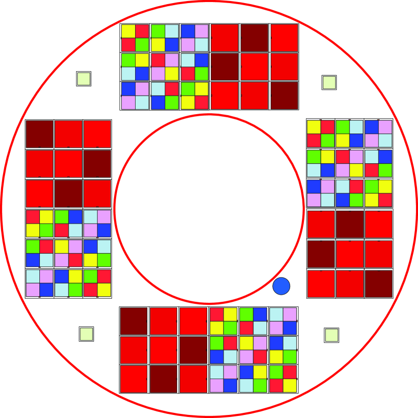
Figure 1: The layout of detectors on the SNAP focal plane. Each $17.5\times 17.5$ square arcminute CCD bank contains a $6\times 6$ array of optical filters. Each infrared HgCdTe bank contains a $3\times 3$ array with the same area. The total area of the detectors is 0.7 square degrees. The inner annulus has a radius of 0.06 radians ($0.34^{\circ}$) and the outer annulus has a radius of 0.013 radians ($0.74^{\circ}$). The spectrograph optical port is the small circle in the lower right quadrant. The four small squares are star guiders.

The SNAP CCDs and HgCdTe detectors are arranged in an annulus in the SNAP focal plane. As shown in Figure 1, there are four banks of CCDs and four banks of HgCdTe detectors. Each bank of CCDs consists of an array of $3\times 3$ CCDs. Each CCD is then covered by a $2\times 2$ grid of optical filters, in quarters of different colors. Thus, each CCD bank is a $6\times 6$ array of optical filters. The pattern of colors is arranged so that as the telescope is slewed across the sky either horizontally or vertically, each patch of sky will be viewed through all 6 optical filters in turn. A step-and-stare technique, whereby the telescope is slewed repeatedly by the angular size of one optical filter ($\sim 3^{\prime}$), accumulates an image in all bands without recourse to a moving filter wheel.

Adjacent on the focal plane, the HgCdTe detectors are in $3\times 3$ arrays, with each detector covered entirely by just one NIR filter (H’, J or K). Conveniently, since each of the NIR filters is four times the area of a single optical filter, the stacked NIR exposures in each sweep are twice as long as the optical exposures. As before, these filters are also arranged so that one sweep will observe the same survey area in all the filters, save for edge effects (the first and last fields in the sweep direction will not be observed in both the infrared and optical bands).

4 Survey Strategy

4.1 Deep Survey

Approximately 60% of the observing time in the two 16 month supernova campaigns will be spent on photometry. A total of 15 square degrees (7.5 square degrees in each campaign) will be scanned once every four days, stepping through all of the nine filters. Over the course of the deep survey, the total integration time will be 144,000 seconds in each optical filter and twice that in each infrared filter. The remaining 40% of the time will be spent using the spectrograph to observe approximately 1000 supernovae per field (2000 total supernovae) that will be detected out to $z\approx 1.7$. During spectroscopy, the imagers will be left switched on and any coincidental further integration within the survey region will be in addition to these numbers.

The deep survey will be useful for several weak lensing studies. The extremely high number density of resolved background galaxies ($\sim 260$ per square arcminute), each with a local shear estimator, samples the lensing field with very high resolution. As described in paper II, this can be converted into a detailed two-dimensional (projected) map of the mass distribution which shows clusters, filaments, and structure down to the scale of galaxy groups. The nine filters will provide photometric redshifts for almost all these galaxies, accurate to $\Delta z\approx 0.02$ (paper II). This will allow the subdivision of the detected galaxies into redshift bins in order to trace the evolution of the mass power spectrum. Furthermore, recent theoretical developments make possible a direct inversion of the shear distribution, simultaneously taking into account all the redshift information ([17]; [18]; [19]; paper II). Using this technique, mass maps can also be created directly in three dimensions. As discussed in paper II, a mass-selected cluster catalogue can then be extracted from these maps. Using the SNAP deep survey, this will result in a fine mass resolution even at reasonable distances. Along with cosmological probes, such a catalog can test astrophysical processes and the hypothesis of structure formation via gravitational instability.

4.2 Wide Survey

The SNAP mission will also include a 5 month wide survey designed primarily for weak lensing. This is the survey that will allow us to use weak lensing to put constraints on cosmological parameters. This survey will also be useful for a variety of other studies requiring high resolution wide field multi-band imaging.

4.2.1 Instrumental Constraints

The minimum exposure time of SNAP is constrained by the amount of solid–state storage on the spacecraft and the ability of the spacecraft to download data. These two constraints have been set at 350 GB of storage which can be downloaded once every 3 day orbit. This limits exposure times to 500 seconds or longer if all filters are to be used and only lossless on-board compression is done. Because this data set will be of great use to the larger astronomical community, and we will utilize all nine bands to calculate photometric redshifts for the source and lens galaxies, we opt to collect data in all 9 bands and not to further compress the data on-board. SNAP will be able to perform a slew and a CCD/HgCdTe readout in about 30 seconds. Thus, our de facto time between exposures will be 530 seconds.

Each CCD bank consists of 9 CCDs, each with $3510\times 3510$ pixels. Each pixel is 0.1 arcseconds square. All four CCD banks thus provide

$$4\times 9\times(3510)^{2}\times(0.1^{\prime\prime})^{2}=0.34\textrm{ deg}^{2}$$

of survey area. As with any high-orbit space mission, a high rate of cosmic rays has been budgeted for in the SNAP orbit, and we will need to take four dithered exposures at each pointing. These will be dithered by a small (a few pixels) non-integer pixel value. A small dither is optimal for removing cosmic rays/pixel defects; and the non-integer pixel value allows for later “DRIZZLEing” to increase image resolution [20]. To cover each filter in the bank, we need to step the telescope six times (either horizontally or vertically) by the size of the optical filters. In doing so, the infrared filters are also stepped across the field of view at the same time. Thus, the total minimum time needed for each 0.34 square degree patch is $4\textrm{(dithers)}\times 6\textrm{(filters)}\times 530\textrm{s}=12720$ seconds, or 0.147 days.

4.2.2 PSF Calibration

We will need to constantly monitor the PSF through the examination of non-saturated stars in our survey. Calibrations with a higher surface density of stars will need to be performed on occasion as well. We anticipate that we will need to perform this calibration at least at the beginning and end of our survey, and each time there is a focus change in the telescope. The calibration will be done by pointing at a stellar field (such as a globular cluster, and open cluster or a low galactic latitude field), and taking 4 dithered images for each CCD bank. There are four banks of CCDs, requiring $4\times 4\times 530\textrm{ seconds}=0.1$ days for each full PSF calibration. The predicted observing efficiency of the telescope is 86% including the time needed for downloading data and time spent not observing while passing through radiation zones. If we estimate that we will need to perform one calibration every 2 months, this requires less than 0.2% of the telescope time during a weak lensing survey. Thus, we estimate that approximately 85% of the time allotted to a weak lensing survey will be used to gather data.

4.2.3 Survey Characteristics

Given 85% efficiency, it takes 0.17 days to observe a 0.34 square degree patch. Therefore, we can observe 100 square degrees in 50 days. Paper III demonstrates that, for constraining cosmological parameters with lensing, the width of the survey is more important than its depth. We therefore select the minimum 500s individual integration time at the hard limit of onboard storage and download rate given in §4.2.1. Thus, given 5 months of time, or 150 days observing time, our optimal survey will be:

• 300 square degrees

• 6 optical and 3 infrared filters

• 2000 seconds integration in each optical filter

• 4000 seconds integration in each infrared filter

• 4 dithers to improve resolution and eliminate cosmic rays

2000 seconds of exposure time allows us to reach a 5$\sigma$ point source detection limit for an object with 27.5 in $I$ and 28.0 in $V$. For a 10$\sigma$ detection of an extended galaxy with an exponential profile, as is relevant to weak lensing, these limits drop to isophotal magnitudes of 26.0 and 26.4 respectively.

According to paper II, this depth allows us to measure the shapes of $\sim 120$ galaxies per square arcminute in the $I$ band. Photometric redshifts can be calculated for almost all of these with an error of $\Delta z\approx 0.05$. Co-adding 2 or more of the bands will allow a deeper study with a higher surface density of galaxies. Further simulations are underway to quantify the gains available using field co-addition.

5 Systematic Effects

The primary goal of a weak lensing survey is to measure the shapes of as many galaxies as possible as accurately as possible. The size, anisotropy, and temporal stability of a telescope’s PSF are the most important factors in determining the number density of galaxies that can be measured and the accuracy with which the shapes can be ascertained. In order to accurately measure galaxy shapes and sizes, it is necessary to remove the effects of telescope PSF and detector induced shear from the galaxy images.

5.1 Contributions to the PSF

In Table 1 we identify 8 effects which will contribute to the PSF and the sizes of those effects. The sizes and shapes of the effects are estimates using SNAP engineering models, but will be present in any wide field space based mission. The one dimensional rms contributions from each source are listed in arcseconds. For circularly symmetric patterns, the contribution is the projection of the distribution onto the $x$ or $y$ axis. For more complicated distributions, it is 71% of the root sum square of the two axes. The purpose of this section is to discuss these effects and their time variability to determine how they impact weak lensing measurements.

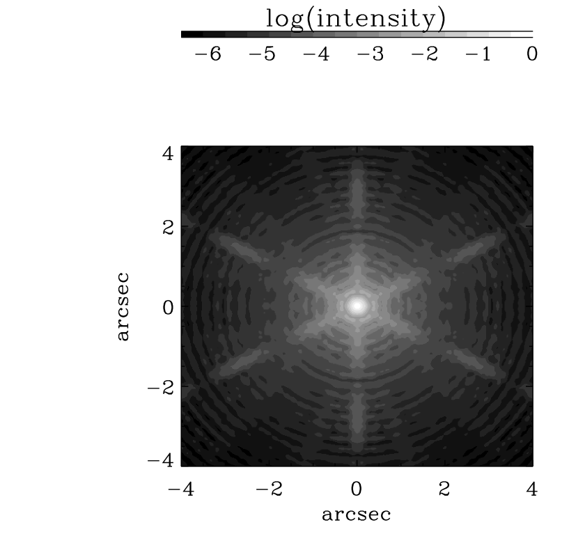
Figure 2: Oversampled image of the SNAP PSF at 800nm. The image is 8 arcseconds (80 SNAP pixels) on a side. Note the logarithmic intensity scale.

We have created model PSFs across the SNAP field of view (FOV) taking into account some of these effects (see figure 2). These models will be used to study how small perturbations of the SNAP telescope design and operating conditions will affect the PSF. The first three items in Table 1 (diffraction, diffusion, and ideal geometric aberrations) are included in the PSF models discussed below. These are the most important contributions to the optical PSF.

Item 4 (attitude control system jitter) is difficult to model because the sources of telescope jitter are stochastic events caused by many different processes. The effects of jitter will have to be measured via stellar images in orbit. Items 5 and 6 (mirror manufacturing and alignment errors) are not possible to predict, but also can be corrected with stellar images after SNAP has been launched. In §5.5, we show how slight perturbations in mirror alignment will affect the PSF.

Item 7 (charge transfer efficiency; CTE) is a detector effect. Electron traps within the semiconductor array are created by high energy cosmic ray hits, and cause charge trailing during CCD readout. This can falsely elongate all objects in the readout direction. The magnitude of the effect can vary across the CCD, and CTE is known to degrade over the lifetime of the mission (see §5.6). Tests indicate that the CTE in the Berkeley designed CCDs being used for SNAP will be quite small and the degradation will be significantly less than is seen on HST [21] and [22]. There will not be a CTE effect on the NIR detectors. As long as the small CTE effects are linear, this small effect should be correctable in software using data taken in orbit.

Item 8 (silicon transparency) is also referred to as “red defocus.” This contributes only about 1 micron (0.01 arcseconds) to PSF size at a wavelength of 800nm, and less at shorter wavelengths . Red defocus is a consequence of the fact that blue light is absorbed at the surface of the CCD while red light is absorbed throughout the thickness of the CCD. Thus, there is no optimal focal plane for red light. This is only a problem in the extreme red ($>800$nm) and thus does not effect galaxy shape measurements done using optical wavelengths.

5.2 PSF Simulations

We have developed an IDL routine to model the SNAP PSF across the SNAP field of view. The PSF model takes into account three of the effects in Table 1: diffraction from the struts and the aperture (item 1), Gaussian charge diffusion within the CCDs (item 2), and the spot diagram (ray tracing through the optics; item 3). We use the currently planned technical specifications for SNAP. The simulations are based on a primary mirror radius of 1 meter, a secondary structure obscuration of radius 0.4 meters (the secondary mirror itself has radius 0.225 meters), 3 supporting struts of 4 cm thickness, and a distance of 2.1 meters between the primary and secondary mirrors. A CCD diffusion value of 4.0 $\mu$m RMS is used. We use a fiducial wavelength of 800 nm to test the effects on the PSF of perturbations of several SNAP parameters. Below, we explore the dependence of PSF on wavelength for optical wavelengths. We do not explore the infrared PSF because infrared images will not be used to measure galaxy shapes.

Figure 2 shows an oversampled PSF created a distance of 0.01 radians ($0.57^{\circ}$) from the optical center of the SNAP FOV, with an input wavelength of 800 nm. The image measures approximately $8\times 8$ arcseconds. The PSF shows a nearly-circular central core as well as the extended diffraction pattern caused by the struts and the aperture. Figure 3 shows the average radial profile of this PSF. The PSF intensity drops to 10% of the central value within 0.2 arcseconds or 2 SNAP pixels. This figure also demonstrates the improvement in PSF size of a space-based telescope over the best ground-based PSF consistently available.

5.3 PSF Size

The size of the PSF is crucial for weak lensing because only resolved galaxies, with sizes larger than the PSF, can provide useful shape or size information. Figure 4 shows the PSF size as a function of wavelength. The size shown is the FWHM of a Gaussian fit to the PSF by the IDL procedure Gauss2dfit. Because the size of the PSF increases with increasing wavelength, it would be advantageous for us to measure galaxy shapes with a short wavelength. However, a higher surface density of galaxies can be imaged in redder filters than in bluer filters. This is an issue that will be optimized using the simulations described in paper II. Figure 4 also shows the size of a diffraction limited PSF. Clearly, the SNAP PSF size is not diffraction limited and is dominated by charge diffusion and other factors.

The rms value of charge diffusion by electrons in CCDs is driven by the applied voltage and the thickness of the fully depleted CCD. A higher applied voltage, or a thinner CCD, results in a lower value of charge diffusion, benefitting the PSF. On the other hand, a higher voltage or a thinner CCD produces a smaller manufacturing yield, a higher failure rate, and less quantum efficiency towards extreme red wavelengths. However, as the allowed diffusion value increases, the size of the PSF increases almost linearly, as shown in figure 5. There will be a detailed trade-off study done to determine what value of diffusion strikes the proper balance between mission risk, cost, and weak lensing capability. Current SNAP specifications call for a charge diffusion of $4~{}\mu$m.

5.4 PSF Anisotropy

The lensed shapes of galaxies that we are trying to measure are unfortunately altered again during observation. Instrumental effects within a telescope must be undone during data reduction in order to recover the true image shapes and the lensing-induced ellipticity (or polarization). The two main detector effects are smear, or PSF convolution, and shear, which includes astrometric distortions.

Smearing tends to limit the size of the smallest galaxies able to be measured: size and shape information for galaxies smaller than the PSF is lost during convolution. The isotropic component of the PSF circularizes galaxies, while an anisotropic component may also cause galaxies to become preferentially elongated in one direction. Another important factor affecting the measured image shapes is distortion from the detector. Such astrometric distortions precisely mimic shear by weak gravitational lensing. Detailed analysis of the SNAP detectors’ geometric distortion awaits more advanced detector models and ground measurements of the detectors themselves. Fortunately, the small shear distortions predicted for SNAP should be straightforward to subtract, using measurements of the astrometric shifts of dithered stellar images. Furthermore, detector distortion affects only the shape of the measured objects, rather than the size. Thus, this effect is not a limiting factor in the size of galaxies which can be measured.

Several techniques have been developed to correct image shapes for both of smear and shear using software, including KSB [23], RRG [24] and “shapelets” [25] [26]; see also a related method by [27]. To measure the ellipticity of the PSF we first calculate the intensity weighted second moments $I_{xx}$, $I_{yy}$ and $I_{xy}$. These are defined as the following sum over pixels (i)

$$I_{xy}=\frac{\sum_{i}I(x_{i},y_{i})x_{i}y_{i}w(x_{i},y_{i})}{\sum_{i}I(x_{i},y_{i})}$$ (1)

where $I(x,y)$ is the intensity in a pixel, $x$ and $y$ are the distances from that pixel to the centroid of the PSF and $w(x,y)$ is a Gaussian weighting function with a standard deviation of 0.2 arcseconds (two SNAP pixels). Similar equations hold for $I_{xx}$ and $I_{yy}$. Following lensing convention, the two-component ellipticity $e_{i}$ is defined as

$$e_{1}=\frac{I_{xx}-I_{yy}}{I_{xx}+I_{yy}}\hskip 28.45274pte_{2}=\frac{2I_{xy}}{I_{xx}+I_{yy}}.$$ (2)

Measured ellipticities can then be corrected for instrumental distortion using higher order weighted moments, and the moments of the PSF (see e.g. [24]).

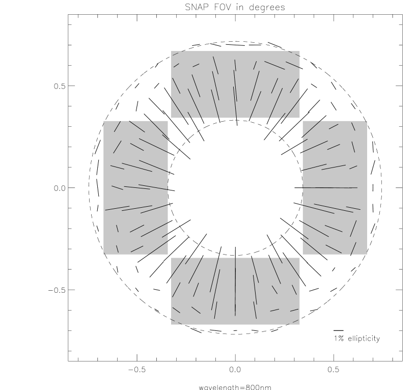
Figure 6: The PSF induced ellipticity over the SNAP FOV at 800 nm. Each line represents the size of the ellipticity that the PSF induces in a point–like source at that position. This ellipticity field is wavelength dependent so the actual measured PSF would depend on the fixed filter at a given position.

Figure 6 shows the ellipticity of the SNAP PSF over the SNAP field of view produced by the first three factors listed in Table 1 at a wavelength of 800 nm. The size of the PSF induced ellipticity is not large, roughly 4–5 % at most. For comparison, the PSF induced ellipticity of WFPC2 on HST is up to 10%, as measured empirically [24] and calculated using the program TINYTIM [28]. The PSF does change over the focal plane and in fact over a single CCD detector. Therefore, a much finer grid of model PSFs would be needed to accurately model the SNAP PSF over the entire focal plane.

5.5 Mirror Misalignment

The above PSF simulations were performed assuming a perfect mirror alignment. The effects of a simple mirror misalignment can be added to the simulations by creating a new spot diagram for the misaligned mirrors. Such a misalignment may occur due to thermal fluctuations in the barrel of the telescope, and particularly in the secondary mirror support struts. SNAP engineering estimates indicate that the mirror alignment error will be at maximum $\theta=2\times 10^{-4}$ degrees. Most likely the mirror misalignment would be only half of that.

Figures 7 and 8 show the change in the induced ellipticity caused by mirror alignment errors of 1 and $2\times 10^{-4}$ degrees, respectively. These plots indicate how much the induced ellipticity would differ from the nominal perfectly aligned mirrors in figure 6, and as such are shown for a wavelength of 800nm. These plots represent the maximum error SNAP would face if the mirrors become misaligned and no correction is made to galaxy shapes for the misalignment. This error manifests itself as a residual post-correction rms ellipticity $\langle(\Delta e)^{2}\rangle^{\frac{1}{2}}$ where $\Delta e$ is the difference in ellipticity $e=\sqrt{(e_{1}^{2}+e_{2}^{2})}$ of the PSF between the aligned and misaligned mirrors, and the angle brackets indicate an average over the SNAP FOV. This residual ellipticity is 0.5% for a mirror alignment error of $10^{-4}$ degrees and 0.9% for an alignment error of $2\times 10^{-4}$ degrees. For comparison, the typical residual ground-based post-correction ellipticity is 5-10%. Thus, in the worst-case scenario when a mirror alignment error goes unnoticed, this effect will only introduce an error five to ten times smaller than that found in ground-based images. Vigilant monitoring of the SNAP PSF will allow us to correct for mirror misalignment and reduce this error.

5.6 Other Sources of Time Variability

The time variability of the PSF is a concern because of the accuracy to which object shapes need to be measured for weak lensing. The HST’s PSF changes significantly in time periods of order days and even changes during the course of its ninety minute orbit [29] [24], hindering corrections for instrumental shape distortions. In addition to possible mirror misalignment errors discussed above, SNAP will suffer from some amount of “structural dryout creep” which is an outgassing of water from carbon fiber elements of the optical support structure. The optical supports will shrink as this outgassing occurs, but this is expected to last only a few months and then stabilize. During this initial phase, the telescope will be refocused to bring the PSF back to its nominal value but the PSF will drift away from that value as the telescope goes out of focus.

There will also be an initial thermal contraction for several months, and possible “creaking” of the detector support structure, as the telescope cools after launch. Thus, this will not be the optimal time for weak lensing measurements. Throughout its lifetime, the spacecraft will also undergo further thermal contraction and expansion cycles as the solar exposure changes during its orbit. The currently planned highly elliptical orbit will minimize this effect, but the consequences upon the PSF will have to be monitored by examining stellar data.

The charge transfer efficiency (CTE) of CCDs is known to degrade over time, as cosmic ray hits create electron traps within the semiconductor array. These traps will cause image trailing during CCD readout, falsely elongating all the galaxies in the readout direction. This is clearly a concern for weak lensing. With this in mind, the SNAP CCDs are being specifically designed to undergo minimal CTE degradation.

5.7 PSF Based Survey Requirements

Based on the above analysis of the SNAP PSF, we plan the following for a weak lensing survey:

1. The wide field weak lensing survey should not be conducted within the first several months of launch

2. Galaxy shapes should be measured with a filter at $\sim 800$ nm or shorter to utilize the smaller PSF

3. Stellar images (in low Galactic latitude fields) should be taken at regular intervals to monitor and correct for the PSF

4. Astrometric shifts of stars should be used to calculate detector distortion early in the mission

5. Aim for 4.0 $\mu$m diffusion or less as a trade-off between mission risk, cost, and PSF size

6 Conclusions

A wide field space telescope is crucial in the drive to understand both dark energy and dark matter. We have studied the systematic effects contributing to the PSF of such a telescope. The PSF can be designed to be much smaller than the best available from the ground, and more stable over time than ground-based PSFs or even that of the HST. These high quality image specifications ensure that a telescope like SNAP will be a powerful instrument for the next generation of precision weak lensing experiments. We have outlined baseline survey strategies that will lead to exciting new lensing results.

Paper II introduces simulations of space-based images that are being used to predict the sensitivity to weak gravitational lensing, using the specifications presented here. That paper includes the accuracy and resolution of possible dark matter maps. Paper II also contains a calculation of the accuracy of photometric redshifts in SNAP data. These numbers are then applied in paper III to determine how well wide field space based observations will be able to constrain cosmological parameters including the dark energy equation of state parameter w.

JR was supported by an NRC/GSFC Research Associateship. AR was supported in Cambridge by an EEC fellowship from the TMR network on Gravitational Lensing, by a Wolfson College Research Fellowship, and by a PPARC advanced fellowship. We thank the Raymond and Beverly Sackler Fund for travel support. We thank the anonymous referee and Douglas Clowe for useful suggestions.

Figure 3: The averaged radial profile of the SNAP PSF at 800 nm (boxes). The curve is a Gaussian with FWHM 0.55 arcseconds, the best seeing consistently available with the Keck Telescope on the ground.

Figure 4: The FWHM of a Gaussian fit to the SNAP PSF as a function of wavelength (boxes). The solid line is a diffraction limited PSF for the 2 meter SNAP primary mirror. The sizes of the effects of diffusion and aberrations are also shown.

Figure 5: The FWHM of a Gaussian fit to the SNAP PSF as a function of the rms charge diffusion by electrons in the CCD. Higher values of diffusion are safer and less costly to achieve, but lead to larger PSFs. The horizontal line shows the FWHM of the PSF in the limit of no charge diffusion or other factors (the diffraction limit). The vertical line represents the default value of diffusion we use in our simulations. These values assume a wavelength of 800nm.

Figure 7: The change in the PSF induced ellipticity between the ideal mirror alignment and a situation in which the secondary mirror alignment is tilted by $\theta=10^{-4}$ degrees.

Figure 8: Same as figure 7 but with a mirror tilt of $\theta=2\times 10^{-4}$ degrees.

Table 1: Model Contributions to the SNAP PSF.

#	Effect	Size of PSF Contribution
1	optical diffraction	circular Airy disk 0.06 arcsec RMS at 1000 nm
2	electron diffusion	circular Gaussian 0.04–0.05 arcsec RMS
3	ideal geometric aberrations	blobs 0.02–0.03 arcsec RMS
4	attitude control system jitter	circular Gaussian 0.02 arcsec RMS
5	mirror manufacturing errors	circular Gaussian 0.02 arcsec RMS
6	mirror alignment errors	circular Gaussian 0.02 arcsec RMS
7	charge transfer efficiency	linear $<0.01$ arcsec
8	transparency of silicon (red defocus)	linear $<0.01$ arcsec

References

- [1] Turner, M., Physics Reports, 333, 619, 2000.
- [2] Riess, A., et al., AJ, 116, 109, 1998.
- [3] Perlmutter, S., et al., 517, 565, 1999.
- [4] Peebles, P.J.E. & Ratra, B., “The Cosmological Constant and Dark Energy,” astro-ph/0207347, 2002.
- [5] Turner, M., et al., “Connecting Quarks With the Cosmos: 11 Science Questions for the New Millenium,” National Academies Press, 2002.
- [6] Massey, R., et al., “Weak Lensing from Space II: Dark Matter Mapping,” 2003, AJ submitted, paper II.
- [7] Refregier, A., et al.,“Weak Lensing from Space III: Cosmological Parameter Estimation,” 2003, SJ submitted, paper III.
- [8] Mellier, Y., et al., “Astronomy, Cosmology and Fundamental Physics”, ESO-CERN-ESA Symposium. P. A. Shaver, L. Di Lella, and A. Gimenez Eds., 2002.
- [9] Jain, B., ApJ, 580, L3, 2002.
- [10] Alcock, C.,et al., 2003, in preparation
- [11] Aldering, G., et al., “Overview of the SuperNova/Acceleration Probe” Proc SPIE v.4835 paper 21, 2002, astro-ph/0209550.
- [12] Kim, A., et al., “Wide-Field Surveys from the SNAP Mission” Proc SPIE 4836 paper 10 2002, astro-ph/0210077.
- [13] Lampton, M., et al., “SNAP Telescope” Proc SPIE v.4849 paper 29 2002a, astro-ph/0209549.
- [14] Lampton, M., et al., “SNAP Focal Plane” Proc SPIE v.4854 paper 80 2002b, astro-ph/0210003.
- [15] Tarle, G., et al., “The SNAP Near IR Detectors” Proc SPIE v.4850 paper 131 2002, astro-ph/0210041.
- [16] Perlmutter,S. et al, 2002, http://snap.lbl.gov
- [17] Taylor, A., asto-ph/0111605, 2001.
- [18] Hu W., Keeton C., 2002, astro-ph/0205412
- [19] Bacon, D., & Taylor, A, 2003, MNRAS in press, astro-ph/0212266.
- [20] Fruchter A. S. & Hook R. N. 2002, PASP, 114, 144.
- [21] Bebek, C.J., Groom, D. E., Holland, S. E., Karchar, A., Kolbe, W. F., Levi, M. E., Palaio, N. P., Turko, B. T., Uslenghi, M. C., Wagner, M. T. & Wang, G., “Proton radiation damage in high-resistivity n-type silicon CCDs,” Proc. SPIE Vol. 4669, April 2002, p. 161-171.
- [22] Bebek, C.J., Groom, D. E., Holland, S. E., Karchar, A., Kolbe, W. F., Lee, J. Levi, M. E., Palaio, N. P., Turko, B. T., Uslenghi, M. C., Wagner, M. T. & Wang, G., “Proton radiation damage in p-channel CCDs fabricated on high-resistivity silicon,” IEEE Transactions on Nuclear Science, Volume: 49 Issue: 3, Jun 2002 p.1221–1225.
- [23] Kaiser, N., Squires, G., & Broadhurst, T. 1995, ApJ, 449, 460.
- [24] Rhodes,J., Refregier, A., & Groth, E.J., ApJ, 536, 739, 2000.
- [25] Refregier, A., 2003, MNRAS, 338, 35R.
- [26] Refregier, A. & Bacon, D., 2003, MNRAS, 338, 48R.
- [27] Bernstein, G. & Jarvis, M., 2002, AJ, 123, 583.
- [28] Krist, J. & Hook, R., “ The TinyTim User’s Guide”, STScI, 2003.
- [29] Hoekstra, H., et al., ApJ, 504, 636, 1998.