Weak Lensing from Space III:
Cosmological Parameters

Abstract

Weak gravitational lensing provides a unique method to directly map the dark matter in the universe and measure cosmological parameters. Current weak lensing surveys are limited by the atmospheric seeing from the ground and by the small field of view of existing space telescopes. We study how a future wide-field space telescope can measure the lensing power spectrum and skewness, and set constraints on cosmological parameters. The lensing sensitivity was calculated using detailed image simulations and instrumental specifications studied in earlier papers in this series. For instance, the planned SuperNova/Acceleration Probe (SNAP) mission will be able to measure the matter density parameter $\Omega_{m}$ and the dark energy equation of state parameter $w$ with precisions comparable and nearly orthogonal to those derived with SNAP from supernovae. The constraints degrade by a factor of about 2 if redshift tomography is not used, but are little affected if the skewness only is dropped. We also study how the constraints on these parameters depend on the survey geometry and define an optimal observing strategy.

1 Introduction

Weak gravitational lensing provides a unique method to directly map the distribution of mass in the universe (for reviews see Bartelmann & Schneider 2001; Mellier et al. 2002; Hoekstra et al. 2002; Refregier 2003). The coherent distortions that lensing induces on the shape of background galaxies have now been firmly measured from the ground and from space. The amplitude and angular dependence of this ‘cosmic shear’ signal can be used to set strong constraints on cosmological parameters. Several surveys are now in progress to map larger areas and thus reduce the uncertainties in these parameters. However, future ground based surveys will eventually be limited by the systematics induced by atmospheric seeing. Space based observations do not suffer from this effect, but their statistics are currently limited by the small field of view of existing space telescopes.

In this paper series, we study how these limitations can be circumvented using wide field imaging from space, using the planned SuperNova/Acceleration Probe (SNAP) mission (Perlmutter et al. 2003) as a concrete example. In the first paper in this series (Rhodes et al. 2003; Paper I), we study the instrumental characteristics and survey stategy of such a mission, showing that it would provide both excellent statistics and reduced systematics relevant for weak lensing. In a subsequent paper (Massey et al. 2003; Paper II), we used detailed image simulations to compute the sensitivity for measuring the weak lensing shear from space, and thus to derive high resolution maps of the Dark Matter in the local universe.

In this paper, we use the previously derived lensing sensitivity (see Papers I and II) to determine the constraints that can be placed on cosmological parameters via weak lensing from space. We consider quintessence (QCDM) models with a dark energy component with arbitrary constant equation of state parameter $w$. We compute the lensing power spectrum and skewness and their associated errors for different survey strategies. We study how the photometric redshifts derived from the SNAP filter set can be used to study the evolution of the lensing power spectrum. We then compare the resulting lensing constraints on cosmological parameters with those derived from supernovae. Earlier studies of the constraints on dark energy from generic weak lensing surveys can be found in Hui (1999), Huterer (2001), Benabed & Bernardeau (2001), Hu (2001), Weinberg & Kamionkowski (2002), Munshi & Wang (2002). While these authors have considered generic weak lensing surveys, we use realistic redshift distributions, lensing sensitivities, and photometric-redshift errors relevant for the concrete case of SNAP. This allows us to include the effects of photometric-redshift errors and leakage between redshift bins, and to study the trade off between width and depth in future surveys. We also study how the measurement of the skewness can be combined with power spectrum tomography to improve the accuracy of the determination of cosmological parameters.

This paper is organized as follows. In §2, we summarize the characteristics of the SNAP mission. In §3, we describe its capabilities for deriving photometric redshifts. In §4, we describe the cosmological models we will consider. In §5, we compute the lensing power spectrum, its associated errors, and its redshift evolution. In §6, we compute the skewness of the shear field and associated errors. In §7, we compute the constraints which can be set on cosmological parameters from measurements of the power spectrum and skewness. Our conclusions are summarized in §8.

2 The SNAP Mission

The SNAP satellite will consist of a 2 meter telescope in space with a field of view of 0.7 deg² (Perlmutter et al. 2003; see also Paper I). The mission lifetime will be divided between two deep 16 months survey and a 5 month wide survey. The deep surveys will cover 15 deg² and are primarily designed for the search for Type Ia supernovae. It will also be invaluable to map the dark matter via weak lensing (see Paper II). The wide survey is designed primarily for weak lensing and will cover 300 deg². The spacecraft will be in a high elliptical orbit with good thermal stability, thus affording stable image quality and a low level of systematics. The details of the performance of the instrument for weak lensing and of the survey strategy can be found in Paper I.

Table 1: Survey parameters and redshift distributions

Survey	$z$-bins	$t_{\rm exp}$	$t_{\rm tot}$	$A$	$n_{g}$	$\sigma_{\gamma}$	$z_{m}$	$z_{0}$	$\alpha$	$\beta$	$z_{+}$	$\zeta_{+}$	$z_{-}$	$\zeta_{-}$
		(sec)	(months)	(deg2)	(amin-2)
Deep		20000	32	15	260	0.36	1.43	1.31	2.00	2.00
Wide		2000	5	300	100	0.31	1.23	1.13	2.00	2.00
	1/2	2000	5	300	50	0.31	0.96	1.32	1.94	3.38	1.36	0.042
	2/2	2000	5	300	50	0.31	1.73	1.51	0.53	2.16			1.36	0.048
	1/3	2000	5	300	33	0.31	0.81	1.13	1.95	5.55	1.11	0.031
	2/3	2000	5	300	33	0.31	1.31	0.80	20.07	3.45	1.11	1.515	1.59	1.515
	3/3	2000	5	300	33	0.31	1.93	1.57	1.50	2.48			1.59	0.042
Wide+		1000	5	600	68	0.30	1.17	1.07	2.00	2.00
Wide$-$		4000	5	150	150	0.33	1.31	1.20	2.00	2.00

3 Photometric Redshifts

The SNAP focal plane will be partially covered by CCDs sensitive to 9 optical and near–IR bands. Paper II describes how this filter set affords excellent photometric redshifts. This was tested using the HyperZ code (Bolzonella et al. 2000) to generate simulated galaxy spectra and recovered photometric redshifts. Using all nine filters, we found that redshifts can be recovered with a $1\sigma$ precision better than 0.03. Including the near–IR detectors prevents catastrophic failures in redshift estimation by eliminating strong degeneracies between low ($z\lesssim 0.5$) and high ($z\gtrsim 1$) redshift bins (see Paper II).

These high precision photometric redshifts will allow us to construct 3-dimensional maps of the dark matter (see Paper II). They will also be useful to study the evolution of the lensing statistics. Figure 1 shows how photometric redshifts can be used to group galaxies into redshift bins. The input redshift distribution $n(z)$ was assumed to have the form

$$n(z)\propto z^{\alpha}e^{-(z/z_{0})^{\beta}}$$ (1)

where $z_{0}$, $\alpha$ and $\beta$ are parameters estimated from existing deep redshift surveys (see Paper II). Table 1 lists the values of these parameters for the deep and wide surveys, along with the associated median redshift $z_{m}$, the surface density $n_{g}$ of galaxies usable for lensing, and the survey solid angle $A$. The exposure time $t_{\rm exp}$ for each optical filter, along with the total observing $t_{\rm obs}$ time for the survey are also listed. The figure shows the redshift distribution resulting from binning the galaxies into 2 and 3 photometric-redshift bins, with approximately the same number of galaxies in each bin. With the near–IR detectors (left panels), the photometric redshifts afford excellent separation between the bins. In the absence of these detectors (right panels), the leakage between bins degrades, due to the increased noise and degeneracies in the photometric redshifts (see Figure 7 in Paper II). In the following, we will always assume that the near–IR detectors are available.

The redshift distributions of each bin can be described analytically by multiplying the input redshift distribution $n(z)$ in equation (1) by the high-$z$ and low-$z$ filter functions $f_{+}(z)$ and/or $f_{-}(z)$ given by

$$f_{\pm}(z)=\left[1+e^{\pm(z_{\pm}-z)/\zeta_{\pm}}\right]^{-1},$$ (2)

where $z_{+}$ and $z_{-}$ are the cut off redshifts, and $\zeta_{+}$ and $\zeta_{-}$ are smearing factors arising from the finite photometric redshift accuracy. Fits to the redshift bin distributions using these analytical forms are shown in Figure 1. The values of the resulting parameters for 2 and 3 redshift bins are listed in Table 1. In §5.3, we study how multiple redshift bins can be used to measure the evolution of the lensing power spectrum and thus improve the accuracy of the measurement of cosmological parameters.

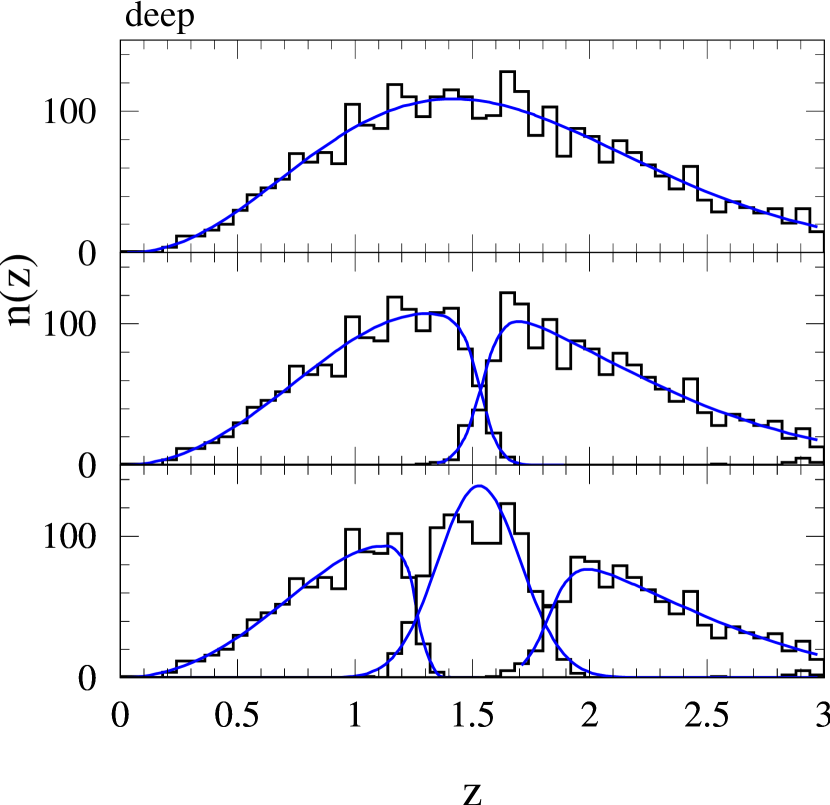
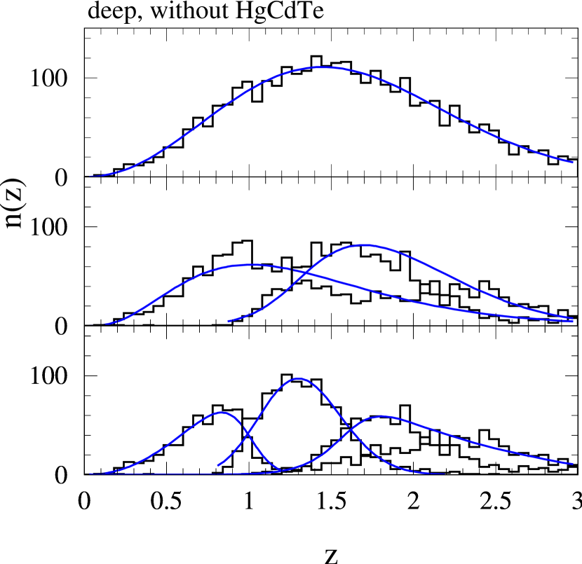
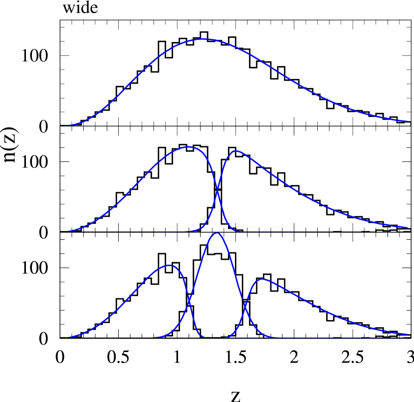
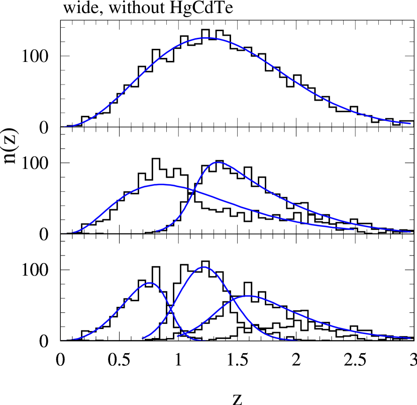
Figure 1: Redshift bins derived from photomotric redshifts. In each of the 4 panels, the histograms show the redshift distributions resulting from cuts in photometric redshifts aimed to produce 1,2 and 3 redshift bins from top to bottom, respectively. The solid curves correspond to fits for the analytical form of equations (1-2). The top and bottom panels correspond to the deep and wide SNAP surveys respectively. In the left panels, the full set of 9 optical and near–IR (HgCdTe) SNAP filters were used to estimate the photometric redshifts. In the right panels, only the 6 optical filters were used. In all cases, the normaliszation is arbitrary.

4 Cosmological Model

We consider a cosmology with an expansion parameter $a=(1+z)^{-1}$ that is determined by a matter component and a dark energy (or ‘quintessence’) component with present density parameters $\Omega_{m}$ and $\Omega_{q}$, respectively. The equation of state of the dark energy is parametrized by $w=p_{q}/\rho_{q}$, which we assume to be constant and is equal to -1 in the case of a cosmological constant. The evolution of the expansion parameter is given by the Hubble constant $H$ through the Friedmann equation

$$H=\frac{\dot{a}}{a}=H_{0}\left(\Omega_{m}a^{-3}+\Omega_{q}a^{-3(1+w)}+\Omega_{\kappa}a^{-2}\right)^{\frac{1}{2}},$$ (3)

where $\dot{a}=da/dt$ and the total and curvature density parameters are $\Omega$ and $\Omega_{\kappa}=1-\Omega$, respectively. The present value of the Hubble constant is parametrized as $H_{0}=100h$ km s^-1 Mpc^-1.

As a reference model, we consider a fiducial $\Lambda$CDM model with parameters $\Omega_{m}=0.30$, $\Omega_{b}=0.047$, $n=1$, $h=0.7$, $w=-1$, consistent with the recent WMAP experiment (see tables 1-2 in Spergel et al. 2003). In agreement with this experiment, we assume that the universe is flat, i.e. that $\Omega=\Omega_{m}+\Omega_{q}=1$. (Note that, in our notation, $\Omega_{m}$ includes both dark matter and baryons). The shape parameter for the matter power spectrum is taken to be $\Gamma=\Omega_{m}h\exp{[-\Omega_{b}(1+\sqrt{2h}/\Omega_{m})]}$ as prescribed by Sugiyama (1995). The matter power spectrum is normalized according to the COBE normalization (Bunn & White 1996), which corresponds to $\sigma_{8}=0.88$. This is consistent with the WMAP results (Spergel et al. 2003) and with the average of recent cosmic shear measurements (see compilation tables in Mellier et al. 2002; Hoekstra et al. 2002; Refregier et al. 2003). In the following, we will consider deviations from this reference model.

5 Weak Lensing Power Spectrum

5.1 Theory

The weak lensing power spectrum is given by (eg. Bartelmann & Schneider 1999; Hu & Tegmark 1999; see Bacon et al. 2001 for conventions)

$$C_{\ell}=\frac{9}{16}\left(\frac{H_{0}}{c}\right)^{4}\Omega_{m}^{2}\int_{0}^{\chi_{h}}d\chi~{}\left[\frac{g(\chi)}{ar(\chi)}\right]^{2}P\left(\frac{\ell}{r},\chi\right),$$ (4)

where $r(\chi)$ is the comoving angular diameter distance, and $\chi_{h}$ corresponds to the comoving radius to the horizon. The non-linear matter power spectrum $P(k,z)$ is computed using the transfer function from Bardeen et al. (1986; with the conventions of Peacock 1997), thus ignoring the corrections on large scales for quintessence models (Ma et al. 1999). The growth factor and COBE normalization for arbitrary values of $w$ was computed using the fitting formulae from Ma et al. (1999). Considerable uncertainties remain for the non-linear corrections in quintessence models (see discussion in Huterer 2001). Here, we use the fitting formula from Peacock & Dodds (1996) but acknowledge that it differs significantly from that from Ma et al. (1999). The impact of this uncertainty is discussed below in §8.

The radial weight function $g$ is given by

$$g(\chi)=2\int_{\chi}^{\chi_{h}}d\chi^{\prime}~{}n(\chi^{\prime})\frac{r(\chi)r(\chi^{\prime}-\chi)}{r(\chi^{\prime})},$$ (5)

where $n(\chi)$ is the probability of finding a galaxy at comoving distance $\chi$ and is normalised as $\int d\chi~{}n(\chi)=1$. For our purposes, we use the analytical fits for $n(z)$ given in equations (1-2) along with the parameter values listed in table 1.

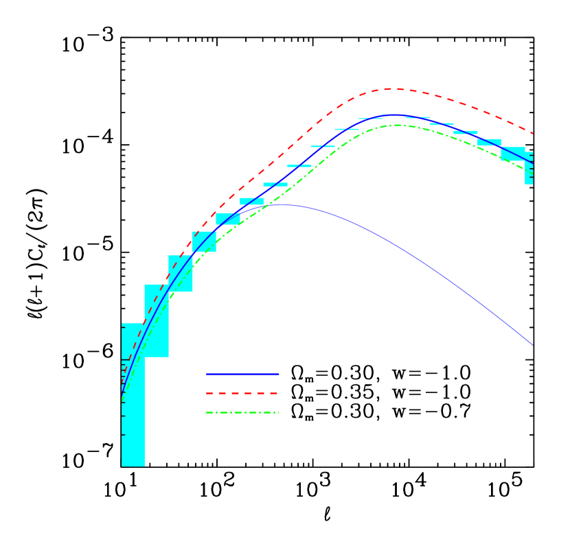
Figure 2: Weak lensing power spectrum for several cosmological models. The top solid line shows the weak lensing power spectrum $C_{\ell}$ for the fiducial $\Lambda$CDM model with $\Omega_{m}=0.30$, and $w=-1$. The bottom solid line shows the linear power spectrum for the same model. The dashed and dot-dashed lines show the nonlinear power spectra for variations of the model with $\Omega_{m}=0.35$ and $w=-.7$ respectively. In all cases, $\Omega_{q}=1-\Omega_{m}$, $h=0.7$, $\Omega_{b}=0.047$, $n=1$ and COBE normalization were assumed. The redshift distribution was taken to be that for the SNAP wide survey (unbinned) with a median redshift of $z_{m}=1.23$. The boxes correspond to the band averaged $1\sigma$ errors about the fiducial model for the SNAP wide survey (300 deg² area, 100 galaxies per arcmin² and an intrinsic shear dispersion of $\sigma_{\gamma}=0.31$).

Figure 2 shows the lensing power spectrum for the fiducial $\Lambda$CDM model. Deviations from the model corresponding to variations in $\Omega_{m}$ and $w$ are also shown. All models shown are COBE normalised. The linear power spectrum for the fiducial model is also shown, highlighting the importance of non-linear evolution for $\ell\gtrsim 100$.

5.2 Measurement uncertainties

Neglecting non-gaussian corrections, the rms uncertainty in measuring the lensing power spectrum $C_{\ell}$ is given by (Kaiser 1998; Hu & Tegmark 1999; Huterer 2001)

$$\Delta C_{l}=\sqrt{\frac{2}{(2l+1)f_{\rm sky}}}\left(C_{l}+\frac{\sigma_{\gamma}^{2}}{2n_{g}}\right),$$ (6)

where $f_{\rm sky}$ is the fraction of the sky covered by the survey, $n_{g}$ is the surface density of usable galaxies, and $\sigma_{\gamma}^{2}=\langle|\gamma|^{2}\rangle$ is the shear variance per galaxy arising from intrinsic shapes and measurement errors. Values of $\sigma_{\gamma}$ for the different SNAP surveys were derived from the image simulations in Paper II and are listed in table 1.

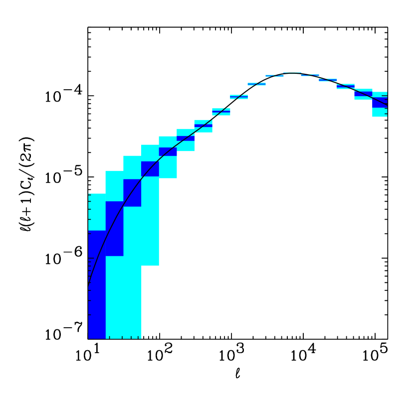
Figure 3: Measurement of the weak lensing power spectrum with the wide and deep SNAP surveys. The solid line shows the power spectrum for the fiducial $\Lambda$CDM model of the previous figure. The light and dark boxes show the band-averaged $1\sigma$ errors for the deep and wide surveys respectively.

Figure 2 shows the resulting band averaged errors for the fiducial $\Lambda$CDM model measured with the SNAP weak lensing survey. The sensitivity afforded by this survey is excellent, and will allow us to easily distinguish between the different cosmological models shown. Figure 3 compares the precision expected for the wide and deep SNAP surveys. The deep survey clearly yields lower precision for the measurement of the power spectrum, in spite of its longer observing time. It will however be ideally suited to produce high resolution maps of the dark matter (see Paper II).

5.3 Evolution of the Power Spectrum

As discussed in §3, the SNAP filter set will allow us to divide the galaxies into several redshift bins. Possible redshift bin configurations are shown in Figure 1. The lensing power spectrum can then be measured separately in each bin, yielding a tomography of the mass distribution along the line of sight (Hu 1999; Hu & Keeton 2002; Taylor 2001).

Figure 4 shows, for instance, the lensing power spectrum and associated error bars for the two redshift bins derived from the SNAP wide survey with median redshifts $z_{m}\simeq 0.96$ and $1.73$ (see figure 1 and table 1). Clearly the amplitude of the power spectrum is much larger for the more distant bin. The sensitivity afforded by the SNAP wide survey will allow us to easily measure each power spectrum separately. In §7.4 below, we show how the measurement of the lensing power spectrum at different redshifts improves the precision of cosmological parameters.

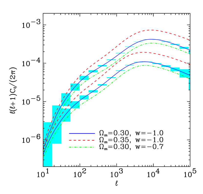
Figure 4: Redshift dependence of the lensing power spectrum. The solid lines and associated $1\sigma$ error boxes show the lensing power spectrum for the two redshift bins of the SNAP wide survey with median galaxy redshifts of $z_{m}=0.96$ (bottom line) and 1.73 (top line). As in figure 2, the dashed and dot-dashed lines correspond to perturbations about the fiducial model (solid line) for each redshift bin.

6 Skewness

Non-linear gravitational instability is known to produce non-gaussian features in the cosmic shear field. The power spectrum therefore does not contain all the information available from weak lensing. We consider the most common measure of non-gaussianity, namely the skewness $S_{3}$ which is defined as (eg. Bernardeau et al. 1997)

$$S_{3}(\theta)\equiv\frac{\langle\kappa^{3}\rangle}{\langle\kappa^{2}\rangle^{2}}$$ (7)

where $\kappa$ is the convergence which can be derived from the shear field $\gamma_{i}$ and the brackets denote averages over circular top-hat cells of radius $\theta$. The denominator is the square of the convergence variance which is given by

$$\langle\kappa^{2}\rangle=\langle\gamma^{2}\rangle\simeq\frac{1}{2\pi}\int d\ell~{}\ell C_{\ell}|W_{\ell}|^{2},$$ (8)

where $W_{\ell}\equiv 2J_{1}(\ell\theta)/(\ell\theta)$ is the window function for such cells and $C_{\ell}$ is the lensing power spectrum given by equation (4).

To evaluate the numerator of equation (7) we use the approximation of Hui (1999) who used the Hyperextended perturbation theory of Scoccimarro & Frieman (1999) and obtained

$$\langle\kappa^{3}\rangle \simeq \frac{81\pi^{2}}{16}\left(\frac{H_{0}}{c}\right)^{6}\Omega_{m}^{3}\times$$ (9)

$$\int_{0}^{\chi_{h}}d\chi~{}\frac{g^{3}}{a^{3}r^{4}}\left[\int d^{2}\ell~{}\sqrt{Q_{3}}P\left(\frac{\ell}{r},\chi\right)|W_{\ell}|^{2}\right]^{2},$$

where $Q_{3}=(4-2^{n})/(1+2^{n+1})$ and $n$ is the linear power spectral index at scale $k=\ell/r$. While more accurate approximations for third order statistics now exist (see van Waerbeke et al. 2001 and reference therein), the present one suffices for our purpose.

Figure 5 shows the skewness as a function of scale for the same cosmological models considered in Figure 2. The skewness is only weakly dependent on the angular scale $\theta$, but depends more strongly on $\Omega_{m}$ and $w$.

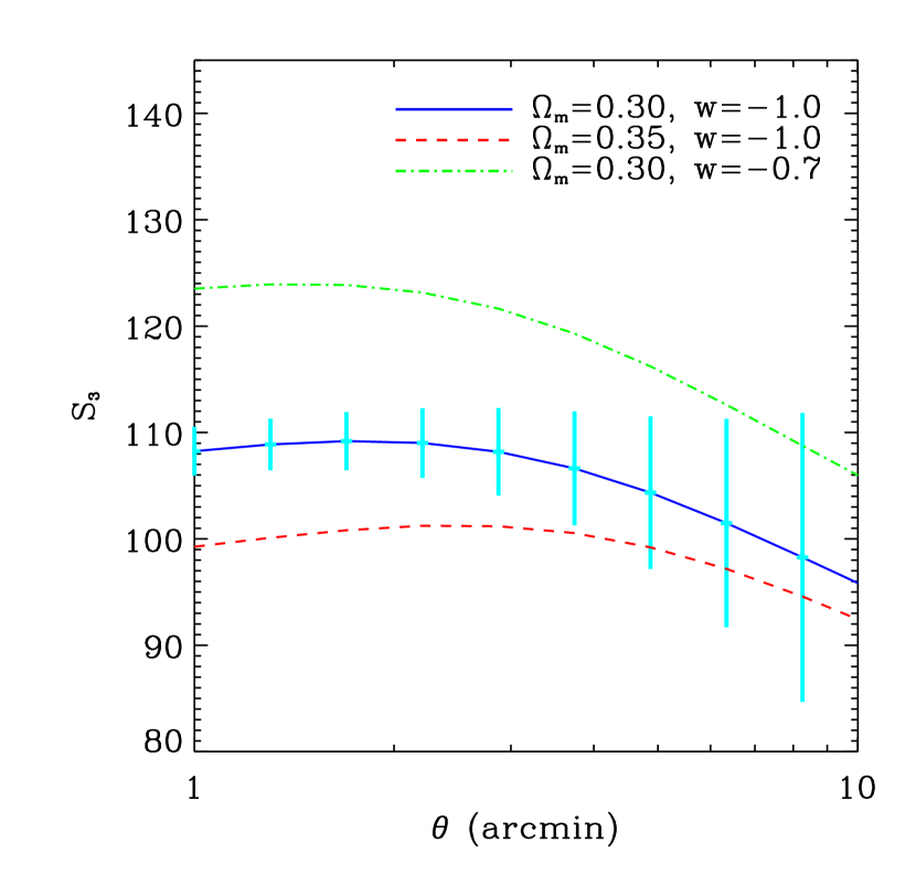
Figure 5: Skewness $S_{3}$ as a function of scale. The three cosmological models from Figure 2 are displayed. The $1\sigma$ error bars correspond to the SNAP wide survey.

The computation of the exact error for $S_{3}$ is challenging as it depends on sixth order terms, which are difficult to compute in the non-linear regime. Instead, we compute the rms error for a gaussian field (in which case $S_{3}=0$) and introduce a multiplicative factor $f_{ng}$ to correct for non-Gaussianity of the convergence field and obtain

$$(\Delta S_{3})^{2}=\frac{15}{N_{c}}\frac{\left[f_{ng}^{\frac{2}{3}}\langle\kappa^{2}\rangle+\sigma_{\kappa}^{2}/(n_{g}A_{c})\right]^{3}}{\langle\kappa^{2}\rangle^{2}},$$ (10)

where $A_{c}=\pi\theta^{2}$ is the cell solid angle, $N_{c}=A/A_{c}$ is the number of cells which are assumed to be independent, and $A$ is the total solid angle of the survey. The rms dispersion of the convergence arising from the intrinsic dispersion of the galaxy ellipticities and from measurement noise is related to the associated rms shear by $\sigma_{\kappa}^{2}=\sigma_{\gamma}^{2}$. The non-gaussian correction factor only applies to the cosmic variance term (first term) since the noise term can be assumed to be gaussian. It is set to $f_{ng}\simeq 2$, as estimated by White & Hu (2000) who compared gaussian estimates with errors derived from (noise-free) numerical simulations.

The resulting errors for SNAP wide survey are shown in Figure 5, for the fiducial $\Lambda$CDM model. The sensitivity afforded by this survey will allow us to easily distinguish between these models via the skewness.

7 Constraints on Cosmological Parameters

7.1 Fisher Matrix

The constraints which can be set on cosmological parameters can be estimated using the Fisher matrix (eg. Hu & Tegmark 1999)

$$F_{ij}=-\left\langle\frac{\partial\ln{\mathcal{L}}}{\partial p_{i}\partial p_{j}}\right\rangle$$ (11)

where ${\mathcal{L}}$ is the Likelihood function, and $p_{i}$ is a set of model parameters. The inverse ${\mathbf{F}}^{-1}$ provides a lower limit for the covariance matrix of the parameters.

For a measurement of the power spectrum this reduces to,

$$F_{ij}=\sum_{\ell}(\Delta C_{\ell})^{-2}\frac{\partial C_{\ell}}{\partial p_{i}}\frac{\partial C_{\ell}}{\partial p_{j}},$$ (12)

where the summation is over modes $\ell$ which can be reliably measured. Note that this expression assumes that the errors are gaussian and that the multipoles are not correlated. These effects have been shown to increase the errors on cosmological parameters by only about 15% (Cooray & Hu 2001) and have been neglected here.

Since the measurement of the skewness on different scales are strongly correlated, we conservatively consider only one scale $\theta=2^{\prime}$ to compute the constraints from $S_{3}$. The associated fisher matrix is then

$$F_{ij}=(\Delta S_{3})^{-2}\frac{\partial^{2}S_{3}}{\partial p_{i}\partial p_{j}}.$$ (13)

The joint constraints from the power spectrum combined with the skewness can be computed by adding the respective Fisher matrices.

7.2 Baseline surveys

Figure 6 shows the joint constraints on $w$ and $\Omega_{m}$ which can be derived from the wide and deep wide surveys. The contours correspond to the 68% confidence level and have been marginalized over $h$, $n$ and $\Omega_{b}$. A COBE prior for the power spectrum normalization $\delta_{h}$ of 7% rms (Bunn & White 1997) was also assumed and marginalized over. The range of scales considered to evaluate the power spectrum is $10<\ell<2\times 10^{5}$.

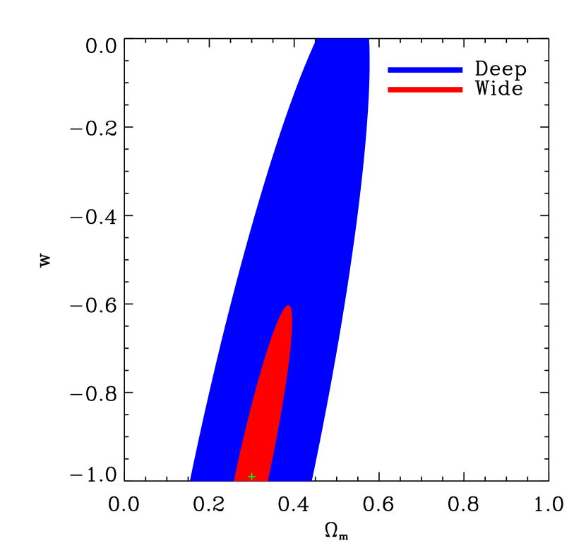
Figure 6: Constraints on $\Omega_{m}$ and $w$ from the power spectrum derived from the wide and deep SNAP surveys. The contours correspond to the 68% confidence level and have been marginalized over $h$, $n$ and $\Omega_{b}$, with a 7% rms COBE prior for the power spectrum normalization $\delta_{h}$. The cosmological model was assumed to be flat ($\Omega_{m}+\Omega_{q}=1$). The range of scales used for the power spectrum is $10<\ell<2\times 10^{5}$.

Clearly, the wide survey provides stronger constraints than the deep survey, even though its observing time is 6.4 times shorter. This follows from the fact that the increased surface density of resolved galaxies in the deep survey does not compensate for its smaller area. This can be seen by comparing the error bars for the power spectrum from each survey (see Figure 3 and the discussion in §3).

7.3 Survey Strategy

It is instructive to study the dependence of these constraints on the survey geometry. Figure 7 shows how the constraints on $\Omega_{m}$ and $w$ change as the survey area $A$ is halved or doubled, while the depth of the survey is kept as that of the wide survey (see parameters for the wide survey in Table 1). As expected, the contours scale simply as $A^{-1/2}$ in this case.

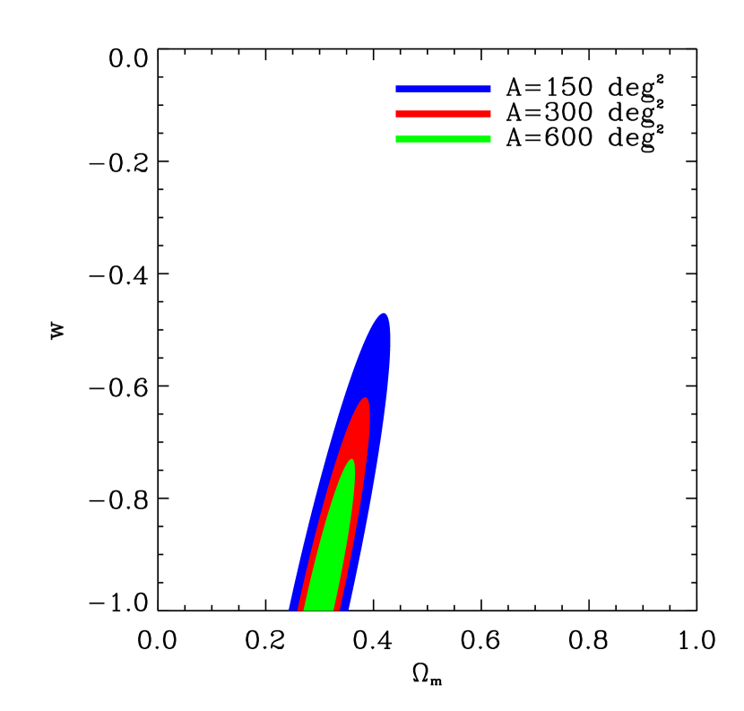
Figure 7: Dependence of the confidence contours on the survey area $A$, for a varying survey observing time $t_{\rm tot}$. The depth of the survey is fixed to that of the wide SNAP survey (300 deg², $t_{\rm tot}=5$ months). A survey area of 150 and 600 deg² would thus require an observing time of 2.5 and 10 months, respectively. The conventions and marginalizations are as described in the caption of Figure 6.

More realistically, Figure 8 shows the same contours, but this time keeping the survey observing time constant to $t_{\rm tot}=5$ months, the allocated time for the wide survey. This amounts to a trade-off between area and depth for a fixed observing time. The survey parameters for each of the 150, 300 and 600 deg² cases are listed in table 1, with entries ‘Wide$-$’, ‘Wide’ and ‘Wide+’, respectively. As can be seen on the figure, the constraints do not improve as fast as in the earlier case. Doubling the survey area from 300 to 600 deg², while reducing the depth correspondingly, leads to an improvement on the precision of $w$ of only about 10%.

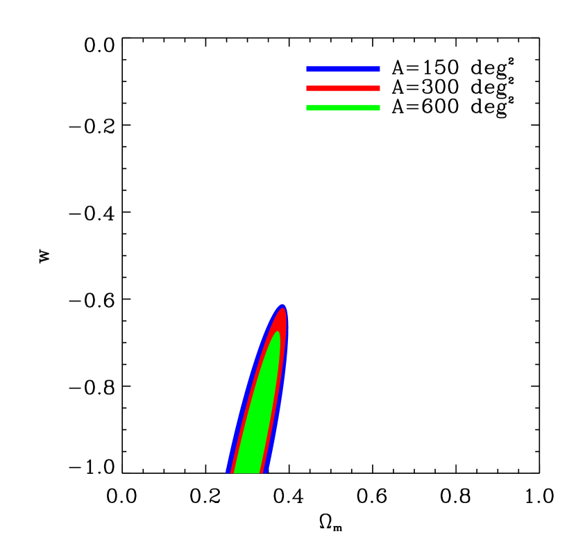
Figure 8: Dependence of the confidence contours on the survey area $A$ for a fixed observing time of $t_{\rm tot}=5$ months. This corresponds to a trade-off between survey width and depth about the nominal SNAP wide survey (300 deg²). The sensitivity to shear for each exposure time was derived from the image simulations described in Paper II.

A wider and shallower survey is therefore preferred compared to the nominal wide survey, but does not provide a substantial improvement. As explained in Paper I, the shallowness of the survey is limited by the finite telemetry bandwidth of the spacecraft, and can not be increased without performing lossy data compression or modification of the hardware. Moreover, a shallower survey will limit our ability to measure the redshift dependence of the lensing power spectrum (see §5.3 and §7.4 below). These considerations led to the choice of the baseline survey strategy of the SNAP wide survey (see Paper I).

7.4 Tomography

As discussed in §5.3, the constraints can be improved by studying the redshift dependence of the lensing power spectrum. This can be done by subdividing the galaxy sample into several redshift bins using photometric redshifts.

Figure 9 shows how the constraints on $w$ and $\Omega_{m}$ improve when the galaxies in the SNAP wide survey are split into 2 and 3 redshift bins. The redshift distribution $n(z)$ of each bin are those in the bottom left panel in Figure 1. The parameters for these distributions are listed in Table 1. The constraints on both $w$ and $\Omega_{m}$ improve by about a factor of 2 in precision when 2 bins are used instead of 1. The gain from additional bins is not very significant. This results agrees with the conclusions of Huterer (2001) and Hu (2001) who considered more generic cases and simpler redshift distributions. Note that our analysis includes the effect of photometric redshift errors and of the resulting leakage from one bin to the other (see overlapping tails in Figure 1).

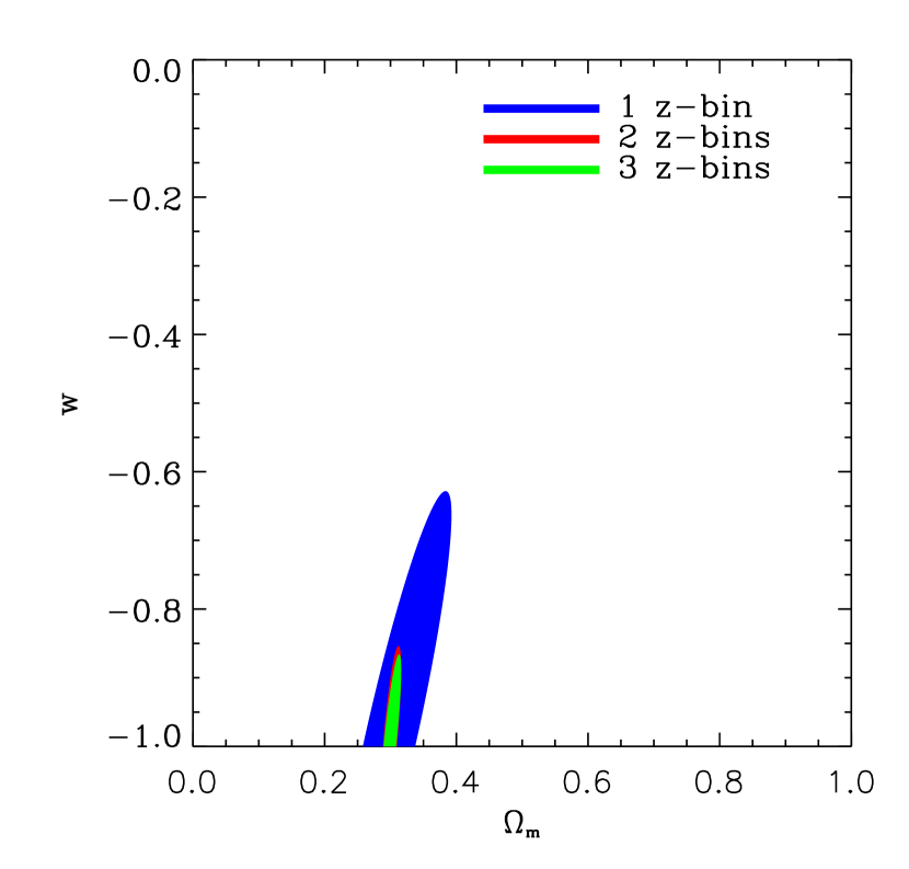
Figure 9: Improvement of the constraints on $w$ and $\Omega_{m}$ from the use of tomography. One, two and three redshift bins derived from photometric redshifts in the SNAP wide survey (with near-IR detectors) are displayed.

7.5 Skewness

As discussed in §6, another way of improving the cosmological constraints is to also include a measurement of the skewness $S_{3}$. Figure 10 shows the contours on the $\Omega_{m}$-$w$ plane corresponding to the use of the power spectrum with and without tomography (with two redshift bins) and with and without skewness. As discussed in §13, a measurement of $S_{3}$ at the single scale of $\theta=2^{\prime}$ is conservatively considered. The addition of the skewness improves the precision on $\Omega_{m}$ by a little less than a factor of 2, but does not appreciably improve the precision of $w$. The former arises from the well known fact that a measurement of $S_{3}$ helps to break the degeneracy between the power spectrum normaliszation and $\Omega_{m}$ (Bernardeau et al. 1997).

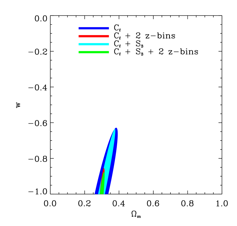
Figure 10: Constraints on $\Omega_{m}$ and $w$ derived from combinations of the power spectrum without tomography ($C_{\ell}$), the power spectrum with 2 redshift bins, and the skewness $S_{3}$. The measurement of $S_{3}$ at the single scale $\theta=2^{\prime}$ is considered.

The improvements on both $\Omega_{m}$ and $w$ from the inclusion of the skewness are however overwhelmed by the corresponding improvements derived from tomography. This shows that tomography is more powerful than the skewness to study dark energy, at least for conditions similar to that of the SNAP wide survey. Note that our treatment of the skewness using the Fisher matrix provides a lower limit for the parameter errors, since the error of the skewness is non-gaussian (this is also true for the power spectrum). This conclusion will thus be a fortiori true for a full non-gaussian treatment of the skewness error. The combined constraints using both tomography and skewness are also displayed in Figure 10.

7.6 Comparison with Constraints from Supernovae

The results described above show that weak lensing provides powerful contraints on dark energy which can be compared with those derived with other methods. Figure 11 compares the constraints from weak lensing to those from supernovae. The filled weak lensing contours include tomography (with 2 redshift bins), the skewness, and the COBE normalization prior. The broad contours correspond to the current constraints from 42 supernovae (Perlmutter et al. 1999). The expected constraints derived from supernovae found in the SNAP deep survey are also shown (Perlmutter et al. 2003). Note that these authors have marginalised over the time derivative $w^{\prime}$ of $w$, and have thus not assumed that $w$ was constant as we have done. In addition, their constraints, unlike ours, include uncertainties due to systematics (see discussion on systematics in §8). As before, all contours correspond to 68% confidence levels.

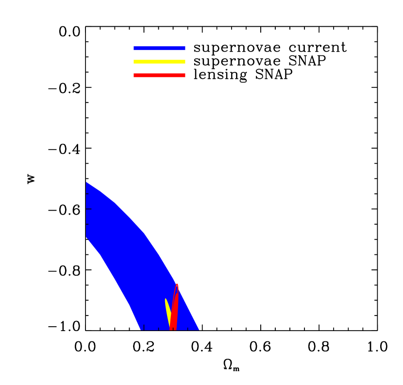
Figure 11: Comparison of the constraints derived from weak lensing and from supernovae. The current constraints from 42 supernovae (Perlmutter et al. 1999) are also displayed, along with those expected from the SNAP deep supernovae survey (Perlmutter et al. 2003). In the latter case, the time derivative $w^{\prime}$ of $w$ was also marginalized over. The weak lensing contours assume the use of 2 redshift bins for the power spectrum and of the skewness. The filled and unfilled contours correspond to the constraints with and without the COBE normalization prior, respectively. As before all contours correspond to 68% confidence levels.

The SNAP weak lensing survey will clearly greatly improve upon the current supernovae constraints on $w$. It will also yield constraints which are comparable and somewhat orthogonal to those derived from the SNAP deep surpernovae survey. Note however that the SNAP weak lensing survey is obtained from 5 months of observations rather than 32 months for the deep supernovae survey.

The unfilled contours in figure 11 show the effect of dropping the COBE prior for the weak lensing constraints. The precision for $\Omega_{m}$ is hardly affected, but that for $w$ is degraded by about 50%. Note that the above conclusions are contingent on the fact that lensing systematic uncertainties are subdominant. This will be discussed in the next section.

8 Conclusions

We have studied the capability of a wide-field space telescope to measure cosmological parameters with weak gravitational lensing. For this purpose, we have used the results of the image simulations described in Paper II to estimate the sensitivity of the lensing shear for several survey strategies, using the SNAP mission as a concrete example. By combining the power spectrum measured in several redshift bins and the skewness of the convergence field, we find that the SNAP wide survey will provide a measure $w$ and $\Omega_{m}$ with a 68%CL uncertainty of approximately 12% and 1.5% respectively. These errors include marginalization over other parameters ($h$, $A$, $n$ and $\Omega_{b}$) using COBE priors for the power spectrum normalization $\delta_{h}$ and assume a flat universe, but neglect systematics (see discussion below). These constraints are comparable and nearly orthogonal to those derived from supernovae in the SNAP deep survey. The constraints on $w$ and $\Omega_{m}$ degrade by a factor of about 2 in the absence of tomography, but are not affected very much if the skewness only is dropped.

We also studied how the constraints on these parameters depend on the survey strategy. We found that, for a fixed observing time of 5 months, they improve slowly if the survey is made wider and shallower. This, combined with the limits imposed by the spacecraft telemetry, confirms the choice of the nominal parameters for the SNAP wide survey.

Note that our analysis relies on a number of assumptions. We first assumed that systematic errors are sub-dominant compared to statistical errors. The level of systematics will be greatly reduced for SNAP, as compared to ground based surveys, thanks to the absence of the atmospheric seeing and due to the stable thermal orbit of the spacecraft. This is confirmed by our assessment of the systematics for the SNAP design described in Paper I. Further instrument and image simulations are however required to confirm these estimates. In addition, the SNAP optical and near-IR filter set will allow us to test and limit the impact of intrinsic galaxy alignements using photometric redshifts (see Heavens 2001 for a review).

We also assumed that the errors for the power spectrum and skewness are gaussian, and thus that the fisher matrix provides good estimates of the errors. We also neglected potential cross talks between the power spectra in different redshift bins. While these effect are not expected to have a large influence on our error estimates (see White & Hu 2000), these approximations ought to be tested in the future using N-body simulations.

Another potential limitation arises from the theoretical uncertainties inherent in the computation of the matter power spectrum and bispectrum (see discussion in Huterer 2001; van Waerbeke et al. 2001). Huterer indeed remarked that significant differences exist between the different available formulae for the non-linear corrections to the matter power spectrum (eg. Peacock & Dodds 1996; Ma et al. 1999) in QCDM models. Larger and more accurate N-body simulations of QCDM models are needed to improve the accuracy of the fitting functions and to establish whether the finite accuracy of the theoretical predictions will be a limitation for the precision reached by future instruments.

Our work demonstrates that weak lensing is a powerful probe of both dark matter and dark energy. The complementarity of the constraints derived from weak lensing and supernovae validates the integration of both techniques in the science goals for SNAP. A joint analysis of the constraints which can be derived from weak lensing, supernovae and CMB anisotropies on both $w$ and its evolution is left to future work.

References

- (1) Bartelmann, M., & Schneider, P. 1999, submitted to Physics Reports, preprint astro-ph/9912508
- (2) Bacon, D.J., Refregier, A., & Ellis, R. 2000, MNRAS, 318, 625
- (3) Bardeen, J.M., Bond, J.R., Kaiser, N., Szalay, A.S., ApJ, 304, 15
- (4) Benabed, K., & Bernardeau, F., 2001, PRD, 64, 083501
- (5) Bernardeau, F., van Waerbeke, L., & Mellier, Y., 1997, A&A, 322, 1
- (6) Bunn, E., & White, M., 1997, ApJ, 480, 6
- (7) Bolzonella, M., Miralles, J.-M., & Pelló, R., 2000 A&A, 363, 476
- (8) Cooray, A., & Hu, W., 2001, ApJ, 554, 56
- (9) Heavens, A., 2001, Procs. Yale Workshop on ‘The Shapes of Galaxies and their halos’, May 2001, Ed. P. Natarajan, preprint astro-ph/0109063
- (10) Hoekstra, H., Yee, H., & Gladders, M., 2002, submitted to NewA Reviews, preprint astro-ph/0205205
- (11) Hu, W., & Tegmark, M., 1999, ApJ, 514, L65
- (12) Hu, W., 1999, ApJ, 522, 21L
- (13) Hu, W., 2001, Phys. Rev. B, 66, 3515
- (14) Hu, W. & Keeton, C.R. 2002, submitted to PRD, preprint astro-ph/0205412
- (15) Huterer, D., 2001, Phys. Rev. D, 65, 6, 063001, preprint astro-ph/0108090
- (16) Hui, L., 1999, ApJ, 519, 9
- (17) Kaiser, N. 1998 ApJ, 498, 26.
- (18) Ma, C.-P., Caldwell, R.R., Bode, P., & Wang, L., 1999, ApJ, 521, L1
- (19) Massey, R. et al., 2003, (Paper II), submitted to ApJ, available on astro-ph
- (20) Mellier, Y., et al., 2002, SPIE Conference 4847 Astronomical Telescopes and Instrumentation, Kona, August 2002, preprint astro-ph/0210091
- (21) Munshi, D., & Wang, Y., 2003, ApJ, 583, 566
- (22) Peacock, J.A., 1997, MNRAS, 284, 885
- (23) Peacock, J.A., & Dodds, 1996, MNRAS, 280, L19
- (24) Perlmutter, S. et al., 2003, SNAP homepage http://snap.lbl.gov
- (25) Perlmutter, S. et al., 1999, ApJ, 517, 565
- (26) Refregier, A., 2003, to appear in ARAA
- (27) Rhodes, J. et al., 2003, (Paper I), submitted to ApJ, available on astro-ph
- (28) Scoccimarro, R., & Frieman, J.A., 1999, ApJ,520,35
- (29) Spergel, D.N., et al. 2003, submitted to ApJ, preprint astro-ph/0302209
- (30) Sugiyama, N. 1995, ApJS, 100, 281
- (31) Taylor, A., 2001, submitted to PRL, preprint astro-ph/0111605
- (32) van Waerbeke, L., et al. 2001, A&A, 374, 757
- (33) van Waerbeke, L., Hamana, T., Soccimarro, R., Colombi, S., Bernardeau, F., 2001, MNRAS, 322, 918
- (34) Weinberg, N.N., & Kamionkowski, M., 2002, submitted to MNRAS, preprint astro-ph/0210134
- (35) White, M., & Hu, W., 2000, ApJ, 537, 1