The intrinsic colour dispersion in Type Ia supernovae

The properties of low-redshift Type Ia supernovae are investigated using published multi-band optical broadband data from the Calan/Tololo and CfA surveys. The average time evolution of $B-V$, $V-R$, $R-I$, $B-I$ and $V-I$, the intrinsic dispersion and time correlations are studied. This information is required to deduce the extinction of such explosions from the measured colours. We find that extinction corrections on individual SNe based on their colours up to 40 days past the ${\mathit{B}}$-band lightcurve maximum are generaly limited to $\sigma_{A_{V}}\raise 1.29167pt\hbox{$>$}\kern-7.5pt{\lower 2.79857pt\hbox{$\sim$}}0.1$, due to intrinsic variations, as far as it can be conservatively deduced with the current sample of data. However, we find that the $V-R$ colour, especially at late times, is consistent with a negligible intrinsic spread, and may be the most accurate estimator for extinction.

1 Introduction

In the last few years Type Ia supernovae (SNe Ia) have proved to be excellent distance estimators and have been successfully used to investigate the fate of the universe (Perlmutter et al., 1999; Riess et al., 1998). Despite the broad use of these objects by cosmologists, the current knowledge of the nature of SNe Ia is rather limited. Thus, there is a strong demand for further understanding to assess important issues about these explosions. For cosmological implications, the main concerns are related to the possible evolution of the SN properties with redshift. Moreover, critical tests for extinction along the line of sight based on supernova colours require good knowledge of the intrinsic properties of these objects.

In this paper, a statistical study on 48 well observed nearby SNe Ia is carried out. In particular, the intrinsic dispersion in SN colours is investigated using published ${\mathit{B}VRI}$ data. We also focus on the time correlation of intrinsic optical colours. This information is needed to address the possible host galaxy or intergalactic extinction by dust of supernovae used for cosmological tests (see e.g. Riess et al. (2000); Nobili et al. (2003)), and also to probe for other exotic sources of dimming at high-z with differential extinction (Mörtsell et al., 2002).

2 The data set

Published ${\mathit{B}VRI}$ lightcurves of well observed nearby SNe Ia were analysed. The considered sample consists of 48 SNe Ia from 2 different sets, the Calan/Tololo data published by Hamuy et al. (1996), and the set in Riess et al. (1999), usually referred to as the CfA data. The list of SNe is given in Table 1, along with the observed filter data available for each of them, their redshift and the ${\mathit{B}}$-band lightcurve “stretch”, s, as defined in Perlmutter et al. (1997) and Goldhaber et al. (2001).
The selected samples include a broad variety of SNe, well distributed in stretch factor, s. This parameter, related to $\Delta m_{\rm 15}$ (Phillips, 1993), has been found to correlate with the supernova luminosity. Thus, a sample well distributed in stretch should imply a broad distribution in luminosity. Fig. 1 shows the distribution of the ${\mathit{B}}$-band light curve stretch factor and SN redshifts ($0.003\leq z\leq 0.12$), for both samples. The timescale stretch parameter was determined from the lightcurve fits as in Goldhaber et al. (2001) using their ${\mathit{B}}$-band lightcurve template with a parabolic behavior for the earliest epoch after explosion.

$K$-corrections were applied to account for the small cosmological redshift as described in e.g. Goobar et al. (2002), using the ($s=1$) spectroscopic template of Nugent et al. (2002) as a starting point. The results of this analysis were used to improve the spectral template of SN Ia’s (Sect. 6) and we iterated the analysis once re-calculating the $K$-corrections with the improved template. Note that even though the $K$-corrections for the used data set are small, typically of the order of a few hundreds of a magnitude, for some of the more distant objects in the sample considered, they reach up to $\sim 0.5$ mag.

The SNe light curves were corrected for both Milky Way and host galaxy extinction as in Phillips et al. (1999) using the method first proposed by Lira (1995) for estimating host galaxy extinction using late epoch light curves. There is empirical evidence that the $B-V$ colors of SNe Ia show extremely small scatter for the period between 30 and 90 days post ${\mathit{B}}$-band maximum, despite any difference in the light curve shapes at earlier epochs. As the set of SNe used in this article is a subset of the one analysed in Phillips et al. (1999), the host galaxy extinctions listed in Table 2 of their paper were used. These were derived combining the late time $B-V$ colour with information on the $B-V$ and $V-I$ at maximum light.

The Cardelli et al. (1989) relation, modified by O’Donnell (1994), was used to compute the extinction in other colours given $E(B-V)$. Spectral templates of Type Ia SNe were used to compute the evolution of the extinction with the supernova epoch.

The extinction corrected lightcurves were further screened to exclude the most peculiar SNe, as the main emphasis of this work is to establish the properties of “normal” supernovae. Fig. 2 shows the difference of the $B$-band lightcurve maximum, $B_{\rm max}$ and the $V$-band light curve maximum $V_{\rm max}$ plotted against the decline rate parameter, $\Delta m_{\rm 15}$, as reported in Phillips et al. (1999). A $3\sigma$ clipping rejection criteria was applied, iterating until no data points were further rejected. At least 5 SNe in the 2 data sets deviate significantly from the expected linear relation derived in Phillips et al. (1999) from an independent set of 20 non-reddened SNe (solid line in Fig. 2):

$$B_{\rm max}-V_{\rm max}=-0.07(\pm 0.012)+0.114(\pm 0.037)(\Delta m_{\rm 15}-1.1)$$

The outliers are SN 1993ae, SN 1995bd, SN 1996ai, and SN 1996bk for the CfA data, and SN 1992K for the Calan/Tololo set. Moreover SN 1995E and SN 1995ac have been excluded since they are similar to the peculiar SN 1991T (Branch et al., 1993).

Table 1: List of SNe used for the analysis.
(1), Riess et al. (1998); (2), Hamuy et al. (1996);
^a excluded from the analysis presented here.

SN	band	$z$	$s$	Ref.
1993ac	B,V,R,I	0.049	0.865	(1)
1993aea	B,V,R,I	0.019	0.846	(1)
1994ae	B,V,R,I	0.004	1.033	(1)
1994M	B,V,R,I	0.023	0.865	(1)
1994Q	B,V,R,I	0.029	1.116	(1)
1994S	B,V,R,I	0.015	1.061	(1)
1994T	B,V,R,I	0.035	0.890	(1)
1995aca	B,V,R,I	0.050	1.123	(1)
1995ak	B,V,R,I	0.023	0.857	(1)
1995al	B,V,R,I	0.005	1.044	(1)
1995bda	B,V,R,I	0.016	1.131	(1)
1995D	B,V,R,I	0.007	1.081	(1)
1995Ea	B,V,R,I	0.012	1.024	(1)
1996aia	B,V,R,I	0.003	1.110	(1)
1996bka	B,V,R,I	0.007	0.761	(1)
1996bl	B,V,R,I	0.036	1.030	(1)
1996bo	B,V,R,I	0.017	0.902	(1)
1996bv	B,V,R,I	0.007	1.106	(1)
1996C	B,V,R,I	0.030	1.102	(1)
1996X	B,V,R,I	0.007	0.889	(1)
1990af	B,V	0.051	0.792	(2)
1990O	B,V,R,I	0.030	1.116	(2)
1990T	B,V,R,I	0.040	0.998	(2)
1990Y	B,V,R,I	0.039	1.007	(2)
1991ag	B,V,R,I	0.014	1.084	(2)
1991S	B,V,R,I	0.055	1.114	(2)
1991U	B,V,R,I	0.032	1.068	(2)
1992ae	B,V	0.075	0.970	(2)
1992ag	B,V,I	0.025	0.951	(2)
1992al	B,V,R,I	0.015	0.963	(2)
1992aq	B,V,I	0.102	0.868	(2)
1992au	B,V,I	0.061	0.787	(2)
1992bc	B,V,R,I	0.020	1.039	(2)
1992bg	B,V,I	0.035	0.983	(2)
1992bh	B,V,I	0.045	1.048	(2)
1992bk	B,V,I	0.058	0.825	(2)
1992bl	B,V,I	0.044	0.812	(2)
1992bo	B,V,R,I	0.019	0.767	(2)
1992bp	B,V,I	0.079	0.907	(2)
1992br	B,V	0.088	0.682	(2)
1992bs	B,V	0.064	1.030	(2)
1992J	B,V,I	0.045	0.798	(2)
1992Ka	B,V,I	0.010	0.787	(2)
1992P	B,V,I	0.037	0.952	(2)
1993ag	B,V,I	0.049	0.917	(2)
1993B	B,V,I	0.070	1.023	(2)
1993H	B,V,R,I	0.024	0.774	(2)
1993O	B,V,I	0.051	0.950	(2)

Figure 1: Distribution of redshift, z, (binsize=0.02), and stretch factor, s, (binsize= 0.08), for the analysed sample

Figure 2: $B_{\rm max}$-$V_{\rm max}$ vs $\Delta m_{\rm 15}$ for the 2 sets of data, k-corrected, corrected for Galactic extinction and Host Galaxy extinction, compared with the result of Phillips et al. (1999)

3 The average optical colours

Figs. 3- 8 show the time evolution of the extinction and $K$-corrected $B-V$, $V-R$, $R-I$, $B-I$ and $V-I$, colours. The plotted errors include the uncertainty on the host galaxy exinction correction. The time axis ($t^{\prime}$) has been corrected by the SN redshift and the ${\mathit{B}}$-band stretch factor $s$, to account for the dependence of colours on the stretch. This rescaling of the time axis was found very effective in reducing the measured intrinsic dispersion (Sect. 4)

$${t^{\prime}}={t-t_{B_{\rm max}}\over s\cdot(1+z)}$$ (1)

For each colour lightcurve we have spline-interpolated the weighted mean values computed in four days wide, non-overlapping bins. The aim of this procedure was to find a curve that describes the average time evolution of the colours. This parameterization will be referred as a “model” in the following discussion. Other methods were used to fit the data, as for example a least squares cubic spline fit. These result in curves that differ from the model typically by 0.01 magnitudes. The models show some systematic discrepancies between the two data sets, especially in $R-I$ for which the C-T model is always redder than the CfA model. In Fig.  9 we investigate the differences of each of the models from the one built on both sets together. The differences are usually of the order of a few hundreds of a magnitude. The largest deviation was found for $R-I$ in the Calan/Tololo set, resulting in a difference of about 0.2 mag at maximum with respect to the model built up using data from both sets. Note, however, that the statistics in the Calan/Tololo set for $R-I$ colour, all along the evolution and in particular around the time of $B_{\rm max}$, is extremely poor, as shown in Fig. 5. Due to the smaller quoted observational error bars, the CfA set dominates the weighted average used to build the model out of both data sets.

A source of uncertainty in this analysis is the ability of the observers to convert the instrumental magnitudes from the used filter+CCD system transmission into the standard ${\mathit{B}VRI}$ system. The apparent systematic effects for $R-I$ in Fig. 9 may be indicative of this.

Figure 3: $B-V$ for the two sets of data. The solid line represent alway the curve found for the current set, while the dashed line is the curve found for the same colour of the other set.

Figure 4: $V-R$ for the two sets of data. The solid line represent alway the curve found for the current set, while the dashed line is the curve found for the same colour of the other set.

Figure 5: $R-I$ for the two sets of data. The solid line represent alway the curve found for the current set, while the dashed line is the curve found for the same colour of the other set.

Figure 6: $B-I$ for the two sets of data. The solid line represent alway the curve found for the current set, while the dashed line is the curve found for the same colour of the other set. The filled circles represent SN 1993H, while the filled diamonds are data of SN 1992bc. Refer to Sect. 7 for a discussion about these 2 SNe.

In order to assess systematic effects in builing the colour models, we checked whether the host galaxy extinction was over-corrected. Thus, we compared the models with the data of those SNe that, according to Phillips et al. (1999), suffered no extinction from the host galaxy. The comparison, shown in Fig. 7, exhibits no obvious deviations and we may conclude that the extinction corrected colours are consistent with the uncorrected sub-sample.

A possible remaining dependence of colours on the stretch factor $s$ was investigated. For data points in a 5 days broad bin around time of B-maximum and around day 15, a linear weighted fit was done on the residuals from the models not showing any further significant dependence on $\Delta m_{\rm 15}$ or equivalently on the stretch parameter $s$. Note that this is not in contradiction with Fig. 2, as we are considering $(B-V)_{t_{B_{\rm max}}}$ instead of $B_{\rm max}-V_{\rm max}$. Moreover, our analysis includes data points in a broad bin around day zero, and not a fitted lightcurve maximum as in Fig. 2.

Figure 7: Comparison of the models with data of unreddened SNe only.

Figure 8: V-I for the two sets of data. The solid line represent alway the curve found for the current set, while the dashed line is the curve found for the same colour of the other set. The filled circles represent SN 1993H, while the filled diamonds are data of SN 1992bc. Refer to Sect. 7 for a discussion about these 2 SNe.

Figure 9: Residuals of each of the models from the one built for all the data set.

4 Intrinsic colour dispersion

The observed colour dispersion around the models is overall inconsistent with a statistical random distribution of the data with the reported measurement errors. The $\chi^{2}$ value per degree of freedom computed for each model is typically between 3 and 6, giving indication of a very poor fit of the data. Thus, we conclude that the analysed data supports the existence of an intrinsic colour dispersion of Type Ia supernovae .

The intrinsic colour dispersion was computed on the residuals of each of the data sets from the corresponding model, built as explained above. Labeling $XY_{i}$ any of the measured colours, $B-V$, $V-R$, $R-I$, $B-I$ and $V-I$, the residual with respect to the model expectation is referred as $R_{{XY}_{i}}$, i.e.,

$$R_{{XY}_{i}}={XY}_{i}-XY^{\rm model}_{i}$$ (2)

Next, the time axis was binned into 5 days wide bins to compensate for the modest statistics. The bins are centered at days $d=5\cdot n$, with $n$ ranging from 0 to 8. For each bin $k$, we compute the weighted average for the data ${XY}$, (see Appendix A)

$$XY^{k}=\frac{\sum_{i=1}^{N_{k}}w_{i}XY_{i}}{\sum_{i=1}^{N_{k}}w_{i}}$$ (3)

where $N_{k}$ is the number of points in bin $k$ and $w_{i}$ is the inverse of the uncertainty on the $i$-th measurement squared, $1/\sigma_{i}^{2}$, where $\sigma_{i}$ include both measurement errors and uncertainty on the host galaxy extinction corrections. The weighted sample standard deviation was computed as the square root of the weighted second moment:

$$s_{XY}^{k}=\sqrt{m_{w_{2}}}=\sqrt{\frac{\sum_{i=1}^{N}w_{i}R_{{XY}_{i}}^{2}}{\sum_{i=1}^{N}{w_{i}}}}$$ (4)

The uncertainty on the expression in Eq. (4) is given by the square root of the variance, $V[s_{XY}^{k}]$, computed as:

$$V[s_{XY}^{k}]=\frac{V[m_{w_{2}}]}{4m_{w_{2}}}$$ (5)

Table 2: Results of the analysis of all SNe. First column: central value in days for each time bin; $N_{k}$ is the number of points for each bin; $XY^{k}$ is the weighted mean value and its 1-sigma uncertainty; $\Delta_{XY}$ is the intrinsic dispersion computed according to Eqs. (4) and (5); $\Delta_{XY}^{\rm corr}$ is the corrected intrinsic dispersion, computed as in Eq. (6), and in the last column is the estimated lower limit at 99% C.L. (see text);
^a compatible with null intrinsic dispersion at 99% C.L.; an upper limit is given instead of the corrected intrinsic dispersion.

day	$N_{k}$	$BV^{k}$	$\Delta_{BV}$	$\Delta_{BV}^{\rm corr}$	L.L.
0	57	-0.11 $\pm$ 0.01	0.09 $\pm$ 0.01	0.07	0.05
5	70	0.02 $\pm$ 0.01	0.10 $\pm$ 0.01	0.08	0.05
10	75	0.16 $\pm$ 0.01	0.11 $\pm$ 0.01	0.09	0.06
15	59	0.47 $\pm$ 0.02	0.11 $\pm$ 0.01	0.09	0.06
20	47	0.75 $\pm$ 0.03	0.13 $\pm$ 0.02	0.11	0.08
25	39	0.95 $\pm$ 0.02	0.10 $\pm$ 0.02	0.08	0.06
30	34	1.08 $\pm$ 0.02	0.11 $\pm$ 0.02	0.09	0.07
35a	27	1.07 $\pm$ 0.02	0.08 $\pm$ 0.03	$<$ 0.05
40	35	1.02 $\pm$ 0.02	0.10 $\pm$ 0.03	0.07	0.06
day	$N_{k}$	$VR^{k}$	$\Delta_{VR}$	$\Delta_{VR}^{\rm corr}$	L.L.
0	31	0.04 $\pm$ 0.02	0.07 $\pm$ 0.01	0.06	0.05
5	36	-0.01 $\pm$ 0.02	0.08 $\pm$ 0.01	0.06	0.05
10	38	-0.08 $\pm$ 0.01	0.06 $\pm$ 0.01	0.04	0.04
15	34	-0.07 $\pm$ 0.02	0.07 $\pm$ 0.02	0.06	0.05
20	24	0.09 $\pm$ 0.02	0.06 $\pm$ 0.02	0.05	0.04
25a	22	0.22 $\pm$ 0.02	0.06 $\pm$ 0.01	$<$ 0.04
30a	18	0.31 $\pm$ 0.01	0.06 $\pm$ 0.01	$<$ 0.04
35a	16	0.30 $\pm$ 0.01	0.04 $\pm$ 0.01	$<$ 0.03
40a	19	0.25 $\pm$ 0.01	0.05 $\pm$ 0.01	$<$ 0.03
day	$N_{k}$	$RI^{k}$	$\Delta_{RI}$	$\Delta_{RI}^{\rm corr}$	L.L.
0	30	-0.44 $\pm$ 0.02	0.10 $\pm$ 0.01	0.09	0.06
5	36	-0.50 $\pm$ 0.02	0.09 $\pm$ 0.01	0.07	0.05
10	32	-0.50 $\pm$ 0.02	0.07 $\pm$ 0.01	0.05	0.05
15	30	-0.25 $\pm$ 0.04	0.12 $\pm$ 0.03	0.11	0.08
20	20	-0.06 $\pm$ 0.04	0.13 $\pm$ 0.02	0.12	0.09
25	22	0.09 $\pm$ 0.02	0.08 $\pm$ 0.01	0.05	0.05
30	18	0.23 $\pm$ 0.03	0.08 $\pm$ 0.01	0.06	0.06
35a	16	0.27 $\pm$ 0.03	0.09 $\pm$ 0.01	$<$ 0.06
40	17	0.22 $\pm$ 0.04	0.14 $\pm$ 0.03	0.13	0.10
day	$N_{k}$	$BI^{k}$	$\Delta_{BI}$	$\Delta_{BI}^{\rm corr}$	L.L.
0	39	-0.54 $\pm$ 0.02	0.13 $\pm$ 0.01	0.10	0.08
5	48	-0.52 $\pm$ 0.02	0.15 $\pm$ 0.02	0.13	0.09
10	48	-0.44 $\pm$ 0.03	0.17 $\pm$ 0.01	0.15	0.10
15	35	0.10 $\pm$ 0.05	0.18 $\pm$ 0.02	0.16	0.11
20	34	0.74 $\pm$ 0.06	0.24 $\pm$ 0.05	0.23	0.15
25	25	1.25 $\pm$ 0.05	0.22 $\pm$ 0.04	0.21	0.15
30	27	1.66 $\pm$ 0.03	0.16 $\pm$ 0.02	0.13	0.10
35a	23	1.65 $\pm$ 0.03	0.12 $\pm$ 0.02	$<$ 0.08
40	33	1.51 $\pm$ 0.04	0.20 $\pm$ 0.02	0.17	0.13
day	$N_{k}$	$VI^{k}$	$\Delta_{VI}$	$\Delta_{VI}^{\rm corr}$	L.L.
0	37	-0.43 $\pm$ 0.02	0.08 $\pm$ 0.01	0.05	0.05
5	51	-0.54 $\pm$ 0.02	0.11 $\pm$ 0.01	0.09	0.06
10	48	-0.60 $\pm$ 0.01	0.09 $\pm$ 0.01	0.06	0.05
15	38	-0.34 $\pm$ 0.03	0.13 $\pm$ 0.02	0.11	0.08
20	36	0.01 $\pm$ 0.03	0.14 $\pm$ 0.02	0.13	0.09
25	28	0.33 $\pm$ 0.03	0.15 $\pm$ 0.02	0.14	0.10
30	28	0.57 $\pm$ 0.03	0.12 $\pm$ 0.02	0.10	0.08
35	25	0.58 $\pm$ 0.02	0.10 $\pm$ 0.01	0.08	0.07
40	33	0.48 $\pm$ 0.03	0.13 $\pm$ 0.01	0.11	0.08

where $V[m_{w_{2}}]$ is the variance of the weighted second moment. We can consider the result of Eq. (4) as an estimate of the intrinsic dispersion in each bin, for each $XY$ colour: $\Delta_{XY}=s_{XY}^{k}$. This has been applied at each one of the sets separately and at the whole set of data. The results of the method for the whole set of data are given in Table 2.

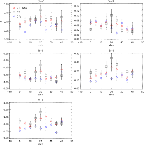
Figure 10: Comparison of the results for the intrinsic dispersion in each colour given in Table 2 for both data sets (triangles) and the results obtained keeping the 2 sets of data separated (squares and diamonds for the C-T and CfA respectively)

Fig. 10 shows a comparison of the intrinsic dispersion computed for each of the sets separately and their combination. In most of the cases the differences exceed the statistical uncertainties, seemingly arising from systematic differences between the two data sets. The computed intrinsic dispersion for the CfA sample was found to be smaller than for the CT data set and the whole (combined) sample in most cases, again pointing at systematic differences in the reported magnitudes.

Note that the adopted method leads to an overestimation of the intrinsic colour dispersion due to the contribution from the measurement errors. However, the weighting procedure ensures that the most accurate measurements dominate the result. To asses the impact of the measurement accuracy, we run a Monte-Carlo simulation to generate a synthetic colour data set with a dispersion given by the measurement uncertainties alone, i.e. no intrinsic dispersion. Three hundred data sets, with the same distributions in epochs and formal error bars as the CfA and Calan/Tololo were simulated and the weighted standard deviation (and its error) were computed, according to Eqs. (4) and (5). Note that the simulation, for simplicity, generates gaussian distributed and completely uncorrelated data. The averages, $\delta$, were used to disentangle the contribution of the intrinsic dispersion from the measurement errors. First, an hypothesis test was run to verify whether the simulated data and the measured data had the same dispersion; e.g. implying null intrinsic dispersion:

$H_{0}:\Delta=\delta$

$H_{1}:\Delta\neq\delta$

A level of significance $\alpha=0.01$ was set for rejecting the null hypothesis, (Cowan, 1998). Only 10 cases were not rejected, indicated by a ^(a) in Table 2. For all the other cases, for which the $H_{0}$ hypothesis was rejected, the intrinsic dispersion was computed as:

$$\Delta^{\rm corr}=\sqrt{\Delta^{2}-\delta^{2}}\\$$ (6)

and a lower limit on its value was set at a 99% confidence limit. The cases for which the null hypothesis was not rejected, were considered as compatible with no intrisic dispersion, and an upper limit on its value was set at a 99% confidence level. The corrected intrinsic dispersions are listed in the 5:th column of Table  2, together with upper and lower limits. We notice that the narrowest colour dispersion happens for $V-R$, especially at late times. At 25 days after $B_{\rm max}$ and later, this colour is compatible with no intrinsic spread at all. Further, it should be noted that at day 35, all the colours but $V-I$ are consistent with vanishing intrinsic dispersion.

5 Correlation

The correlation between optical colours at different epochs was also estimated. The property that was tested is whether a supernova that is blue at a certain epoch for example, say at maximum, stays blue at all epochs. In Riess et al. (2000), the authors argue that data measurements more than 3 days apart may be considered as uncorrelated estimators of colour. Our analysis does not support that assumption. We find significant correlations for data points up to a month apart, as shown below. The method followed is essentially the one used to compute the intrinsic dispersion. One can summarize the following steps:

• Bin the data in time

• Select only the SNe present in all the time bins

• For each bin compute the weighted average of the measurements belonging to the same SN.

• Compute the linear correlation coefficient between bins as in equation A-8.

• Test the correlation coefficient significance (Appendix A.2)

We refer to appendix A.2 for what follows. The correlation coefficient between different epochs h and k is:

$$r_{hk}=\frac{\sum_{i=1}^{n}(R_{XY_{i}}^{h}-\overline{R}_{XY}^{h})(R_{XY_{i}}^{k}-\overline{R}_{XY}^{k})}{\sqrt{\sum_{i=1}^{n}(R_{XY_{i}}^{h}-\overline{R}_{XY}^{h})^{2}\sum_{j=1}^{n}(R_{XY_{j}}^{k}-\overline{R}_{XY}^{k})^{2}}}$$ (7)

where the summation is on the i-th SN, which by construction is present in all the bins. The uncertainty on $r_{hk}$ has been computed converting it into the normally distributed variable z, as described in (Appendix  A.2). The results, given in Table 3, show that the correlation is important and non-zero all along the time evolution. Fig. 11 shows the weighted mean colours for the selected SNe in the bins centered at day 0, 15 and 30. Note that the supernovae selected are different in different colours, but, by construction, are the same in all the bins for each of the colour. It appears that supernovae that deviate from the average colour at a certain epoch are likely to keep their colour excess all along the 30 days evolution considered here.

Table 3: Correlation coefficients between the different bins. The indicated xbin is the central value of each bin. The bin size is 7 days for all the bins. The errors indicate the 1 $\sigma$ confidence level for the computed coefficients. See text for details.

$B-V$/xbin	0	7	15	22	30
0	1.00	$0.80_{-0.14}^{+0.09}$	$0.61_{-0.24}^{+0.16}$	$0.47_{-0.28}^{+0.21}$	$0.45_{-0.28}^{+0.21}$
7		$1.00$	$0.75_{-0.17}^{+0.11}$	$0.69_{-0.20}^{+0.13}$	$0.63_{-0.23}^{+0.15}$
15			$1.00$	$0.59_{-0.24}^{+0.17}$	$0.45_{-0.28}^{+0.22}$
22				$1.00$	$0.56_{-0.25}^{+0.18}$
30					$1.00$
$V-R$/xbin	0	7	15	22	30
0	$1.00$	$0.81_{-0.31}^{+0.13}$	$0.46_{-0.54}^{+0.33}$	$0.29_{-0.56}^{+0.41}$	$0.03_{-0.53}^{+0.51}$
7		$1.00$	$0.24_{-0.56}^{+0.44}$	$0.48_{-0.53}^{+0.32}$	$0.24_{-0.56}^{+0.44}$
15			$1.00$	$0.48_{-0.53}^{+0.32}$	$-0.15_{-0.47}^{+0.55}$
22				$1.00$	$-0.44_{-0.34}^{+0.55}$
30					$1.00$
$R-I$/xbin	0	7	15	22	30
0	$1.00$	$0.73_{-0.51}^{+0.20}$	$0.57_{-0.63}^{+0.31}$	$0.56_{-0.63}^{+0.31}$	$0.31_{-0.68}^{+0.46}$
7		$1.00$	$0.66_{-0.57}^{+0.25}$	$0.78_{-0.45}^{+0.16}$	$0.58_{-0.63}^{+0.30}$
15			$1.00$	$0.89_{-0.28}^{+0.08}$	$0.53_{-0.65}^{+0.33}$
22				$1.00$	$0.83_{-0.38}^{+0.13}$
30					$1.00$
$V-I$/xbin	0	7	15	22	30
0	$1.00$	$0.84_{-0.17}^{+0.08}$	$0.92_{-0.09}^{+0.04}$	$0.93_{-0.08}^{+0.04}$	$0.49_{-0.36}^{+0.25}$
7		$1.00$	$0.72_{-0.26}^{+0.15}$	$0.74_{-0.25}^{+0.14}$	$0.50_{-0.36}^{+0.24}$
15			$1.00$	$0.90_{-0.12}^{+0.06}$	$0.49_{-0.36}^{+0.25}$
22				$1.00$	$0.65_{-0.30}^{+0.18}$
30					$1.00$
$B-I$/xbin	0	7	15	22	30
0	$1.00$	$0.62_{-0.35}^{+0.20}$	$0.74_{-0.27}^{+0.14}$	$0.44_{-0.42}^{+0.29}$	$0.30_{-0.44}^{+0.34}$
7		$1.00$	$0.76_{-0.26}^{+0.13}$	$0.47_{-0.41}^{+0.27}$	$0.51_{-0.39}^{+0.25}$
15			$1.00$	$0.76_{-0.26}^{+0.14}$	$0.40_{-0.42}^{+0.30}$
22				$1.00$	$0.73_{-0.28}^{+0.15}$
30					$1.00$

Figure 11: From top to bottom and left to right. Residuals from the models for the SNe selected for each colour, in bin centered at day 0,15 and 30. The band defined by the solid lines correspond to the intrinsic dispersion found in at the same epoch.

6 Supernovae template

Nugent et al. (2002) analysed the relation between colours of SNe Ia and $K$-corrections. In particular they showed how $K$-corrections are mainly driven by the overall colour of the SN rather than by peculiarities of single features. Using spectra and colour light curves they give a recipe to build a SN Ia template, to be used for computing $K$-corrections of $s\sim 1.0$ SNe. As the sample used in our work is larger than the one considered in their paper, we have used our results to improve the spectral template. Note that this affects only the ${\mathit{B}VRI}$ magnitudes, which are the only bands treated here. Referring to Nugent et al. (2002), we proceed as follows:

• correct the ${\mathit{B}VRI}$ of their list of ${\mathit{U}BVRIJHK}$ magnitudes using our $B-V$, $V-R$ and $R-I$ models

• correct the corresponding spectral templates with this colours

• iterate the whole analysis described in this paper, using the newly created templates to compute the $K$-corrections for both Calan/Tololo and CfA data set

• correct again the templates using the most recent version of the models

Even though the template itself is modified considerably from the original one, iterating once results in small corrections ($\sim$ 0.001-0.005 mag) in the intrinsic dispersion in all colours at any epoch, and a few percent in the colour models. As the correction obtained are small and well within the given uncertainties, we do not iterate further. The results of this analysis should not be considered definitive and may change as SNe Ia and their colour evolutions are studied in even more detail. However, it can be considered a good estimate of the average SN Ia template (in ${\mathit{B}VRI}$), as it is constructed from a quite broad sample of SNe. The final corrected template is available upon request.

7 Discussion

Throughout our analysis all data points were treated as independent measurements. This is particularly important for the cases with significant host galaxy light underneath the supernova where a single reference image was used, introducing a correlation between the data points not considered here.

A first estimate of the intrinsic dispersion was calculated for each data set separately and the two data sets together. A comparison of the results shows that the colours extracted from the CfA sample have smaller scatter indicating that the contribution from measurement errors is not negligible. Further, in the analysis the measurements are assumed to be Gaussian distributed and the weighted standard deviation has been taken as an estimate of the intrinsic dispersion. However, we noticed that 2 SNe, SN 1993H and SN 1992bc, seem to be rather deviant in $B-I$ and $V-I$ for the C-T set, as shown in Figs.  6 and  8. The effect of the “outliers” is particularly important aroud 20 days after B-maximum. For comparison, we recalculated the intrinsic spread in $B-I$ and $V-I$ excluding these 2 SNe. The results are shown on Table 4. The agreement between the intrinsic dispersion between the data sets improves when these 2 SNe are excluded. We emphasize that there are systematic differences between the Calan/Tololo and CfA data sets, and they might have been introduced while converting from the instrumental system used to the standard ${\mathit{B}VRI}$ system.

An attempt of disentangling the intrinsic dispersion from the contribution of the uncertainties has been done resulting in upper limit values for the intrinsic dispersion in some cases. The most relevant is the case of $V-R$, that seems compatible with null intrinsic dispersion for most of the epochs at 99% C.L. Moreover this analysis brings out an important feature at day 35, when all the colours but $V-I$ are consistent with zero intrinsic dispersion. This indicates that further studies will be needed to investigate this intriguing finding.

Table 4: Results of the analysis done excluding SN 1992bc and SN 1993H (**) for $B-I$ and $V-I$. xbin is the central value in days for each bin; $XY^{k}$** is the weighted mean value and its uncertainty; $\Delta_{BI}$** is computed according to Eqs. (4) and (5); $\Delta_{XY}^{\rm corr}$** is the corrected intrinsic disperion and L.L is the lower limit at 99% C.L.; In the last column is the difference between the results given in Table  2 and this analysis; the errors are computed as sum in quadrature.

day	$BI^{k}$**	$\Delta_{BI}$**	$\Delta_{BI}^{\rm corr}$**	L.L.	$\Delta_{BI}-\Delta_{BI}$**
0	-0.53 $\pm$ 0.02	0.13 $\pm$ 0.01	0.10	0.08	0.000 $\pm$ 0.017
5	-0.53 $\pm$ 0.02	0.13 $\pm$ 0.01	0.10	0.08	0.024 $\pm$ 0.025
10	-0.41 $\pm$ 0.02	0.15 $\pm$ 0.02	0.13	0.09	0.018 $\pm$ 0.022
15	0.10 $\pm$ 0.05	0.18 $\pm$ 0.02	0.16	0.11	0.003 $\pm$ 0.026
20	0.74 $\pm$ 0.05	0.15 $\pm$ 0.02	0.12	0.09	0.098 $\pm$ 0.052
25	1.31 $\pm$ 0.05	0.12 $\pm$ 0.02	0.09	0.08	0.101 $\pm$ 0.044
30	1.68 $\pm$ 0.03	0.12 $\pm$ 0.02	0.08	0.08	0.038 $\pm$ 0.028
35	1.65 $\pm$ 0.03	0.13 $\pm$ 0.02	$<$ 0.09		-0.006 $\pm$ 0.024
40	1.49 $\pm$ 0.04	0.20 $\pm$ 0.03	0.18	0.13	-0.004 $\pm$ 0.035
day	$VI^{k}$**	$\Delta_{VI}$**	$\Delta_{VI}^{\rm corr}$**	L.L.	$\Delta_{VI}-\Delta_{VI}$**
0	-0.43 $\pm$ 0.02	0.07 $\pm$ 0.01	0.05	0.05	0.002 $\pm$ 0.011
5	-0.55 $\pm$ 0.01	0.09 $\pm$ 0.01	0.06	0.05	0.019 $\pm$ 0.014
10	-0.58 $\pm$ 0.01	0.09 $\pm$ 0.01	0.06	0.05	0.002 $\pm$ 0.013
15	-0.34 $\pm$ 0.03	0.11 $\pm$ 0.01	0.09	0.07	0.016 $\pm$ 0.022
20	0.01 $\pm$ 0.03	0.11 $\pm$ 0.02	0.09	0.07	0.036 $\pm$ 0.027
25	0.35 $\pm$ 0.03	0.09 $\pm$ 0.01	0.07	0.06	0.060 $\pm$ 0.028
30	0.57 $\pm$ 0.03	0.11 $\pm$ 0.02	0.09	0.07	0.007 $\pm$ 0.029
35	0.58 $\pm$ 0.02	0.10 $\pm$ 0.01	0.08	0.07	0.000 $\pm$ 0.019
40	0.47 $\pm$ 0.03	0.13 $\pm$ 0.01	0.11	0.08	0.000 $\pm$ 0.018

When computing the correlation coefficients we considered data up to 30 days after ${\mathit{B}}$-band maximum, even though later epoch data are available for several supernovae. However, the necessary condition of each SN being observed in all the time bins reduces the statistics if later epochs are introduced. This limitation is specific to the sample used and can be overcome with the use of a more extensively observed sample, such as what will be provide by SNfactory (Aldering et al., 2002).

The intrinsic dispersion sets constrains on the ability to determine the host galaxy extinction,$A_{V}$. This will depend on the colour, as the intrinsic dispersion is different for different colours. As an example we used the Cardelli et al. (1989) relation at the effective wavelength for each bandpass to compute the expected uncertainty in the extinction, neglecting any dependence on the supernova phase.

$$\begin{array}[]{lll}\sigma_{A_{V}}^{\rm B-V}&=&3.1\cdot\Delta_{\rm BV}^{\rm corr}\\ \sigma_{A_{V}}^{\rm V-R}&=&6.2\cdot\Delta_{\rm VR}^{\rm corr}\\ \sigma_{A_{V}}^{\rm R-I}&=&4.1\cdot\Delta_{\rm RI}^{\rm corr}\\ \sigma_{A_{V}}^{\rm B-I}&=&1.4\cdot\Delta_{\rm BI}^{\rm corr}\\ \sigma_{A_{V}}^{\rm V-I}&=&2.5\cdot\Delta_{\rm VI}^{\rm corr}\\ \end{array}$$ (8)

where $R_{V}$ was assumed equal to 3.1. Table 5 shows the results of the equation 8 for the epochs for which the intrinsic dispersion was calculated. The $\Delta_{XY}^{\rm corr}$ was used for this. The results indicate that, with the present knowledge, extinction by dust with $R_{V}=3.1$ may only be determined to $\sigma_{A_{V}}\raise 1.29167pt\hbox{$>$}\kern-7.5pt{\lower 2.79857pt\hbox{$\sim$}}0.10$ with Type Ia restframe optical data within the first 40 days after ${\mathit{B}}$-band lightcurve maximum, for the colours and epochs with non-zero intrinsic dispersion. However observations in $V-R$ are preferable to other colours to set limit on the extinction of an observed supernova. To account for possible different extinction parameters $R_{V}$ in the different supernova host galaxies (as noticed in e.g. (Riess et al., 1996) and (Krisciunas et al., 2000)), we repeated the analysis considering a Gaussian uncertainty $\sigma_{R_{V}}=1$ on $R_{V}$, propagating this scatter on the host galaxy extinction corrections. This changes the values of the intrinsic dispersion, but typically within the quoted errors in Table 2.

Table 5: $\sigma_{A_{V}}$ represent the constrain on the extinction $A_{V}$ that it is possible to compute for a given intrinsic dispersion. The $\Delta_{XY}^{\rm corr}$ and it L.L given in Table 2 has been used for these estimates.

	xbin	$\sigma_{A_{V}}$	L.L.
$B-V$	0	0.23	0.16
$B-V$	5	0.25	0.17
$B-V$	10	0.28	0.18
$B-V$	15	0.28	0.20
$B-V$	20	0.34	0.24
$B-V$	25	0.25	0.20
$B-V$	30	0.27	0.22
$B-V$	35	$<$ 0.16
$B-V$	40	0.21	0.20
$V-R$	0	0.36	0.28
$V-R$	5	0.38	0.29
$V-R$	10	0.27	0.22
$V-R$	15	0.36	0.29
$V-R$	20	0.29	0.26
$V-R$	25	$<$ 0.27
$V-R$	30	$<$ 0.25
$V-R$	35	$<$ 0.19
$V-R$	40	$<$ 0.20
$R-I$	0	0.37	0.27
$R-I$	5	0.28	0.22
$R-I$	10	0.22	0.19
$R-I$	15	0.46	0.32
$R-I$	20	0.48	0.36
$R-I$	25	0.22	0.21
$R-I$	30	0.25	0.23
$R-I$	35	$<$ 0.25
$R-I$	40	0.54	0.41
$V-I$	0	0.12	0.12
$V-I$	5	0.22	0.16
$V-I$	10	0.16	0.13
$V-I$	15	0.27	0.20
$V-I$	20	0.32	0.22
$V-I$	25	0.35	0.25
$V-I$	30	0.25	0.19
$V-I$	35	0.19	0.17
$V-I$	40	0.26	0.20
$B-I$	0	0.14	0.11
$B-I$	5	0.18	0.13
$B-I$	10	0.20	0.14
$B-I$	15	0.22	0.16
$B-I$	20	0.32	0.21
$B-I$	25	0.29	0.21
$B-I$	30	0.18	0.14
$B-I$	35	$<$ 0.12
$B-I$	40	0.24	0.18

8 Conclusion

A statistical analysis of colours of SNe Ia using a sample of 48 nearby SNe was performed. Of this sample 7 SNe have been excluded based on their large extinction, or peculiar behavior of their colours at maximum. With the present knowledge and data quality we computed the average colour evolution for $B-V$, $V-R$, $R-I$, $B-I$ and $V-I$ with time and the derived intrinsic scatter. We find that the correlation of colours during the first 30 days after restframe ${\mathit{B}}$-band maximum is not negligible, i.e. arguing against the assumptions made in the analysis of SN 1999Q (z=0.46; Riess et al., 2000) where five measurements of restframe $B-I$ along its lightcurve were treated as independent estimates of extinction. According to our findings, their limit on the presence of intergalactic grey dust must be revised. A reanalysis of the data from SN 1999Q is in preparation (Nobili et al., 2003). With the data at hand, host galaxy extinction corrections from restframe optical colours within the first 30 days after maximum light are generaly limited to $\sigma_{A_{V}}\raise 1.29167pt\hbox{$>$}\kern-7.5pt{\lower 2.79857pt\hbox{$\sim$}}0.1$ due to the intrinsic variation of Type Ia colours at those epochs, with the possible exception of extinction corrections derived from the rest-frame $V-R$ colour. The results of this analysis have been used to correct spectroscopic templates which are available upon request.

Appendix A Appendix

A.1 Algebraic moments

In what follows we refer to Cowan (1998) and Kendall & Stuart (1958) (see Volume 1, Chapter 10), our aim here is to give uniformity to the notations used. Given n independent observations of a variable, $x_{1},x_{2},...,x_{n}$, the r-th moment or algebraic moment is given by:

$$m_{r}=\frac{1}{n}\sum_{i=1}^{n}x_{i}^{r}$$ (A-1)

The expectation value, or mean value, and the variance of $m_{r}$ are:

$$E[m_{r}]=\mu_{r}$$

(A-2)

where $\mu_{2r}$ is the $2\cdot r$-th moment. The  A-2 are exact formulae as long as one knows $\mu_{2r}$ and $\mu_{r}$. However this is not always the case, and one has to use their estimators $m_{2r}$ and $m_{r}$ from the sample itself. The variance of the standard deviation can be computed using standard error propagation:

$$V[\sigma]=V[\sqrt{m_{2}}]=\frac{V[m_{2}]}{4m_{2}}=\frac{m_{4}-m_{2}^{2}}{4nm_{2}}$$ (A-3)

In experimental situation each observation $x_{i}$ is often attached to a certain weight $w_{i}$. Supposing that the weight themselves are known without errors, one can define the following formula for the r-th weighted moments:

$$m_{w_{r}}=\frac{\sum_{i=1}^{n}w_{i}x_{i}^{r}}{\sum_{i=1}^{n}w_{i}}$$ (A-4)

In order to evaluate the variance on the weighted standard deviation we simply extended the  A-3 for the case of weighted moments, obtaining:

$$V[\sigma_{w}]=V[\sqrt{m_{w_{2}}}]=\frac{V[m_{w_{2}}]}{4m_{w_{2}}}=\frac{m_{w_{4}}-m_{w_{2}}^{2}}{4n_{eff}m_{w_{2}}}$$ (A-5)

where the $m_{w_{4}}$ and $m_{w_{2}}$ are the 4th and 2nd weighted moments respectively and $n_{eff}=(\sum_{i=1}^{n}w_{i})^{2}/\sum_{i=1}^{n}w_{i}^{2}$.

A simple Monte Carlo simulation has been run to verify the accuracy of the approximated formula A-5.

A.2 Correlation coefficient

Given 2 random variables x and y the correlation coefficient is defined as

$$\rho_{xy}=\frac{V_{xy}}{\sigma_{x}\sigma_{y}}$$ (A-6)

The unbiased estimator of the covariance $V_{xy}$ is:

$$\widehat{V}_{xy}=\frac{1}{n-1}\sum_{i=1}^{n}(x_{i}-\overline{x})(y_{i}-\overline{y})$$ (A-7)

so that the estimator of the correlation coefficient will be:

$$r_{xy}=\frac{\widehat{V}_{xy}}{s_{x}s_{y}}=\frac{\sum_{i=1}^{n}(x_{i}-\overline{x})(y_{i}-\overline{y})}{\sqrt{\sum_{i=1}^{n}(x_{i}-\overline{x})^{2}\sum_{j=1}^{n}(y_{j}-\overline{y})^{2}}}$$ (A-8)

For the  A-8 to be a good estimator of the correlation coefficient there are a few caveats to check. First condition is that the samples are randomly defined from the population, that is to make sure that the samples x and y are not selected in some ways that would operate as to increase or decrease the value of r. Even though one has random samples it is possible to compute the errors due to sampling. Commonly this is computed as $(1-r^{2})/\sqrt{n}$. Unfortunately this is just an approximation. Moreover r’s for successive samples are not distributed normally unless n is large and the true value $\rho$ is near zero. This yields to a distinction:

• if $n>30$
  in order to know whether the value calculated for r is significantly different from zero, one can compute its standard error as:

  $$\sigma_{r}=1/\sqrt{n-1}$$ (A-9)

  If $r/\sigma$ is greater than 2.58, one can conclude that the universe value of r is likely to be greater than zero.

• if $n<30$
  the variable:

  $$t=r\frac{\sqrt{n-2}}{\sqrt{1-r^{2}}}$$ (A-10)

  follows the t-distribution with dof=n-2. This can be used only for testing the hypothesis of zero correlation.

R. A. Fisher developed a technique to overcome these difficulties. The variable r is transformed into another variable that is normally distributed. This is especially useful for high value of r, when none of the above test can be safely applied. The transformation to the variable z:

$$z=\frac{1}{2}\ln(1+r)-\frac{1}{2}\ln(1-r)$$ (A-11)

allows some important semplifications. The distribution of z’s for successive samples does not depend on the universe value $\rho$ and the distribution of z for successive samples is so near to normal that it can be treated as such without any loss of accuracy, see for example (Volume 1, Chapter 16 and Volume 2,Chapter 26) of Kendall & Stuart (1958). Moreover the standard error for z is independent on its $\sigma$:

$$\sigma_{z}=1/\sqrt{n-3}$$ (A-12)

The way to proceed is then very simple:

• Compute r according to ( A-8)

• Transform r into z according to ( A-11)

• Compute $\sigma_{z}$ according to ( A-12)

• In order to state a 1 sigma confidence limit for r, transform the 2 values $z\pm\sigma_{z}$ back to r, using the inverse of ( A-11)

References

- Aguirre (1999a) Aguirre, A., 1999, ApJ, 512, L19
- Aguirre (1999b) Aguirre, A., 1999, ApJ, 525, 583
- Aguirre & Haiman (2000) Aguirre, A. & Haiman, Z., 2000, ApJ, 532, 28.
- Aldering et al. (2002) Aldering, G. et al., 2002, Supernova Factory Webpage, http://snfactory.lbl.gov
- Branch et al. (1993) Branch, D., Fisher, A. & Nugent, P., 1993, AJ, 106, 2383
- Cardelli et al. (1989) Cardelli, J.A., Clayton, G.C. & Mathis, J.S., 1989, ApJ. 345,245
- Cowan (1998) Cowan, G., 1998, Statistical data analysis, Oxford University Press
- Cramer (1957) Cramer, H., 1957, Mathematical methods of statistics, Princeton University Press, Seventh Printing
- Goldhaber et al. (2001) Goldhaber, G., Groom, D.E., Kim, A. et al., 2001, ApJ, 558, 359
- Goobar et al. (2002) Goobar, A., Mörtsell, E., Amanullah, R. et al., 2002 A&A, 392, 757
- Hamuy et al. (1996) Hamuy, M., Phillips, M.M., Suntzeff, N.B. et al., 1996,AJ, 112, 2408
- Kendall & Stuart (1958) Kendall, M.G. & Stuart, A., 1958, The advanced theory of statistics, Charles Griffin & Company Limited, London.
- Krisciunas et al. (2000) Krisciunas, K., Hastings, N.C., Loomis, K. et al., 2000, ApJ, 539, 658
- Lira (1995) Lira, P., 1995, Master Thesis, Univ. Chile
- Mörtsell et al. (2002) Mörtsell, E.,Bergström, L & Goobar, A., 2002, Phys. Rev. D, 66, 047702
- Nobili et al. (2003) Nobili, S. et al., 2003, in prep.
- Nugent et al. (2002) Nugent, P., Kim, A., & Perlmutter, S., 2002, PASP, 114, 803
- O’Donnell (1994) O’Donnell, J.E., 1994, ApJ, 422, 158O
- Perlmutter et al. (1997) Perlmutter, S., Gabi, S., Goldhaber, G. et al., 1997, ApJ, 483,565P
- Perlmutter et al. (1999) Perlmutter. S., Aldering, G., Goldhaber, G. et al., 1999, ApJ, 517,565P
- Phillips (1993) Phillips, M.M., 1993, ApJ,413L.105P
- Phillips et al. (1999) Phillips, M.M., Lira, P., Suntzeff, N.B., Schommer, R.A., Hamuy, M.& Maza, J., 1999, ApJ. 118, 1766-1776
- Riess et al. (1996) Riess, A.G., Press, W.H., & Kirshner, R.P., 1996, ApJ, 473, 588R
- Riess et al. (1998) Riess, A.G., Filippenko, A.V., Challis, P. et al., 1998, AJ, 116, 1009.
- Riess et al. (1999) Riess, A.G., Kirshner, R.P.,Schmidt, B.P. et al., 1999, ApJ. 117,707-724
- Riess et al. (2000) Riess, A.G.,Filippenko, A.V., Liu, M.C.et al., 2000, ApJ, 536, 62