Two-dimensional hydrodynamic simulation of an accretion flow with radiative cooling in a close binary system

Abstract

Two-dimensional numerical simulations of an accretion flow in a close binary system are performed by solving the Euler equations with radiative transfer. In the present study, the specific heat ratio is assumed to be constant while radiative cooling effect is included as a non-adiabatic process. The cooling effect of the disc is considered by discharging energy in the vertical directions from the top and bottom surfaces of the disc. We use the flux-limited diffusion approximation to calculate the radiative heat flux values. Our calculations show that a disc structure appears and the spiral shocks are formed on the disc. These features are similar to that observed in the case of an adiabatic gas with a lower specific heat ratio, $\gamma=1.01$. It is found that when radiative cooling effect is accounted for, the mass of the disc becomes larger than that assuming $\gamma=5/3$, and smaller than that assuming $\gamma=1.01$. It is concluded that employing an adiabatic gas with a lower specific heat ratio is almost a valid assumption for simulating accretion disc with radiative cooling effect.

1 Introduction

The angular momentum loss of the gas in the accretion disc in a close binary system is one of the very important phenomena in the astrophysics. The most accepted model that explains the mechanism of angular momentum transport is the $\alpha$ disc model (Shakura & Sunyaev, 1973; Pringle, 1981). In this model, viscosity originating from turbulence, magnetism or whatever, is supposed to transport the angular momentum. However, in this model the details of how the viscosity is generated are still unknown.

An alternative model that needs no viscosity for angular momentum transfer is the spiral shock model in which spiral shaped shock waves are formed in the accretion disc due to the tidal force of the mass losing star. This model was proposed by Sawada, Matsuda & Hachisu (1986a). They conducted two-dimensional hydrodynamic calculations of a flow of invisicid adiabatic gas, and found the spiral shocks numerically. Since then a number of two-dimensional simulations have been carried out, and it has been claimed that the spiral shocks really appear in the accretion discs (Sawada, Matsuda & Hachisu, 1986b; Sawada et al., 1987; Spruit et al., 1987; Larson, 1988; Spruit, 1989; Rozyczka & Spruit, 1989; Matsuda et al., 1990; Savonije, Papaloizou & Lin, 1994). Besides, Spruit (1987) obtained self-similar solutions of spiral shocks for idealized accretion discs.

For this spiral shock model, two major points have been questioned as regard to the validity of the model:

(i)

The three-dimensional effect might suppress the formation of spiral shocks (Lin, 1989; Lin, Papaloizou & Savonije, 1990a, b; Lubow & Pringle, 1993).

(ii)

The cooling effect due to radiation is not taken into account explicitly. Though such effect has been considered by assuming a lower specific heat ratio for adiabatic gas, the obtained disc was still too hot.

As regard to the question (i), three-dimensional simulations have been carried out mostly by particle methods. Such simulations tend to give rather diffusive results if a sufficient number of particles are not available. Spiral shocks are likely disappeared particularly for those cases with a lower specific heat ratio for which the pitch angle of the spiral shock decreases. For example, Yukawa, Boffin & Matsuda (1997) carried out three-dimensional simulations using smoothed particle hydrodynamics method. As many as $(5-6)\times 10^{4}$ particles were employed in the calculations. They showed that an accretion disc was formed and spiral shocks appeared for the case of $\gamma=1.2$, but spiral shocks disappeared for the case of $\gamma=1.1$ and $\gamma=1.01$.

Three-dimensional simulation using either the finite difference or finite volume method was first carried out by Sawada & Matsuda (1992). They calculated the case of $\gamma=1.2$ with a mass ratio of unity using the upwind TVD Roe scheme and a generalized curvilinear coordinate system. Although the calculation was continued up to only a half revolution period because of the limitation of CPU time, they successfully showed the existence of spiral shocks on the accretion disc.

Bisikalo et al. (1997a), Bisikalo et al. (1997b), Bisikalo et al. (1998a), Bisikalo et al. (1998b) and Bisikalo et al. (1998c) carried out three-dimensional numerical simulations of accretion discs by means of the finite difference method. They employed a TVD Roe scheme with a monotonic flux limiter of the Osher’s form. A Cartesian coordinate system was used in the calculations. Their results showed that no hot spot was formed. Furthermore, disc formation was inhibited for higher $\gamma$ and no spiral shock was seen.

Makita, Miyawaki & Matsuda (1987) carried out two- and three-dimensional numerical simulations of an accretion disc in a close binary system with a higher resolution using Simplified Flux vector Splitting finite volume method (Jyounouchi et al., 1993; Shima & Jyounouchi, 1994). Their computational region only covered the vicinity of the mass accreting star. The gas from the mass losing star was assumed to flow into the computational domain through a rectangular hole located at the L1 Lagrangian point. They obtained quasi steady solutions, and confirmed the existence of both an accretion disc and spiral shocks for all cases with $\gamma=1.2$, $1.1$, $1.05$ and $1.01$. It was shown that a smaller $\gamma$ value resulted in a more tightly wound spiral shock in two-dimensional calculations, but such tendency was not so obvious in three-dimensional cases. It was also shown that the spiral shock waves disappeared when tidal force due to the mass losing star was artificially cut off.

Fujiwara et al. (2001) carried out three-dimensional simulations of a close binary system containing both the mass accreting star and the mass losing star, and investigated the interaction between the L1 stream and the accretion disc. In the calculations, the ratio of constant specific heat was chosen as $\gamma=1.2$ and $1.01$. They confirmed the existence of accretion disc as well as spiral shocks. No hot spot was found in the accretion disc. Instead, they found that a bow shock wave was formed due to the collision of the L1 stream and the rotating disc. It was shown that this bow shock wave heated the outer part of the accretion disc, and also enhanced the density perturbation in the disc resulting in a more effective transfer of angular momentum by the tidal torque.

From above numerical results, one can assume the existence of spiral shocks rather firmly even for three-dimensional accretion discs. This view is further supported by a recent observational evidence. Steeghs, Harlaftis & Horne (1997) found the first convincing evidence for spiral structure in the accretion disc of the eclipsing dwarf nova binary IP Pegasi using the technique known as Doppler tomography.

Next, let us examine the question (ii). In the past numerical simulations of accretion discs, it has been customary to assume an adiabatic gas with a lower specific heat ratio than that of a mono-atomic gas ($=5/3$) to account for non-adiabatic process of radiative cooling. So far, no simulation that accounts for radiative cooling effect with $\gamma=5/3$ has been made to show whether a disc structure is really formed and spiral shocks appear. It is also yet to know how good is the approximation to employ an adiabatic gas with a lower $\gamma$ for simulating actual flowfield with radiative cooling effect.

Recently, Stehle (1999) carried out two-dimensional hydrodynamic calculations of accretion discs including both the $\alpha$-type viscosity and the effect of energy loss from the surface by radiation. They followed the evolution of the local disc thickness in the one-zone model of Stehle & Spruit (1999). The computational domain, however, only covered the vicinity of the mass accreting star. In their calculation, spiral shocks were clearly observed which dominated the disc evolution in a hydrodynamical time-scale.

The purpose of this work is first to obtain the two-dimensional flowfield in a close binary system with radiative cooling effect, and then to explore whether a disc structure is really formed and spiral shocks appear in the accretion disc. Moreover, we would like to examine how good is the approximation of using a lower $\gamma$ value for simulating non-adiabatic processes of radiative cooling in the hydrodynamic calculation of accretion discs. We therefore solve the two-dimensional Euler equations with a constant specific heat ratio of mono-atomic gas ($\gamma=5/3$) for a thin disc on the equatorial plane, and include radiative cooling effect by discharging energy in the vertical directions from the top and bottom surfaces of the disc. We employ the flux-limited diffusion (FLD) approximation to obtain radiative heat flux values. In the present study, we consider a realistic case of the observed close binary system.

This paper is organized as follows. In §2 we briefly describe the numerical method, physical assumptions and numerical treatment of radiative transfer. In §3 we show the obtained results for accretion disc with radiative cooling. A detailed comparisons are made with the results of assuming an adiabatic gas with lower $\gamma$ values. In §4 concluding remarks will be given.

2 ASSUMPTIONS AND METHOD OF CALCULATIONS

We consider a SU UMa type of CV: OY Car as a realistic close binary system (Ritter & Kolb, 1995). The separation between the centers of these two stars is $4.22\times 10^{10}[\mbox{cm}]$. The orbital period is $1.55[\mbox{hour}]$. The mass of these two stars are $M_{1}=0.69M_{\odot}$ for the mass accreting star and $M_{2}=0.07M_{\odot}$ for the mass losing star, respectively. In the present study, we assume the surface density of the mass losing star to be $\rho_{0}=0.5\times 10^{-9}[\mbox{g cm}^{-3}]$.

2.1 BASIC EQUATIONS AND PHYSICAL CONDITIONS

The basic equations describing a two-dimensional flow of perfect gas in a rotating frame of reference can be described as (Sawada, Matsuda & Hachisu, 1984)

$$\frac{\partial\tilde{Q}}{\partial t}+\frac{\partial\tilde{F}}{\partial x}+\frac{\partial\tilde{G}}{\partial y}+\tilde{H}=0,$$ (1)

$$\tilde{Q}=\left(\begin{array}[]{c}\rho\\ \rho u\\ \rho v\\ e\end{array}\right),\quad\tilde{F}=\left(\begin{array}[]{c}\rho u\\ \rho u^{2}+p\\ \rho uv\\ (e+p)u\end{array}\right),$$ (10)

$$\tilde{G}=\left(\begin{array}[]{c}\rho v\\ \rho uv\\ \rho v^{2}+p\\ (e+p)v\end{array}\right),$$ (15)

$$\tilde{H}=\left(\begin{array}[]{c}0\\ \rho f_{x}\\ \rho f_{y}\\ \rho(uf_{x}+vf_{y})+\frac{\partial F_{z}}{\partial z}\end{array}\right),$$ (20)

where $\rho$, $u$, $v$, $e$, $p$, $f_{x}$, $f_{y}$ and $F_{z}$ are the density, the $x$ and $y$ components of the velocity, the total energy per unit volume, the gas pressure, the $x$ and $y$ components of the net force that includes the gravity force, the Coriolis force and the centrifugal force, and the $z$ component of the radiative energy flux, respectively. We ignore the radiation pressure because it is negligibly small if compared with the gas pressure.

The equation of state is given by

$$p=\left(\gamma-1\right)\left\{e-\frac{\rho}{2}\left(u^{2}+v^{2}\right)\right\},$$ (21)

which is that of an ideal gas characterized by a constant ratio of specific heats $\gamma$.

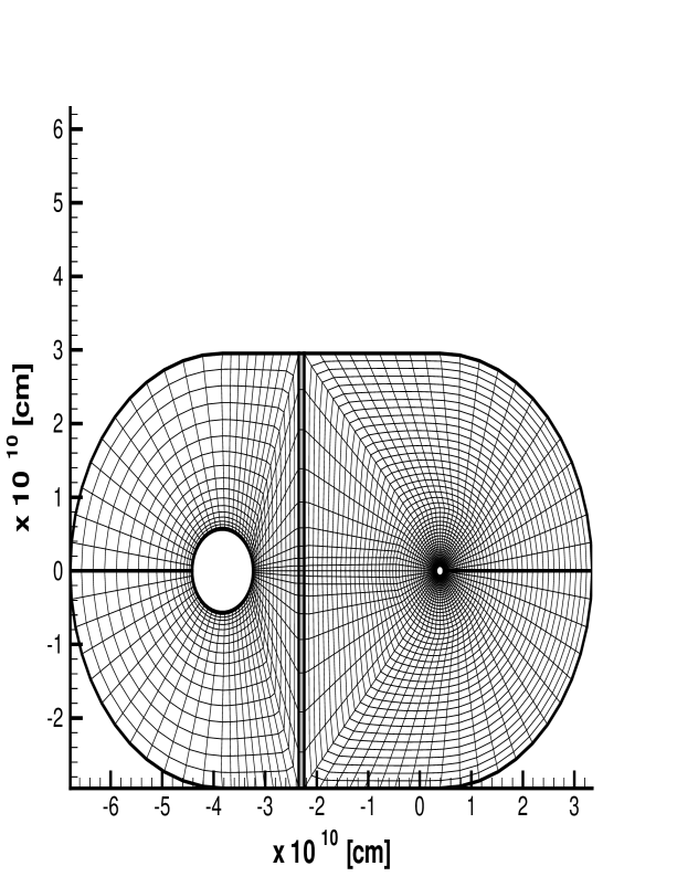
Figure 1: The generalized curvilinear coordinate used here. The mesh size is $20\times 61$ in the mass losing star region, $3\times 19$ in the connecting region and $44\times 61$ in the mass accreting star region.

A finite volume approach is used to discretize the governing equations. The AUSM-DV scheme is used to obtain the numerical convective flux (Wada & Liou, 1994). In the time integration, a matrix free LU-SGS method is employed (Nakahashi et al., 1999). Inner iterations are made to assure the second order temporal accuracy in the implicit integration (Yamamoto & Kano, 1996). A CFL number of $1000$ is assumed in the calculations.

The parameters that characterize the gas ejected from the mass losing component are the sound velocity, which is chosen to be $c_{0}=73[\mbox{km s}^{-1}]$, and the velocity of the gas inside of the star, which is $u_{0}=0$. Although we assume a stationary gas, the higher pressure inside of the mass losing star drives the gas flown into the computational domain. Note that if we employ $A\Omega$ as a typical velocity scale as was in the previous works, where $A$ is the separation of the two stars and $\Omega$ is the angular velocity of the system, the dimensionless sound velocity of the ejected gas becomes $0.15$. As a boundary condition at the surface of the mass accreting star as well as at the outer boundary of the computational domain, we assume a vacuum condition in which any gas reaching there is simply absorbed in. As an initial condition, we assume a gas with very low density, $0.5\times 10^{-14}[\mbox{g cm}^{-3}]$, and high temperature, $3.22\times 10^{6}/\gamma[\mbox{K}]$, that fills up the entire computational domain.

In order to avoid the numerical instability at the initial stage, we first calculate the flow of the gas with $\gamma=5/3$ without radiative cooling up to $10^{5}$ time steps using first-order-accurate scheme. After that we switch to second-order-accurate scheme. At the same time, the $\gamma$ value is changed for relevant cases. The radiative cooling effect is also included for non-adiabatic cases.

Our computational domain includes both the mass losing star and the mass accreting star on the equatorial plane (Fig. 1). The computational domain that contains the mass losing star has $20\times 61$ grid points, while that contains the mass accreting star has $44\times 61$ grid points. These two domains are connected by a narrow strip that has $3\times 19$ grid points.

2.2 NUMERICAL TREATMENT OF RADIATIVE TRANSFER

It is assumed that energy discharge due to radiative cooling occurs in the vertical directions from the top and bottom surfaces of the disc. Because the present flowfield is confined in a two-dimensional equatorial plan, it is necessary to assume the distribution of physical quantities in the vertical direction in the disc for calculation of radiation. We assume a hydrostatic balance in the vertical direction to determine the thickness of the disc, and that the physical quantities in the vertical direction are constant with the local values in the equatorial plan. The thickness of the disc $H$ is given by

$$H=\frac{c_{s}}{\Omega_{\mbox{K}}}=c_{s}\sqrt{\frac{r_{1}^{3}}{GM_{1}}},$$ (22)

where $c_{s}$, $\Omega_{\mbox{K}}$, $r_{1}$ and $G$ are the sound speed of the gas on the disc, the Keplerian frequency, the radial distance from the mass accreting star and the gravitational constant, respectively.

The coupling of the flowfield and the radiation field is occurred through the term of $\partial F_{z}/\partial z$ that appears in the energy equation. $\partial F_{z}/\partial z$ is obtained by solving the following equation for radiation energy

$$\frac{\partial F_{z}}{\partial z}=4\pi\chi B-c\chi E,$$ (23)

where $B$, $E$, $c$ and $\chi$ are the Planck function, the radiation energy density per unit volume, the speed of light and opacity, respectively. Because the speed of light is far larger than the sound velocity, and we only seek for a steady state solution, we ignore the time differential term that appears in the radiative transfer equation.

In the present work we employ the Kramer’s opacity which has no dependence on frequency. This Kramer’s opacity is suitable for the calculation of pure hydrogen gas above $10^{4}[\mbox{K}]$, and is written in the following form (Cannizzo, Shafter & Wheeler, 1988; Stehle, 1999)

$$\chi=2.8\times 10^{24}\rho^{2}T^{-3.5}[\mbox{cm}^{-1}],$$ (24)

where $T$ is the temperature of the gas.

As mentioned earlier, we consider the radiative transfer only in the vertical direction of the disc, i.e. the $z$ direction perpendicular to the $x\mbox{-}y$ plane. The radiative transfer within the disc is ignored. Moreover, the radiative transfer is taken into account in the calculations only in the computational domain that contains the mass accreting star and hence the accretion disc.

The radiative heat flux in the accretion disc is calculated by the FLD approximation (Alme & Wilson, 1974; Levermore & Pomraning, 1981). We assume the gas is in local thermodynamic equilibrium at a temperature that needs not correspond to that of the radiation field. This is because we solve the radiation energy equation (23) to determine the radiation energy density $E$. With the FLD approximation, the radiative flux can be written in the form of Fick’s law of diffusion (Levermore & Pomraning, 1981) as

$$F_{z}=-D\frac{\partial E}{\partial z},$$ (25)

with a diffusion coefficient, $D$, given by

$$D=\frac{c\lambda}{\chi}.$$ (26)

The dimensionless function $\lambda=\lambda(E)$ is called as the flux limiter. We employ Minerbo’s model (Minerbo, 1978) as a choice of $\lambda$, i.e. a constraint on the anisotropy of the radiation field. Minerbo assumed a piecewise linear variation of the specific intensity with angle, and found the functional form of the flux limiter as

$$\lambda(R)=\left\{\begin{array}[]{ll}2/(3+\sqrt{9+12R^{2}})&\quad\mbox{if}\quad 0\leq R\leq 3/2,\\ (1+R+\sqrt{1+2R})^{-1}&\quad\mbox{if}\quad 3/2<R<\infty,\end{array}\right.$$ (27)

where $R$ is a dimensionless quantity $R=\left|\partial E/\partial z\right|/(\chi E)$. In the optically thin limit $R\rightarrow\infty$, the flux limiter gives

$$\lim_{R\to\infty}\lambda(R)=\frac{1}{R},$$ (28)

to the first order in $R^{-1}$. The magnitude of the flux therefore approaches $\left|F_{z}\right|=c\left|\partial E/\partial z\right|/(\chi R)=cE$, which obeys the causality constraint. In the optically thick or diffusion limit $R\rightarrow 0$, the flux limiter gives

$$\lim_{R\to 0}\lambda(R)=\frac{1}{3},$$ (29)

to the first order in $R$, so that the flux takes the value given by equation (25).

The method of the solving the radiation energy equation (23) is described in Appendix A.

3 RESULTS

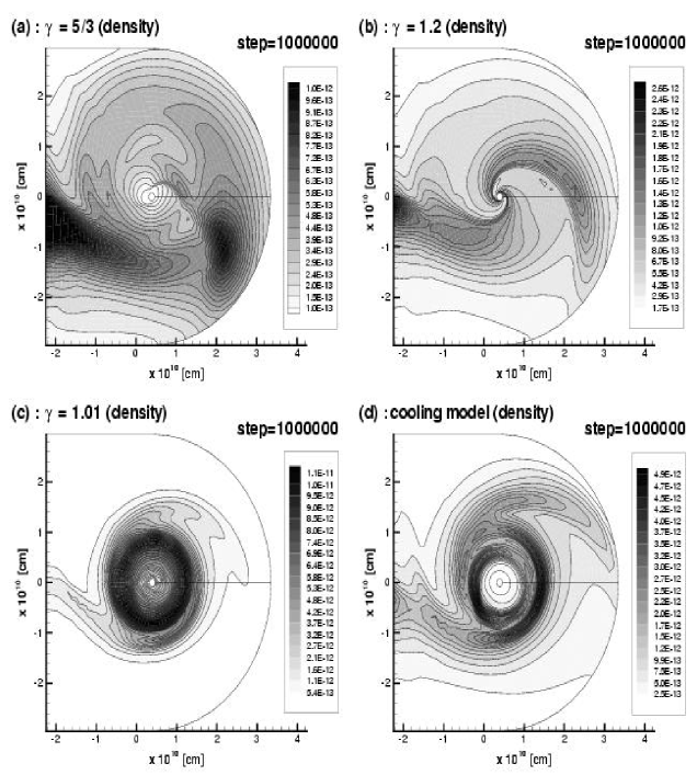
Figure 2: Density contours for each case. (a), (b) and (c) show the density contours for the cases of $\gamma=5/3$, $1.2$ and $1.01$ not accounting for the radiative cooling, respectively. (d) shows the density contours for the case of $\gamma=5/3$ accounting for the radiative cooling. The density range in (a), (b), (c) and (d) is from $1.0\times 10^{-13}$ to $1.0\times 10^{-12}$, from $1.7\times 10^{-13}$ to $2.6\times 10^{-12}$, from $5.4\times 10^{-13}$ to $1.1\times 10^{-11}$ and from $2.5\times 10^{-13}$ to $4.9\times 10^{-12}[\mbox{g cm}^{-3}]$, respectively. Each density range is divided by $20$ lines with an equal increment. The system rotates counterclockwise.

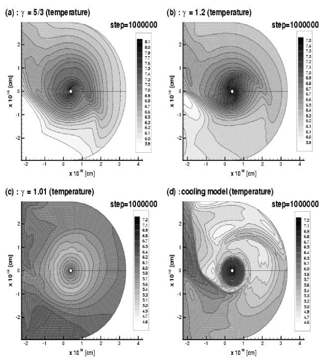
Figure 3: Temperature contours with logarithmic scale for each case. (a), (b) and (c) show the temperature contours for the cases of $\gamma=5/3$, $1.2$ and $1.01$ not accounting for the radiative cooling, respectively. (d) shows the temperature contours for the case of $\gamma=5/3$ accounting for the radiative cooling. The temperature range in (a), (b), (c) and (d) is from $\log_{10}T[\mbox{K}]=5.9$ to $8.1$, from $5.9$ to $7.5$, from $4.6$ to $7.2$ and from $4.6$ to $7.2$, respectively. The temperature range is divided by $20$ lines with an equal increment.

Figs. 2 (a), (b) and (c) show the density distribution in a (quasi) steady state (at $10^{6}$ step) for the cases of adiabatic gas with $\gamma=5/3$, $1.2$ and $1.01$, respectively. In these calculations radiative cooling effect is not included. It is shown that the disc structure is formed and the spiral shocks are appeared in each case. For the case of $\gamma=5/3$, the spiral arms are less clear as shown in Fig. 2 (a). This is because the contour lines are plotted at equal interval while the density in the disc for this case is relatively lower than that in the L1 stream.

It should be noted that the steady state is not steady in a strict sense, but slightly oscillates. Especially, for the case of $\gamma=5/3$, the density pattern and the shock position periodically change with time, although the general pattern in the inner and outer region remains unchanged. The temporal fluctuation of the disc structure, however, is not significant and the density distribution shown in Fig. 2 (a) gives a typical one for the case of $\gamma=5/3$. This is suggested by the fact that the present density distribution virtually coincides with that of the ensemble average taken from $2.0\times 10^{5}$ to $1.0\times 10^{6}$ time steps.

The pitch angle of spiral arms has a clear correlation with $\gamma$. The lower $\gamma$ thus leads to a tightly wound spiral shocks. These results are consistent with the previous works (Sawada, Matsuda & Hachisu, 1986a; Makita, Miyawaki & Matsuda, 1987).

The maximum Mach number in the disc is about $4$, $5$ and $23$ for the cases of $\gamma=5/3,1.2$ and $1.01$, respectively.

Fig. 2 (d) shows the density distribution for the case in which the specific heat ratio is fixed as $5/3$ and the effect of radiative cooing is accounted for. Obviously, one can see that the disc structure is formed and spiral shocks are appeared.

Spiral shocks disappear near the mass accreting star and nearly axisymmetric disc structure is formed. Those flow patterns are quite similar to that obtained in the calculation of adiabatic case with $\gamma=1.01$, although the absolute value of density in the disc becomes smaller.

The maximum Mach number in the disc is found to be $23$ for this case which is the same as that for the case of $\gamma=1.01$.

Figs. 3 (a), (b) and (c) show the temperature distribution in a (quasi) steady state with logarithmic scale for the cases of adiabatic gas with $\gamma=5/3$, $1.2$ and $1.01$, respectively. As can be seen in Fig. 3 (a) and (b), the temperature of the gas in the disc is very high and becomes above $10^{7}[\mbox{K}]$ near the mass accreting star. The smaller $\gamma$ value for this case results in nearly isothermal distribution in the disc that gives substantially lower temperature near the mass accreting star. As shown in Fig. 3 (c), compared with the other adiabatic cases, the temperature distribution for the case of $\gamma=1.01$ is found to be close to flat.

Fig. 3 (d) shows the temperature distribution with logarithmic scale in a (quasi) steady state for the case of $\gamma=5/3$ with radiative cooling. Compared with the other adiabatic cases without radiative cooling, the temperature in the accretion disc is significantly lowered to less than $10^{5}[\mbox{K}]$, except for the small disc region near the mass accreting star where the temperature exceeds $10^{7}[\mbox{K}]$. In other words, the accretion disc exhibits a dual structure, i.e. the significantly cooled outer region and the inner core region where temperature is very high. The precise structure in the inner core region, however, is difficult to resolve with the present mesh system, because the pitch angle of the spiral shocks becomes smaller as approaches to the inner region.

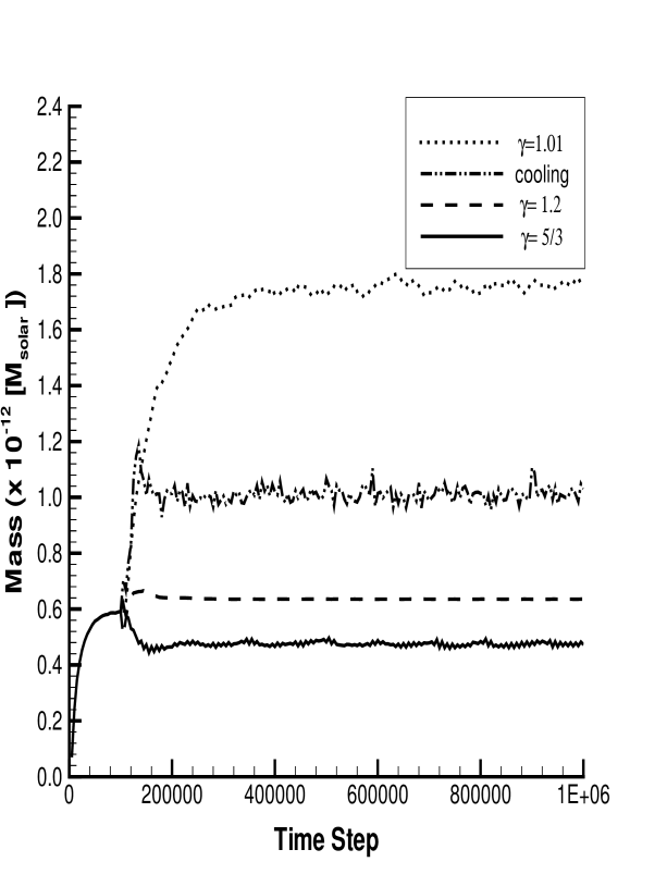
Figure 4: The evolution of the total mass in the mass accreting region denoted by solar mass unit. The total mass is defined as a sum of all the masses in the mass accreting region.

The evolution of the total mass in the mass accreting region is shown for each case in Fig. 4. The total mass is defined as a sum of all the masses in the mass accreting region. The horizontal axis denotes the time step. $1.0\times 10^{6}$ time steps correspond to more than $700$ orbital periods. In all the cases, the total mass in the mass accreting region becomes almost constant after $3.0\times 10^{5}$ time steps but begin to oscillate slightly around each mean value. Therefore, we can say that each flowfield in the accretion disc reaches a (quasi) steady state. The total mass for the case accounting for radiative cooling is found to be larger than that for the case of $\gamma=1.2$, and smaller than that for the case of $\gamma=1.01$. From the results, we can say that the overall behavior of the flowfield as well as the evolution of the total mass of the adiabatic case with a smaller $\gamma$ value is quite similar to the one with radiative cooling shown in the present study. Although the precise $\gamma$ value can change for case-to-case, one can conclude that the use of a lower $\gamma$ value for simulating radiative cooling effect is almost a valid assumption.

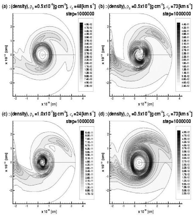
Figure 5: Density contours for the case of $\gamma=5/3$ accounting for the radiative cooling for the different parameters of $\rho_{0}$ and $c_{0}$. (a), (b), (c) and (d) show the density contour for the cases of $(\rho_{0},c_{0})=(0.5\times 10^{-9},48),(0.5\times 10^{-8},73),(1.0\times 10^{-7},24)$ and $(0.5\times 10^{-9}[\mbox{g cm}^{-3}],73[\mbox{km s}^{-1}])$, respectively. The figure of (d) is same as that of Fig. 2 (d), which is the standard case. The density range in (a), (b) and (c) is from $2.5\times 10^{-13}$ to $4.9\times 10^{-12}$, from $2.4\times 10^{-12}$ to $4.4\times 10^{-11}$ and from $4.7\times 10^{-12}$ to $8.4\times 10^{-11}[\mbox{g cm}^{-3}]$, respectively. The density range in (d) is same as it of (b). Each density range is divided by $20$ lines with an equal increment.

Finally, let us examine the influence of gas properties from the mass losing star. Because the process of discharge and absorption of radiation depends on density and temperature of the gas in the accretion disc that is influenced primarily by the gas from the mass losing star, we need to know what are the consequences of changing properties of the gas. Fig. 5 (a) shows the density contours in the accretion disc for the lower temperature case in which $\rho_{0}=0.5\times 10^{-9}[\mbox{g cm}^{-3}]$ and $c_{0}=48[\mbox{km s}^{-1}]$. In the calculation, the radiative cooling effect is considered. In this case, the accretion disc slightly shrinks, but the overall feature is unchanged if compared with the standard case shown in Fig. 5 (d). On the other hand, if we increase the surface density of the mass losing star, some changes are seen in the results. Fig. 5 (b) shows the density contours for the case with $\rho_{0}=0.5\times 10^{-8}[\mbox{g cm}^{-3}]$ and $c_{0}=73[\mbox{km s}^{-1}]$. Note that the density scale is changed to show the overall distribution. In this case, the inner disc region again appears where density becomes very low, but its radius becomes smaller. Surrounding this inner region, there appear several spiral arms in the intermediate region. This intermediate region has a ring like structure, which is connected to an outer spiral arm and also to the incoming flow from the L1point. In Fig. 5 (c), the density contours for the limiting case of $\rho_{0}=1.0\times 10^{-7}[\mbox{g cm}^{-3}]$ and $c_{0}=24[\mbox{km s}^{-1}]$ are shown. One can see that the overall feature is quite similar to that shown in Fig. 5 (b), though the inner disc region further shrinks.

4 CONCLUDING REMARKS

Two-dimensional hydrodynamic calculations of an invisicid flowfield in a close binary system are carried out by solving the Euler equations with radiative transfer. In the present study, the specific heat ratio is assumed to be constant while radiative cooling effect is included as a non-adiabatic process. The cooling effect of the disc is considered by discharging energy in the vertical directions from the top and bottom surfaces of the disc. We use the flux-limited diffusion approximation to calculate the radiative heat flux values. The obtained results are summarized as follows:

(i)

Around the mass accreting star, there appears an accretion disc and spiral shocks are formed in the disc, even for the case with radiative cooling.

(ii)

The total mass of the disc reaches a (quasi) steady value. It becomes larger when radiative cooling effect is accounted for than that assuming $\gamma=5/3$, and is close to the value for the case of lower $\gamma$.

(iii)

The lower $\gamma$ value for an adiabatic gas which has been employed in the simulation of accretion discs in order to account for radiative cooling effect is found to be almost a valid assumption in terms of the overall flow features and also the amount of the total mass.

What are shown in this work are the results of two-dimensional hydrodynamic calculation of inviscid flowfield accounting for radiative cooling effect. In order to obtain more rigorous results for the accreting flowfield, we need to explore three-dimensional flowfield that is coupled with radiative transfer. In such case, one needs to account for radiative transfer that is parallel to equatorial plane. This is because the accretion disc is not necessarily a flat thin disc. It is also needed to employ a more detailed radiation model that can consider spectral dependence of opacity. For such calculation, a flux-limited diffusion model is no more applicable and we need further to employ a detailed simulation method such as to use ray-tracing technique to solve radiative transfer equations. Our future studies will focus on these aspects.

Appendix A Discretizing of Radiation Energy Equation

Let us consider the method of solving the radiation energy equation (23). Using the flux-limited diffusion approximation (25), equation (23) can be rewritten in the following form for radiation energy density $E$ as

$$-\frac{\partial}{\partial z}\left(D\frac{\partial E}{\partial z}\right)=4\pi\chi B-c\chi E.$$ (30)

Because the distribution of physical quantities in the vertical direction is assumed to be constant, the diffusion coefficient $D$ is independent of the height $z$. Therefore, we replace the partial differential in $z$ by multiplying $1/H$. As a result, equation (30) is discretized as

$$2D^{n}\frac{E^{n+1}}{(H^{n})^{2}}=4\pi\chi^{n}B^{n}-c\chi^{n}E^{n+1},$$ (31)

where the superscript $n$ denotes the time step. The factor $2$ in the left hand side of the equation (31) appears because discharging energy by radiation occurs from the top and bottom surfaces of the disc. Except for the radiation energy density $E$, the dependent variables are evaluated at time step $n$. Equation (31) is solved for $E^{n+1}$. This $E^{n+1}$ is substituted into the discrete form of $\partial F_{z}/\partial z$, i.e. $2D^{n}E^{n+1}/(H^{n})^{2}$ which is further substituted into the energy equation of the Euler equations. This completes the coupling procedure of the flowfield with radiation.

References

- Alme & Wilson (1974) Alme M. L., Wilson J. R., 1974, ApJ, 194, 147