Measurements of Proton, Helium and Muon Spectra at Small Atmospheric Depths with the BESS Spectrometer

Abstract

The cosmic-ray proton, helium, and muon spectra at small atmospheric depths of 4.5 – 28 g/cm² were precisely measured during the slow descending period of the BESS-2001 balloon flight. The variation of atmospheric secondary particle fluxes as a function of atmospheric depth provides fundamental information to study hadronic interactions of the primary cosmic rays with the atmosphere.

, , , , , , , , , , , , , , , , , , , , , , , , , , , , , , , , , ,

1 Introduction

Primary cosmic rays interact with nuclei in the atmosphere, and produce atmospheric secondary particles, such as muons, gamma rays and neutrinos. It is important to understand these interactions to investigate cosmic-ray phenomena inside the atmosphere. For precise study of the atmospheric neutrino oscillation [1], it is crucial to reduce uncertainties in hadronic interactions, which are main sources of systematic errors in the prediction of the energy spectra of atmospheric neutrinos. At small atmospheric depths below a few ten g/cm², production process of muons is predominant over decay process, thus we can clearly observe a feature of the hadronic interactions. In spite of their importance, only a few measurements have been performed with modest statistics because of strong constraints of short observation time of a few hours during balloon ascending periods from the ground to the balloon floating altitude.

In 2001, using the BESS spectrometer, precise measurements of the cosmic-ray fluxes and their dependence on atmospheric depth were carried out during slow descending from 4.5 g/cm² to 28 g/cm² for 12.4 hours. The growth curves of the cosmic-ray fluxes were precisely measured. The results were compared with the predictions based on the hadronic interaction models currently used in the atmospheric neutrino flux calculations.

2 BESS spectrometer

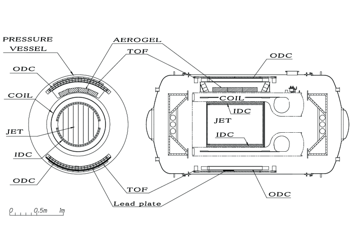
Figure 1: Cross sectional view of the BESS detector.

The BESS ($\underline{\rm B}$alloon-borne $\underline{\rm E}$xperiment with a $\underline{\rm S}$uperconducting $\underline{\rm S}$pectrometer) detector [2, 3, 4, 5, 6] is a high-resolution spectrometer with a large acceptance to perform precise measurement of absolute fluxes of various cosmic rays [7, 8, 9], as well as highly sensitive searches for rare cosmic-ray components. Fig. 1 shows a schematic cross-sectional view of the BESS instrument. In the central region, a uniform magnetic field of 1 Tesla is provided by a thin superconducting solenoidal coil. The magnetic-rigidity ($R\equiv Pc/Ze$) of an incoming charged particle is measured by a tracking system, which consists of a jet-type drift chamber (JET) and two inner-drift-chambers (IDC’s) inside the magnetic field. The deflection ($R^{-1}$) is calculated for each event by applying a circular fitting using up-to 28 hit-points, each with a spatial resolution of 200 $\mu$m. The maximum detectable rigidity (MDR) was estimated to be 200 GV. Time-of-flight (TOF) hodoscopes provide the velocity ($\beta$) and energy loss ($\d E/\d x$) measurements. A 1/$\beta$ resolution of 1.4 % was achieved in this experiment. For particle identification, the BESS spectrometer was equipped with a threshold-type aerogel Cherenkov counter and an electromagnetic shower counter. The refractive index of silica aerogel radiator was 1.022, and the threshold kinetic energy for proton was 3.6 GeV. The shower counter consists of a plate of lead with two radiation lengths covering a quarter area of the lower TOF counters, whose output signal was utilized for $e$/$\mu$ identification.

The data acquisition sequence is initiated by a first-level TOF trigger, which is a simple coincidence of signals in the upper and lower TOF counter. In order to build a sample of unbiased triggers, one of every four events were recorded. The TOF trigger efficiency was evaluated to be 99.4 % $\pm$ 0.2 % by using secondary proton beam at the KEK 12 GeV proton synchrotron. In addition to the TOF trigger, an auxiliary trigger is generated by a signal from the Cherenkov counter to record particles above threshold energy without bias or sampling. An efficiency of Cherenkov trigger were evaluated as a ratio of the Cherenkov-triggered events among the unbiased trigger sample. It was 95.1 % for relativistic particles ($\beta\rightarrow 1$). For flux determinations, the Cherenkov-triggered events were used only above 9.5 GV for protons, 11.1 GV for helium nuclei, and 0.90 GV for muons. Below these rigidities, the TOF-triggered events were used.

3 Balloon flight

The BESS-2001 balloon flight was carried out at Ft. Sumner, New Mexico, USA (34^∘49^′N, 104^∘22^′W) on 24th September 2001. Throughout the flight, the vertical geomagnetic cut-off rigidity was about 4.2 GV. The balloon reached at a normal floating altitude of 36 km at an atmospheric depth of 4.5 g/cm². After a few hours, the balloon started to lose the floating altitude and continued descending for more than 13 hours until termination of the flight. During the descending period, data were collected at atmospheric depths between 4.5 g/cm² and 28 g/cm². The atmospheric depth was measured with accuracy of $\pm$ 1 g/cm², which comes mainly from an error in absolute calibration of an environmental monitor system. Fig. 2 shows a balloon flight profile during the experiment.

4 Data analysis

4.1 Data reduction

We selected “non-interacted” events passing through the detector without any interactions. The non-interacted event was defined as an event, which has only one isolated track, one or two hit-counters in each layer of the TOF hodoscopes, and proper d$E$/d$x$ inside the upper TOF counters. There is a slight probability that particles interact with nuclei in the detector material and only one secondary particle goes into the tracking volume to be identified as a non-interacted event. These events were rejected by requiring proper d$E$/d$x$ inside the upper TOF counters, because the interaction in the detector is expected to give a large energy deposit in the TOF counter. According to the Monte Carlo simulation with GEANT [10], these events are to be considered only below a few GeV. In order to estimate an efficiency of the non-interacted event selection, Monte Carlo simulations were performed. The probability that each particle can be identified as a non-interacted event was evaluated by applying the same selection criterion to the Monte Carlo events as was applied to the observed data. The systematic error was estimated by comparing the hit number distribution of the TOF counters. For muons, the simulated data were compared with muon data sample measured on the ground. The systematic error for protons below 1 GeV was directly determined by the detector beam test using accelerator proton beam [11]. The resultant efficiency and its error of non-interacted event selection for protons was 83.3 $\pm$ 2.0 % at 1.0 GeV and 77.4 $\pm$ 2.5 % at 10 GeV, and that for helium nuclei was 71.6 $\pm$ 2.6 % at 1.0 GeV/n and 66.0 $\pm$ 2.9 % at 10 GeV/n. The efficiency for muons was 94.0 $\pm$ 0.9 % and 92.8 $\pm$ 0.8 % at 0.5 GeV and 10 GeV, respectively.

The selected non-interacted events were required to pass through the fiducial volume defined in this analysis. The fiducial volume of the detector was limited to the central region of the JET chamber for a better rigidity measurement. The zenith angle ($\theta_{z}$) was limited within $\cos\theta_{z}\geq 0.90$ to obtain nearly vertical fluxes. For the muon analysis, we used only the particles which passed through the lead plate to estimate electron contaminations. For the proton and helium analysis, particles were required not to pass through the lead plate so as to keep the interaction probability inside the detector as low as possible.

In order to check the track reconstruction efficiency inside the tracking system, the recorded events were scanned randomly. It was confirmed that 996 out of 1,000 visually identified tracks which passed through the fiducial volume were successfully reconstructed, thus the track reconstruction efficiency was evaluated to be 99.6 $\pm$ 0.2 %. It was also confirmed that rare interacted events are fully eliminated by the non-interacted event selection.

4.2 Particle identification

In order to select singly and doubly charged particles, particles were required to have proper d$E$/d$x$ as a function of rigidity inside both the upper and lower TOF hodoscopes. The upper TOF d$E$/d$x$ was already examined in the non-interacted event selection. The distribution of d$E$/d$x$ inside the lower TOF counter and the selection boundaries are shown in Fig. 3.

In order to estimate efficiencies of the d$E$/d$x$ selections for protons and helium nuclei, we used another data sample selected by independent information of energy loss inside the JET chamber. The estimated efficiency in the d$E$/d$x$ selection at 1 GeV was 98.3 $\pm$ 0.4 % and 97.2 $\pm$ 0.5 % for protons and helium nuclei, respectively. The accuracy of the efficiency for protons and helium nuclei was limited by statistics of the sample events. Since muons could not be distinguished from electrons by the JET chamber, the d$E$/d$x$ selection efficiency for muons was estimated by the Monte Carlo simulation to be 99.3 $\pm$ 1.0 %. The error for muons comes from the discrepancy between the observed and simulated d$E$/d$x$ distribution inside the TOF counters. The d$E$/d$x$ selection efficiencies were almost constant in the whole energy region discussed here.

Particle mass was reconstructed by using the relation of 1/$\beta$, rigidity and charge, and was required to be consistent with protons, helium nuclei or muons. An appropriate relation between 1/$\beta$ and rigidity for each particle was required as shown in Fig. 4. Since the 1/$\beta$ distribution is well described by Gaussian and a half-width of the 1/$\beta$ selection band was set at 3.89 $\sigma$, the efficiency is very close to unity (99.99 % for pure Gaussian).

4.3 Contamination estimation

4.3.1 Protons

Protons were clearly identified without any contamination below 1.7 GV by the mass selection, as shown in Fig. 4. Above 1.7 GV, however, light particles such as positrons and muons contaminate proton’s $1/\beta$-band, and above 4 GV deuterons ($D$’s) start to contaminate it.

To distinguish protons from muons and positrons above 1.7 GV, we required that light output of the aerogel Cherenkov counter should be smaller than the threshold. This requirement rejected 96.5 % of muons and positrons while keeping the efficiency for protons as high as 99.5 %. The aerogel Cherenkov cut was applied below 3.7 GV, above which Cherenkov output for protons begins to increase rapidly.

Contamination of muons in proton candidates after the aerogel Cherenkov cut was estimated and subtracted by using calculated muon fluxes [20], which was normalized to the observed fluxes below 1.0 GeV where positive muons were clearly separated from protons. The positron contamination was calculated from the normalized positive muon fluxes and observed $e$/$\mu$ ratios. The resultant positive muon and positron contamination in the proton candidates was less than 0.8 % and 4.1 % below and above 3.7 GV, respectively, at 26.4 g/cm² where observed $(\mu$+$e)$/$p$ ratio is largest during the experiment. The error in this subtraction was estimated from the ambiguity in the normalization of the muon spectra to be less than 0.2 % and 0.8 % below and above 3.7 GV, respectively.

Since the geomagnetic cut-off rigidity is 4.2 GV, most of deuterons contaminating proton candidates above 4 GV are considered to be primary cosmic-ray particles. The primary $D$/$p$ ratio was estimated by our previous measurement carried out in 1998 – 2000 at Lynn Lake, Manitoba, Canada, where the cut-off rigidity is as low as 0.5 GV. The $D$/$p$ ratio was found to be 2 % at 3 GV. No subtraction was made for deuteron contamination because there is no reliable measurement of the deuteron flux above 4 GV. Therefore, above 4 GV hydrogen nuclei selected which included a small amount of deuterons. The $D$/$p$ ratio at higher energy is expected to decrease [12] due to the decrease in escape path lengths of primary cosmic-ray nuclei [13] and the deuteron component is as small as the statistical error of the proton flux.

4.3.2 Helium nuclei

Helium nuclei were clearly identified by using both upper and lower TOF d$E$/d$x$ as shown in Fig. 3. Landau tail in proton’s d$E$/d$x$ might contaminate the helium d$E$/d$x$ band, however this contamination from protons was as small as 3$\times$10^-4. It was estimated by using another sample of proton data selected by d$E$/d$x$ in the JET chamber. No background subtraction was made for helium. Obtained helium fluxes include both ³He and ⁴He.

4.3.3 Muons

Electrons and pions could contaminate muon candidates. To estimate electron contamination, we used the d$E$/d$x$ information inside the lower TOF counters covered with the lead plate. We calculated lower TOF d$E$/d$x$ distribution for muons and electrons using the Monte Carlo simulation. The most adequate e/$\mu$ ratio was estimated by changing weights both for muons and electrons so as to reproduce the observed d$E$/d$x$ distribution. The simulated distributions well-agreed with the observed data as shown in Fig. 5. The electron contamination was about 10 % of muon candidates at 0.5 GV, and less than 1% above 1 GV. Since in the lower energy region, the difference between the d$E$/d$x$ distributions for electrons and muons are small, rejection power of d$E$/d$x$ selection are lower. The error was estimated during the fitting procedure to be about 5 % at 0.5 GV and 0.1 % at 8.0 GV. Accuracy of the electron subtraction was limited by poor statistics of electron events. For the pion contamination we made no subtraction, thus the observed muon fluxes include pions. According to a theoretical calculation [14], the $\pi$/$\mu$ ratio at a residual atmosphere of 3 g/cm² through 10 g/cm² was less than 3 % at 1 GV and less than 10 % at 10 GV.

Between 1.6 and 2.6 GV, protons contamination in the positive muon candidates and its error were estimated by fitting the 1/$\beta$ distribution with a double-Gaussian function as shown in Fig 6. The estimated ratio of proton contamination in muon candidates was less than 3.3 $\pm$ 1.3 %.

4.4 Corrections

In order to determine the proton, helium and muon spectra, ionization energy loss inside the detector material, live-time and geometrical acceptance need to be estimated.

The energy of each particle at the top of the instrument was calculated by summing up the ionization energy losses inside the instrument with tracing back the event trajectory. The total live data-taking time was measured exactly to be 40,601 seconds by counting 1 MHz clock pulses with a scaler system gated by a “ready” status that control the first level trigger. The geometrical acceptance defined for this analysis was calculated as a function of rigidity by using simulation technique [15]. In the high rigidity region where a track of the particle is nearly straight, the geometrical acceptance is 0.097 ${\mathrm{m^{2}sr}}$ for protons and helium nuclei, and 0.030 ${\mathrm{m^{2}sr}}$ for muons. The acceptance for muons is about 1/3 of that for protons and helium nuclei, because we required muons to pass through the lead plate while protons and helium nuclei were required not to pass through the lead plate. The simple cylindrical shape and the uniform magnetic field make it simple and reliable to determine the precise geometrical acceptance. The error which arose from uncertainty of the detector alignment was estimated to be 1 %.

5 Results and discussions

The proton and helium fluxes in energy ranges of 0.5–10 GeV/n and muon flux in 0.5 GeV/$c$–10 GeV/$c$, at small atmospheric depths of 4.5 g/cm² through 28 g/cm², have been obtained from the BESS-2001 balloon flight. The results are summarized in Table 1. The statistical errors were calculated as 68.7 % confidence interval based on Feldman and Cousins’s “unified approach” [16]. The overall errors including both statistic and systematic errors are less than 8 %, 10% and 20 % for protons, helium nuclei and muons, respectively. The obtained proton and helium spectra are shown in Fig. 7. Around at 3.4 GeV for protons and 1.4 GeV/n for helium nuclei, a geomagnetic cut-off effect is clearly observed in their spectra. The proton spectrum measured by the AMS experiment in 1998 [17] at the similar geomagnetic latitude ($0.7<\Theta_{M}<0.8$, where $\Theta_{M}$ is the corrected geomagnetic latitude [18]) is also shown in Fig. 7. The AMS measured proton spectra in space (at an altitude of 380 km), which are free from atmospheric secondary particles. In the BESS results the atmospheric secondary spectra for protons below 2.5 GeV are observed. Fig. 8 shows the observed proton and helium fluxes as a function of the atmospheric depth. Below 2.5 GeV the proton fluxes clearly increase as the atmospheric depth increases. It is because the secondary protons are produced in the atmosphere. In the primary fluxes above the geomagnetic cut-off, the fluxes attenuate as the atmospheric depth increases. In this energy region, the production of the secondary protons is much smaller than interaction loss of the primary protons. This is because the flux of parent particles of secondary protons is much smaller due to the steep spectrum of primary cosmic rays.

Figs. 10 and 10 show the observed muon spectra together with theoretical predictions. The predictions were made with the hadronic interaction model, DPMJET-III [19], which was used for the evaluation of atmospheric neutrino fluxes [20]. The obtained proton fluxes were used to reproduce the primary cosmic-ray fluxes in the calculation. Fig. 11 shows the observed muon fluxes as a function of atmospheric depth together with the calculated fluxes. The calculated fluxes show good agreement with the observed data. Further detailed study of the hadronic interaction models will be discussed elsewhere.

6 Conclusion

We made precise measurements of cosmic-ray spectra of protons, helium nuclei and muons at small atmospheric depths of 4.5 through 28 g/cm², during a slow descending period of 12.4 hours, in the BESS-2001 balloon flight at Ft. Sumner, New Mexico, USA. We obtained the proton and helium fluxes with overall errors of 8 % and 10 %, respectively, in an energy region of 0.5 – 10 GeV/n. The muon fluxes were obtained with an overall error of 20 % in a momentum region of 0.5 – 10 GeV/$c$. The results provide fundamental information to investigate hadronic interactions of cosmic rays with atmospheric nuclei. The measured muon spectra showed good agreement with the calculations by using the DPMJET-III hadronic interaction model. The understanding of the interactions will improve the accuracy of calculation of atmospheric neutrino fluxes.

Figure 2: Altitude during the BESS-2001 balloon flight experiment(top). Temperature and residual atmosphere as a function of altitude(bottom).

Figure 3: Distribution of d$E$/d$x$ inside the lower TOF counters. Solid lines show selection boundaries for protons and helium nuclei. Dashed lines show those for muons.

Figure 4: Distribution of 1/$\beta$ for $Z$=1 particles. Solid lines show the selection boundaries for protons. Dashed lines show those for muons.

Figure 5: Observed and simulated distribution of d$E$/d$x$ inside the lower TOF counters for the events in which track passed through the lead plate. Dashed line shows the selection boundary for muon. The observed data were summed up irrespective of the residual atmosphere.

Figure 6: An estimation of proton contamination by the TOF information. Hatched area shows an estimated proton contamination.

Figure 7: The observed proton and helium spectra. The error bars include statistical error only. In the proton spectra, atmospheric secondary components are clearly observed below 2.5 GeV in the BESS results.

Figure 8: The observed proton and helium fluxes as a function of atmospheric depth.

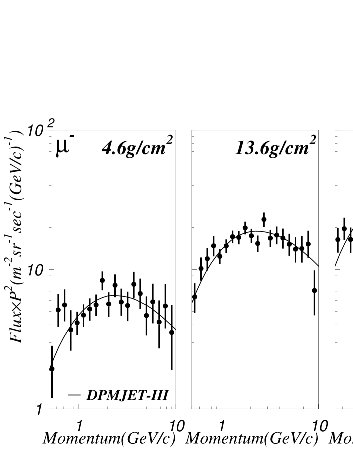
Figure 9: The observed negative muon spectra. The solid lines show theoretical predictions calculated by using DPMJET-III.

Figure 10: The observed positive muon spectra. The error bars include statistical error only. The solid lines show theoretical predictions calculated by using DPMJET-III.

Figure 11: The observed negative and positive muon fluxes. The solid lines show theoretical predictions calculated by using DPMJET-III.

Table 1: Observed proton fluxes

Energy range (GeV)	Flux$\pm~{}\Delta$Flux${}_{\rm sta}\pm~{}\Delta$Fluxsys (m-2sr-1s-1GeV-1)
	atmospheric depth range [mean] (g/cm2)
	4.46–4.80	4.86–7.21	7.04–8.23	8.24–9.08	9.06–9.54	9.60–11.4	11.4–12.5	12.7–14.6	14.7–16.4	16.5–19.8	21.2–25.0	25.0–28.2
	[4.58]	[5.82]	[7.81]	[8.70]	[9.33]	[10.4]	[11.9]	[13.6]	[15.6]	[17.6]	[23.4]	[26.4]
0.46– 0.54	40.8${}^{+3.3+0.9}_{-3.1-0.9}$	52.5${}^{+3.7+1.2}_{-3.5-1.2}$	63.0${}^{+3.8+1.4}_{-3.6-1.4}$	66.7${}^{+3.4+1.5}_{-3.2-1.5}$	68.3${}^{+4.3+1.6}_{-4.0-1.6}$	77.2${}^{+4.5+1.8}_{-4.2-1.8}$	96.7${}^{+4.9+2.2}_{-4.7-2.2}$	97.5${}^{+5.0+2.2}_{-4.8-2.2}$	114.${}^{+5.+3.}_{-5.-3.}$	125.${}^{+5.+3.}_{-5.-3.}$	141.${}^{+8.+3.}_{-8.-3.}$	178.${}^{+9.+4.}_{-9.-4.}$
0.54– 0.63	35.6${}^{+2.8+0.8}_{-2.6-0.8}$	41.0${}^{+3.0+0.9}_{-2.8-0.9}$	59.1${}^{+3.4+1.4}_{-3.2-1.4}$	57.1${}^{+2.9+1.3}_{-2.7-1.3}$	64.4${}^{+3.8+1.5}_{-3.6-1.5}$	69.7${}^{+3.9+1.6}_{-3.7-1.6}$	79.5${}^{+4.1+1.8}_{-3.9-1.8}$	79.9${}^{+4.1+1.8}_{-3.9-1.8}$	97.5${}^{+4.6+2.2}_{-4.4-2.2}$	101.${}^{+4.+2.}_{-4.-2.}$	134.${}^{+7.+3.}_{-7.-3.}$	141.${}^{+7.+3.}_{-7.-3.}$
0.63– 0.74	30.7${}^{+2.4+0.7}_{-2.2-0.7}$	34.0${}^{+2.5+0.8}_{-2.3-0.8}$	46.6${}^{+2.8+1.1}_{-2.6-1.1}$	50.7${}^{+2.5+1.2}_{-2.4-1.2}$	50.4${}^{+3.1+1.2}_{-2.9-1.2}$	58.9${}^{+3.3+1.3}_{-3.1-1.3}$	61.6${}^{+3.3+1.4}_{-3.2-1.4}$	68.2${}^{+3.5+1.6}_{-3.3-1.6}$	80.7${}^{+3.9+1.8}_{-3.7-1.8}$	91.2${}^{+3.7+2.1}_{-3.6-2.1}$	98.5${}^{+5.7+2.3}_{-5.4-2.3}$	124.${}^{+6.+3.}_{-6.-3.}$
0.74– 0.86	26.3${}^{+2.1+0.6}_{-1.9-0.6}$	31.9${}^{+2.2+0.7}_{-2.1-0.7}$	40.5${}^{+2.4+0.9}_{-2.2-0.9}$	44.1${}^{+2.1+1.0}_{-2.0-1.0}$	44.2${}^{+2.7+1.0}_{-2.5-1.0}$	52.9${}^{+2.8+1.2}_{-2.7-1.2}$	58.7${}^{+3.0+1.3}_{-2.8-1.3}$	61.6${}^{+3.1+1.4}_{-2.9-1.4}$	69.0${}^{+3.3+1.6}_{-3.1-1.6}$	74.3${}^{+3.1+1.7}_{-3.0-1.7}$	89.9${}^{+5.0+2.1}_{-4.7-2.1}$	103.${}^{+5.+2.}_{-5.-2.}$
0.86– 1.00	20.8${}^{+1.7+0.5}_{-1.6-0.5}$	25.8${}^{+1.9+0.6}_{-1.7-0.6}$	36.4${}^{+2.1+0.8}_{-2.0-0.8}$	38.9${}^{+1.8+0.9}_{-1.7-0.9}$	37.2${}^{+2.2+0.9}_{-2.1-0.9}$	46.7${}^{+2.5+1.1}_{-2.3-1.1}$	52.4${}^{+2.6+1.2}_{-2.5-1.2}$	52.8${}^{+2.6+1.2}_{-2.5-1.2}$	59.1${}^{+2.8+1.4}_{-2.7-1.4}$	63.4${}^{+2.6+1.5}_{-2.5-1.5}$	76.3${}^{+4.3+1.7}_{-4.0-1.7}$	83.0${}^{+4.5+1.9}_{-4.3-1.9}$
1.00– 1.17	21.7${}^{+1.6+0.4}_{-1.5-0.4}$	26.4${}^{+1.7+0.5}_{-1.6-0.5}$	30.2${}^{+1.7+0.5}_{-1.7-0.5}$	36.2${}^{+1.6+0.6}_{-1.6-0.6}$	37.5${}^{+2.1+0.7}_{-2.0-0.7}$	41.1${}^{+2.1+0.7}_{-2.0-0.7}$	45.7${}^{+2.2+0.8}_{-2.1-0.8}$	49.2${}^{+2.3+0.9}_{-2.2-0.9}$	48.6${}^{+2.4+0.8}_{-2.2-0.8}$	54.3${}^{+2.2+1.0}_{-2.2-1.0}$	70.3${}^{+3.7+1.2}_{-3.6-1.2}$	74.9${}^{+3.9+1.3}_{-3.7-1.3}$
1.17– 1.36	16.1${}^{+1.3+0.3}_{-1.2-0.3}$	20.8${}^{+1.4+0.4}_{-1.3-0.4}$	30.0${}^{+1.6+0.5}_{-1.5-0.5}$	30.5${}^{+1.4+0.5}_{-1.3-0.5}$	31.1${}^{+1.7+0.6}_{-1.7-0.6}$	35.6${}^{+1.8+0.6}_{-1.7-0.6}$	35.8${}^{+1.8+0.6}_{-1.7-0.6}$	43.0${}^{+2.0+0.8}_{-1.9-0.8}$	45.7${}^{+2.1+0.8}_{-2.0-0.8}$	48.8${}^{+2.0+0.9}_{-1.9-0.9}$	56.6${}^{+3.1+1.0}_{-3.0-1.0}$	71.7${}^{+3.5+1.3}_{-3.4-1.3}$
1.36– 1.58	14.8${}^{+1.1+0.3}_{-1.0-0.3}$	18.3${}^{+1.2+0.3}_{-1.2-0.3}$	22.8${}^{+1.3+0.4}_{-1.2-0.4}$	27.8${}^{+1.2+0.5}_{-1.2-0.5}$	24.9${}^{+1.4+0.4}_{-1.4-0.4}$	31.0${}^{+1.6+0.6}_{-1.5-0.6}$	35.2${}^{+1.7+0.6}_{-1.6-0.6}$	36.4${}^{+1.7+0.7}_{-1.6-0.7}$	43.1${}^{+1.9+0.8}_{-1.8-0.8}$	46.4${}^{+1.8+0.8}_{-1.7-0.8}$	56.2${}^{+2.9+1.0}_{-2.7-1.0}$	58.5${}^{+3.0+1.1}_{-2.8-1.1}$
1.58– 1.85	13.8${}^{+1.0+0.3}_{-0.9-0.3}$	15.3${}^{+1.0+0.3}_{-1.0-0.3}$	21.4${}^{+1.2+0.4}_{-1.1-0.4}$	21.8${}^{+1.0+0.4}_{-1.0-0.4}$	25.2${}^{+1.3+0.5}_{-1.3-0.5}$	26.4${}^{+1.4+0.5}_{-1.3-0.5}$	27.8${}^{+1.4+0.5}_{-1.3-0.5}$	33.3${}^{+1.5+0.6}_{-1.5-0.6}$	36.1${}^{+1.6+0.7}_{-1.5-0.7}$	39.8${}^{+1.5+0.7}_{-1.5-0.7}$	48.1${}^{+2.5+0.9}_{-2.3-0.9}$	50.9${}^{+2.6+0.9}_{-2.4-0.9}$
1.85– 2.15	12.8${}^{+0.9+0.2}_{-0.8-0.2}$	14.2${}^{+0.9+0.3}_{-0.9-0.3}$	18.3${}^{+1.0+0.3}_{-0.9-0.3}$	18.6${}^{+0.9+0.3}_{-0.8-0.3}$	21.4${}^{+1.1+0.4}_{-1.1-0.4}$	23.1${}^{+1.2+0.4}_{-1.1-0.4}$	25.4${}^{+1.2+0.5}_{-1.2-0.5}$	27.6${}^{+1.3+0.5}_{-1.2-0.5}$	28.9${}^{+1.3+0.5}_{-1.3-0.5}$	30.9${}^{+1.2+0.6}_{-1.2-0.6}$	41.7${}^{+2.1+0.8}_{-2.0-0.8}$	41.5${}^{+2.1+0.8}_{-2.0-0.8}$
2.15– 2.51	11.3${}^{+0.8+0.2}_{-0.7-0.2}$	12.2${}^{+0.8+0.2}_{-0.8-0.2}$	17.2${}^{+0.9+0.3}_{-0.9-0.3}$	19.6${}^{+0.8+0.4}_{-0.8-0.4}$	20.6${}^{+1.0+0.4}_{-1.0-0.4}$	22.3${}^{+1.1+0.4}_{-1.0-0.4}$	23.0${}^{+1.1+0.4}_{-1.0-0.4}$	25.7${}^{+1.1+0.5}_{-1.1-0.5}$	26.8${}^{+1.2+0.5}_{-1.1-0.5}$	28.6${}^{+1.1+0.6}_{-1.1-0.6}$	33.8${}^{+1.8+0.7}_{-1.7-0.7}$	40.3${}^{+2.0+0.8}_{-1.9-0.8}$
2.51– 2.93	21.8${}^{+1.0+0.4}_{-0.9-0.4}$	20.8${}^{+1.0+0.4}_{-0.9-0.4}$	31.3${}^{+1.1+0.6}_{-1.1-0.6}$	38.8${}^{+1.1+0.8}_{-1.0-0.8}$	39.8${}^{+1.3+0.8}_{-1.3-0.8}$	39.7${}^{+1.3+0.8}_{-1.3-0.8}$	44.7${}^{+1.4+0.9}_{-1.3-0.9}$	42.1${}^{+1.3+0.8}_{-1.3-0.8}$	36.8${}^{+1.3+0.7}_{-1.2-0.7}$	36.1${}^{+1.2+0.7}_{-1.1-0.7}$	40.2${}^{+1.8+0.8}_{-1.7-0.8}$	45.2${}^{+1.9+0.9}_{-1.8-0.9}$
2.93– 3.41	65.6${}^{+1.5+1.3}_{-1.5-1.3}$	58.4${}^{+1.4+1.2}_{-1.4-1.2}$	75.6${}^{+1.6+1.6}_{-1.5-1.6}$	86.1${}^{+1.4+1.8}_{-1.4-1.8}$	86.2${}^{+1.8+1.8}_{-1.7-1.8}$	82.6${}^{+1.7+1.7}_{-1.7-1.7}$	87.8${}^{+1.7+1.8}_{-1.7-1.8}$	89.6${}^{+1.8+1.8}_{-1.7-1.8}$	73.5${}^{+1.6+1.5}_{-1.6-1.5}$	71.1${}^{+1.5+1.5}_{-1.4-1.5}$	67.6${}^{+2.0+1.5}_{-2.0-1.5}$	68.2${}^{+2.1+1.5}_{-2.0-1.5}$
3.41– 3.98	102.${}^{+2.+2.}_{-2.-2.}$	93.0${}^{+1.7+1.9}_{-1.6-1.9}$	101.${}^{+2.+2.}_{-2.-2.}$	107.${}^{+1.+2.}_{-1.-2.}$	107.${}^{+2.+2.}_{-2.-2.}$	106.${}^{+2.+2.}_{-2.-2.}$	108.${}^{+2.+2.}_{-2.-2.}$	107.${}^{+2.+2.}_{-2.-2.}$	98.6${}^{+1.8+2.0}_{-1.7-2.0}$	96.5${}^{+1.6+2.0}_{-1.5-2.0}$	88.4${}^{+2.2+1.8}_{-2.1-1.8}$	91.2${}^{+2.3+1.9}_{-2.2-1.9}$
3.98– 4.64	93.6${}^{+1.6+2.0}_{-1.5-2.0}$	88.5${}^{+1.5+1.9}_{-1.5-1.9}$	92.5${}^{+1.5+2.0}_{-1.5-2.0}$	92.2${}^{+1.3+1.9}_{-1.3-1.9}$	88.9${}^{+1.5+1.9}_{-1.5-1.9}$	89.4${}^{+1.5+1.9}_{-1.5-1.9}$	90.8${}^{+1.5+1.9}_{-1.5-1.9}$	88.0${}^{+1.5+1.9}_{-1.5-1.9}$	87.9${}^{+1.5+1.9}_{-1.5-1.9}$	86.9${}^{+1.4+1.8}_{-1.4-1.8}$	80.3${}^{+1.9+1.7}_{-1.9-1.7}$	75.4${}^{+1.9+1.6}_{-1.9-1.6}$
4.64– 5.41	74.7${}^{+1.3+1.6}_{-1.3-1.6}$	72.7${}^{+1.3+1.6}_{-1.3-1.6}$	71.4${}^{+1.2+1.6}_{-1.2-1.6}$	69.3${}^{+1.0+1.5}_{-1.0-1.5}$	68.5${}^{+1.3+1.5}_{-1.2-1.5}$	68.4${}^{+1.2+1.5}_{-1.2-1.5}$	69.3${}^{+1.2+1.5}_{-1.2-1.5}$	68.3${}^{+1.2+1.5}_{-1.2-1.5}$	69.4${}^{+1.3+1.5}_{-1.2-1.5}$	69.6${}^{+1.2+1.5}_{-1.1-1.5}$	63.1${}^{+1.6+1.4}_{-1.6-1.4}$	63.3${}^{+1.6+1.4}_{-1.6-1.4}$
5.41– 6.31	54.8${}^{+1.0+1.3}_{-1.0-1.3}$	55.8${}^{+1.0+1.3}_{-1.0-1.3}$	53.7${}^{+1.0+1.3}_{-1.0-1.3}$	52.0${}^{+0.8+1.2}_{-0.8-1.2}$	53.3${}^{+1.0+1.2}_{-1.0-1.2}$	53.7${}^{+1.0+1.2}_{-1.0-1.2}$	51.3${}^{+1.0+1.2}_{-1.0-1.2}$	51.7${}^{+1.0+1.2}_{-1.0-1.2}$	50.5${}^{+1.0+1.2}_{-1.0-1.2}$	50.4${}^{+0.9+1.2}_{-0.9-1.2}$	49.6${}^{+1.3+1.1}_{-1.3-1.1}$	47.9${}^{+1.3+1.1}_{-1.3-1.1}$
6.31– 7.36	40.6${}^{+0.8+1.0}_{-0.8-1.0}$	41.0${}^{+0.8+1.0}_{-0.8-1.0}$	39.9${}^{+0.8+1.0}_{-0.8-1.0}$	39.7${}^{+0.7+0.9}_{-0.7-0.9}$	39.7${}^{+0.8+0.9}_{-0.8-0.9}$	40.0${}^{+0.8+1.0}_{-0.8-1.0}$	38.1${}^{+0.8+0.9}_{-0.8-0.9}$	39.3${}^{+0.8+0.9}_{-0.8-0.9}$	37.5${}^{+0.8+0.9}_{-0.8-0.9}$	37.6${}^{+0.7+0.9}_{-0.7-0.9}$	35.8${}^{+1.0+0.9}_{-1.0-0.9}$	34.7${}^{+1.0+0.8}_{-1.0-0.8}$
7.36– 8.58	29.4${}^{+0.7+0.9}_{-0.6-0.9}$	29.8${}^{+0.7+0.9}_{-0.6-0.9}$	28.1${}^{+0.6+0.8}_{-0.6-0.8}$	29.2${}^{+0.5+0.9}_{-0.5-0.9}$	28.6${}^{+0.7+0.8}_{-0.6-0.8}$	28.0${}^{+0.6+0.8}_{-0.6-0.8}$	27.6${}^{+0.6+0.8}_{-0.6-0.8}$	27.4${}^{+0.6+0.8}_{-0.6-0.8}$	27.4${}^{+0.6+0.8}_{-0.6-0.8}$	28.4${}^{+0.6+0.8}_{-0.6-0.8}$	25.9${}^{+0.8+0.6}_{-0.8-0.6}$	26.8${}^{+0.9+0.7}_{-0.8-0.7}$
8.58– 10.00	19.9${}^{+0.3+0.6}_{-0.3-0.6}$	19.9${}^{+0.3+0.6}_{-0.3-0.6}$	18.9${}^{+0.2+0.6}_{-0.2-0.6}$	19.7${}^{+0.2+0.6}_{-0.2-0.6}$	19.0${}^{+0.3+0.6}_{-0.3-0.6}$	19.3${}^{+0.3+0.6}_{-0.3-0.6}$	19.0${}^{+0.3+0.6}_{-0.3-0.6}$	18.7${}^{+0.3+0.6}_{-0.3-0.6}$	18.5${}^{+0.3+0.6}_{-0.3-0.6}$	18.5${}^{+0.2+0.6}_{-0.2-0.6}$	17.1${}^{+0.3+0.5}_{-0.3-0.5}$	17.6${}^{+0.3+0.5}_{-0.3-0.5}$

Table 2: Observed helium fluxes

Energy range (GeV/n)	Flux$\pm~{}\Delta$Flux${}_{\rm sta}\pm~{}\Delta$Fluxsys (m${}^{~{}-2}$sr${}^{~{}-1}$s${}^{~{}-1}$(GeV/n)${}^{~{}-1}$)
	Atmospheric depth range [mean] (g/cm2)
	4.46–4.80	4.86–7.21	7.04–8.23	8.24–9.08	9.06–9.54	9.60–11.4	11.4–12.5	12.7–14.6	14.7–16.4	16.5–19.8	21.2–25.0	25.0–28.2
	[4.58]	[5.82]	[7.81]	[8.70]	[9.33]	[10.4]	[11.9]	[13.6]	[15.6]	[17.6]	[23.4]	[26.4]
0.46– 0.54	$<$ 0.310	.237${}^{+.414+.007}_{-.149-.007}$	.215${}^{+.376+.006}_{-.135-.006}$	.160${}^{+.279+.004}_{-.100-.004}$	.246${}^{+.430+.007}_{-.155-.007}$	.476${}^{+.535+.013}_{-.300-.013}$	.473${}^{+.532+.013}_{-.298-.013}$	$<$ 0.309	$<$ 0.319	$<$ 0.263	$<$ 0.558	.443${}^{+.775+.012}_{-.279-.012}$
0.54– 0.63	$<$ 0.268	$<$ 0.264	.371${}^{+.418+.010}_{-.234-.010}$	.551${}^{+.382+.015}_{-.229-.015}$	.425${}^{+.478+.012}_{-.267-.012}$	.206${}^{+.360+.006}_{-.130-.006}$	.818${}^{+.567+.023}_{-.340-.023}$	.414${}^{+.466+.011}_{-.261-.011}$	.214${}^{+.374+.006}_{-.135-.006}$	.353${}^{+.397+.010}_{-.222-.010}$	.374${}^{+.654+.010}_{-.235-.010}$	.383${}^{+.670+.011}_{-.241-.011}$
0.63– 0.74	.539${}^{+.413+.015}_{-.340-.015}$	.354${}^{+.398+.010}_{-.223-.010}$	.321${}^{+.361+.009}_{-.202-.009}$	1.07${}^{+0.45+0.03}_{-0.32-0.03}$	1.83${}^{+0.70+0.05}_{-0.59-0.05}$	1.07${}^{+0.58+0.03}_{-0.39-0.03}$	1.94${}^{+0.67+0.05}_{-0.56-0.05}$	2.51${}^{+0.77+0.07}_{-0.66-0.07}$	1.29${}^{+0.61+0.04}_{-0.51-0.04}$	.915${}^{+.498+.025}_{-.331-.025}$	.646${}^{+.727+.018}_{-.407-.018}$	2.65${}^{+1.09+0.07}_{-0.89-0.07}$
0.74– 0.86	.466${}^{+.357+.013}_{-.293-.013}$	1.68${}^{+0.58+0.05}_{-0.49-0.05}$	1.66${}^{+0.59+0.05}_{-0.44-0.05}$	1.65${}^{+0.49+0.05}_{-0.38-0.05}$	2.85${}^{+0.76+0.08}_{-0.66-0.08}$	1.38${}^{+0.58+0.04}_{-0.41-0.04}$	1.99${}^{+0.66+0.06}_{-0.57-0.06}$	2.32${}^{+0.67+0.06}_{-0.57-0.06}$	2.07${}^{+0.69+0.06}_{-0.59-0.06}$	2.37${}^{+0.63+0.07}_{-0.55-0.07}$	1.95${}^{+0.92+0.05}_{-0.76-0.05}$	2.00${}^{+0.94+0.06}_{-0.78-0.06}$
0.86– 1.00	1.88${}^{+0.58+0.05}_{-0.49-0.05}$	1.98${}^{+0.57+0.06}_{-0.49-0.06}$	3.47${}^{+0.70+0.10}_{-0.62-0.10}$	4.45${}^{+0.69+0.13}_{-0.64-0.13}$	5.07${}^{+0.93+0.14}_{-0.85-0.14}$	4.64${}^{+0.84+0.13}_{-0.75-0.13}$	6.73${}^{+1.03+0.19}_{-0.95-0.19}$	4.54${}^{+0.84+0.13}_{-0.76-0.13}$	3.86${}^{+0.80+0.11}_{-0.71-0.11}$	4.10${}^{+0.77+0.12}_{-0.64-0.12}$	2.41${}^{+0.92+0.07}_{-0.78-0.07}$	4.20${}^{+1.19+0.12}_{-1.04-0.12}$
1.00– 1.17	6.60${}^{+0.96+0.19}_{-0.89-0.19}$	7.30${}^{+1.00+0.21}_{-0.87-0.21}$	10.0${}^{+1.1+0.3}_{-1.0-0.3}$	10.9${}^{+0.9+0.3}_{-0.9-0.3}$	12.9${}^{+1.3+0.4}_{-1.2-0.4}$	12.6${}^{+1.3+0.4}_{-1.2-0.4}$	13.2${}^{+1.3+0.4}_{-1.2-0.4}$	12.7${}^{+1.3+0.4}_{-1.2-0.4}$	9.16${}^{+1.11+0.26}_{-1.03-0.26}$	7.47${}^{+0.92+0.21}_{-0.85-0.21}$	10.2${}^{+1.6+0.3}_{-1.4-0.3}$	9.81${}^{+1.56+0.28}_{-1.42-0.28}$
1.17– 1.36	19.8${}^{+1.5+0.6}_{-1.4-0.6}$	20.4${}^{+1.5+0.6}_{-1.4-0.6}$	21.5${}^{+1.5+0.6}_{-1.4-0.6}$	22.8${}^{+1.3+0.7}_{-1.2-0.7}$	26.1${}^{+1.7+0.7}_{-1.6-0.7}$	23.3${}^{+1.6+0.7}_{-1.5-0.7}$	23.8${}^{+1.6+0.7}_{-1.5-0.7}$	21.1${}^{+1.6+0.6}_{-1.4-0.6}$	18.3${}^{+1.5+0.5}_{-1.4-0.5}$	17.7${}^{+1.3+0.5}_{-1.2-0.5}$	15.6${}^{+1.8+0.4}_{-1.6-0.4}$	14.7${}^{+1.7+0.4}_{-1.6-0.4}$
1.36– 1.58	27.3${}^{+1.6+0.8}_{-1.5-0.8}$	27.7${}^{+1.6+0.8}_{-1.5-0.8}$	29.3${}^{+1.6+0.8}_{-1.5-0.8}$	28.0${}^{+1.3+0.8}_{-1.3-0.8}$	31.3${}^{+1.7+0.9}_{-1.7-0.9}$	29.1${}^{+1.7+0.8}_{-1.6-0.8}$	27.2${}^{+1.6+0.8}_{-1.5-0.8}$	24.0${}^{+1.5+0.7}_{-1.4-0.7}$	27.7${}^{+1.7+0.8}_{-1.6-0.8}$	22.8${}^{+1.4+0.7}_{-1.3-0.7}$	23.9${}^{+2.1+0.7}_{-1.9-0.7}$	18.7${}^{+1.8+0.5}_{-1.7-0.5}$
1.58– 1.85	27.4${}^{+1.5+0.8}_{-1.4-0.8}$	28.5${}^{+1.5+0.8}_{-1.4-0.8}$	25.9${}^{+1.4+0.7}_{-1.3-0.7}$	27.9${}^{+1.2+0.8}_{-1.2-0.8}$	26.6${}^{+1.5+0.8}_{-1.4-0.8}$	25.7${}^{+1.4+0.7}_{-1.4-0.7}$	22.8${}^{+1.4+0.7}_{-1.3-0.7}$	23.3${}^{+1.4+0.7}_{-1.3-0.7}$	25.6${}^{+1.5+0.7}_{-1.4-0.7}$	23.6${}^{+1.3+0.7}_{-1.2-0.7}$	22.1${}^{+1.9+0.6}_{-1.7-0.6}$	20.4${}^{+1.8+0.6}_{-1.7-0.6}$
1.85– 2.15	23.9${}^{+1.3+0.7}_{-1.2-0.7}$	23.6${}^{+1.3+0.7}_{-1.2-0.7}$	22.3${}^{+1.2+0.6}_{-1.1-0.6}$	23.8${}^{+1.0+0.7}_{-1.0-0.7}$	23.6${}^{+1.3+0.7}_{-1.2-0.7}$	21.9${}^{+1.2+0.6}_{-1.2-0.6}$	19.6${}^{+1.2+0.6}_{-1.1-0.6}$	19.7${}^{+1.2+0.6}_{-1.1-0.6}$	19.3${}^{+1.2+0.6}_{-1.1-0.6}$	18.3${}^{+1.1+0.5}_{-1.0-0.5}$	15.1${}^{+1.4+0.4}_{-1.3-0.4}$	15.8${}^{+1.5+0.5}_{-1.4-0.5}$
2.15– 2.51	19.2${}^{+1.1+0.6}_{-1.0-0.6}$	19.3${}^{+1.1+0.6}_{-1.0-0.6}$	18.0${}^{+1.0+0.5}_{-0.9-0.5}$	18.3${}^{+0.9+0.5}_{-0.8-0.5}$	17.4${}^{+1.0+0.5}_{-1.0-0.5}$	16.4${}^{+1.0+0.5}_{-0.9-0.5}$	17.1${}^{+1.0+0.5}_{-1.0-0.5}$	13.8${}^{+0.9+0.4}_{-0.9-0.4}$	14.6${}^{+1.0+0.4}_{-0.9-0.4}$	15.5${}^{+0.9+0.5}_{-0.9-0.5}$	13.8${}^{+1.2+0.4}_{-1.2-0.4}$	11.5${}^{+1.2+0.3}_{-1.1-0.3}$
2.51– 2.93	16.1${}^{+0.9+0.5}_{-0.9-0.5}$	16.1${}^{+0.9+0.5}_{-0.9-0.5}$	13.2${}^{+0.8+0.4}_{-0.7-0.4}$	14.6${}^{+0.7+0.4}_{-0.7-0.4}$	14.0${}^{+0.9+0.4}_{-0.8-0.4}$	15.4${}^{+0.9+0.5}_{-0.9-0.5}$	12.9${}^{+0.8+0.4}_{-0.8-0.4}$	12.4${}^{+0.8+0.4}_{-0.8-0.4}$	12.7${}^{+0.8+0.4}_{-0.8-0.4}$	11.4${}^{+0.7+0.3}_{-0.7-0.3}$	11.4${}^{+1.1+0.3}_{-1.0-0.3}$	9.64${}^{+0.99+0.28}_{-0.89-0.28}$
2.93– 3.41	11.8${}^{+0.7+0.4}_{-0.7-0.4}$	11.3${}^{+0.7+0.3}_{-0.7-0.3}$	10.9${}^{+0.7+0.3}_{-0.6-0.3}$	10.4${}^{+0.6+0.3}_{-0.5-0.3}$	9.84${}^{+0.68+0.29}_{-0.64-0.29}$	10.1${}^{+0.7+0.3}_{-0.6-0.3}$	9.89${}^{+0.67+0.29}_{-0.63-0.29}$	10.1${}^{+0.7+0.3}_{-0.6-0.3}$	9.86${}^{+0.69+0.29}_{-0.64-0.29}$	8.98${}^{+0.59+0.27}_{-0.56-0.27}$	7.37${}^{+0.80+0.22}_{-0.71-0.22}$	7.85${}^{+0.82+0.23}_{-0.77-0.23}$
3.41– 3.98	8.90${}^{+0.60+0.27}_{-0.56-0.27}$	8.10${}^{+0.57+0.24}_{-0.53-0.24}$	8.45${}^{+0.55+0.25}_{-0.52-0.25}$	8.85${}^{+0.48+0.26}_{-0.46-0.26}$	8.18${}^{+0.58+0.24}_{-0.54-0.24}$	8.03${}^{+0.57+0.24}_{-0.53-0.24}$	8.23${}^{+0.57+0.25}_{-0.53-0.25}$	7.07${}^{+0.53+0.21}_{-0.50-0.21}$	6.28${}^{+0.51+0.19}_{-0.48-0.19}$	6.50${}^{+0.47+0.19}_{-0.44-0.19}$	5.52${}^{+0.62+0.17}_{-0.58-0.17}$	5.33${}^{+0.64+0.16}_{-0.60-0.16}$
3.98– 4.64	7.45${}^{+0.51+0.22}_{-0.48-0.22}$	6.04${}^{+0.46+0.18}_{-0.42-0.18}$	5.97${}^{+0.43+0.18}_{-0.40-0.18}$	6.17${}^{+0.37+0.19}_{-0.35-0.19}$	6.67${}^{+0.49+0.20}_{-0.45-0.20}$	6.25${}^{+0.46+0.19}_{-0.43-0.19}$	6.76${}^{+0.48+0.20}_{-0.45-0.20}$	5.42${}^{+0.44+0.16}_{-0.40-0.16}$	5.18${}^{+0.43+0.16}_{-0.40-0.16}$	5.70${}^{+0.41+0.17}_{-0.38-0.17}$	4.43${}^{+0.54+0.13}_{-0.47-0.13}$	4.31${}^{+0.52+0.13}_{-0.49-0.13}$
4.64– 5.41	4.36${}^{+0.18+0.14}_{-0.18-0.14}$	4.68${}^{+0.19+0.15}_{-0.18-0.15}$	4.14${}^{+0.12+0.13}_{-0.12-0.13}$	4.38${}^{+0.15+0.14}_{-0.14-0.14}$	4.21${}^{+0.18+0.13}_{-0.17-0.13}$	4.46${}^{+0.18+0.14}_{-0.18-0.14}$	4.14${}^{+0.18+0.13}_{-0.17-0.13}$	3.74${}^{+0.17+0.12}_{-0.16-0.12}$	3.57${}^{+0.17+0.11}_{-0.16-0.11}$	3.74${}^{+0.16+0.12}_{-0.15-0.12}$	3.06${}^{+0.21+0.10}_{-0.20-0.10}$	2.66${}^{+0.20+0.09}_{-0.19-0.09}$
5.41– 6.31	3.03${}^{+0.14+0.09}_{-0.13-0.09}$	3.18${}^{+0.14+0.10}_{-0.14-0.10}$	3.01${}^{+0.10+0.09}_{-0.09-0.09}$	2.99${}^{+0.11+0.09}_{-0.11-0.09}$	3.22${}^{+0.15+0.10}_{-0.14-0.10}$	3.11${}^{+0.14+0.10}_{-0.13-0.10}$	2.90${}^{+0.14+0.09}_{-0.13-0.09}$	2.81${}^{+0.13+0.09}_{-0.13-0.09}$	2.67${}^{+0.13+0.08}_{-0.13-0.08}$	2.50${}^{+0.12+0.08}_{-0.11-0.08}$	2.13${}^{+0.16+0.07}_{-0.15-0.07}$	2.15${}^{+0.16+0.07}_{-0.15-0.07}$
6.31– 7.36	2.38${}^{+0.11+0.07}_{-0.11-0.07}$	2.22${}^{+0.11+0.07}_{-0.11-0.07}$	2.23${}^{+0.08+0.07}_{-0.07-0.07}$	2.22${}^{+0.09+0.07}_{-0.09-0.07}$	2.16${}^{+0.11+0.07}_{-0.11-0.07}$	2.16${}^{+0.11+0.07}_{-0.10-0.07}$	1.90${}^{+0.10+0.06}_{-0.10-0.06}$	1.83${}^{+0.10+0.06}_{-0.10-0.06}$	1.84${}^{+0.10+0.06}_{-0.10-0.06}$	1.85${}^{+0.09+0.06}_{-0.09-0.06}$	1.60${}^{+0.13+0.05}_{-0.12-0.05}$	1.55${}^{+0.13+0.05}_{-0.12-0.05}$
7.36– 8.58	1.73${}^{+0.09+0.05}_{-0.09-0.05}$	1.60${}^{+0.09+0.05}_{-0.08-0.05}$	1.51${}^{+0.06+0.05}_{-0.06-0.05}$	1.54${}^{+0.07+0.05}_{-0.07-0.05}$	1.66${}^{+0.09+0.05}_{-0.09-0.05}$	1.54${}^{+0.09+0.05}_{-0.08-0.05}$	1.49${}^{+0.08+0.05}_{-0.08-0.05}$	1.31${}^{+0.08+0.04}_{-0.08-0.04}$	1.33${}^{+0.08+0.04}_{-0.08-0.04}$	1.42${}^{+0.08+0.04}_{-0.07-0.04}$	1.17${}^{+0.10+0.04}_{-0.10-0.04}$	1.00${}^{+0.09+0.03}_{-0.09-0.03}$
8.58– 10.00	1.04${}^{+0.07+0.03}_{-0.06-0.03}$	1.07${}^{+0.07+0.03}_{-0.06-0.03}$	1.07${}^{+0.05+0.03}_{-0.04-0.03}$	1.08${}^{+0.05+0.03}_{-0.05-0.03}$	1.07${}^{+0.07+0.03}_{-0.06-0.03}$	1.06${}^{+0.07+0.03}_{-0.06-0.03}$	.983${}^{+.064+.031}_{-.060-.031}$	.999${}^{+.065+.031}_{-.061-.031}$	.886${}^{+.062+.028}_{-.058-.028}$	.961${}^{+.058+.030}_{-.055-.030}$	.808${}^{+.079+.025}_{-.071-.025}$	.814${}^{+.077+.026}_{-.073-.026}$

Table 3: Observed negative muon fluxes

Momentum range (GeV/$c$)	Flux$\pm~{}\Delta$Flux${}_{\rm sta}\pm~{}\Delta$Fluxsys (m${}^{~{}-2}$sr${}^{~{}-1}$s${}^{~{}-1}$(GeV/$c$)${}^{~{}-1}$)
	Atmospheric depth range [mean] (g/cm2)
	4.46–4.80	4.86–7.21	7.04–8.23	8.24–9.08	9.06–9.54	9.60–11.4	11.4–12.5	12.7–14.6	14.7–16.4	16.5–19.8	21.2–25.0	25.0–28.2
	[4.58]	[5.82]	[7.81]	[8.70]	[9.33]	[10.4]	[11.9]	[13.6]	[15.6]	[17.6]	[23.4]	[26.4]
0.50– 0.58	6.76${}^{+2.80+0.32}_{-2.27-0.32}$	13.4${}^{+4.0+0.5}_{-3.1-0.5}$	15.0${}^{+4.0+0.6}_{-3.1-0.6}$	22.1${}^{+3.8+0.9}_{-3.4-0.9}$	23.2${}^{+5.0+0.8}_{-4.5-0.8}$	19.7${}^{+4.6+0.9}_{-3.7-0.9}$	15.0${}^{+4.0+0.5}_{-3.5-0.5}$	22.1${}^{+4.8+0.9}_{-4.3-0.9}$	33.3${}^{+5.7+1.3}_{-5.1-1.3}$	26.6${}^{+4.5+1.1}_{-4.1-1.1}$	30.8${}^{+7.8+1.0}_{-6.9-1.0}$	57.0${}^{+10.2+1.8}_{-9.3-1.8}$
0.58– 0.67	13.3${}^{+3.5+0.5}_{-2.8-0.5}$	14.0${}^{+3.5+0.4}_{-3.1-0.4}$	18.0${}^{+3.8+0.5}_{-3.1-0.5}$	14.2${}^{+2.8+0.4}_{-2.5-0.4}$	22.7${}^{+4.4+0.6}_{-3.9-0.6}$	21.3${}^{+4.1+0.7}_{-3.7-0.7}$	21.7${}^{+4.2+0.6}_{-3.7-0.6}$	26.3${}^{+4.5+0.8}_{-4.1-0.8}$	22.8${}^{+4.2+0.7}_{-3.8-0.7}$	25.0${}^{+4.0+0.8}_{-3.6-0.8}$	33.0${}^{+6.9+0.8}_{-6.1-0.8}$	50.7${}^{+8.8+1.2}_{-7.4-1.2}$
0.67– 0.78	10.7${}^{+2.8+0.3}_{-2.2-0.3}$	9.71${}^{+2.59+0.22}_{-2.26-0.22}$	14.5${}^{+3.1+0.3}_{-2.5-0.3}$	11.9${}^{+2.3+0.3}_{-2.0-0.3}$	14.5${}^{+3.2+0.3}_{-2.9-0.3}$	15.4${}^{+3.1+0.4}_{-2.7-0.4}$	12.7${}^{+2.8+0.3}_{-2.5-0.3}$	22.9${}^{+3.9+0.5}_{-3.6-0.5}$	23.5${}^{+4.0+0.6}_{-3.7-0.6}$	20.1${}^{+3.3+0.5}_{-3.0-0.5}$	39.4${}^{+6.6+0.8}_{-5.9-0.8}$	31.5${}^{+6.2+0.7}_{-5.6-0.7}$
0.78– 0.90	5.25${}^{+1.88+0.13}_{-1.39-0.13}$	8.38${}^{+2.12+0.16}_{-1.84-0.16}$	10.3${}^{+2.3+0.2}_{-2.1-0.2}$	11.8${}^{+2.0+0.2}_{-1.8-0.2}$	14.2${}^{+2.9+0.3}_{-2.6-0.3}$	12.7${}^{+2.5+0.2}_{-2.3-0.2}$	13.5${}^{+2.7+0.3}_{-2.5-0.3}$	21.1${}^{+3.2+0.4}_{-2.9-0.4}$	17.1${}^{+3.1+0.4}_{-2.8-0.4}$	21.5${}^{+3.1+0.4}_{-2.9-0.4}$	26.1${}^{+5.0+0.5}_{-4.5-0.5}$	30.8${}^{+5.5+0.6}_{-5.0-0.6}$
0.90– 1.05	4.38${}^{+0.73+0.14}_{-0.66-0.14}$	6.96${}^{+0.93+0.20}_{-0.86-0.20}$	7.26${}^{+0.65+0.21}_{-0.62-0.21}$	9.83${}^{+0.88+0.29}_{-0.83-0.29}$	9.30${}^{+1.07+0.27}_{-1.00-0.27}$	9.32${}^{+1.04+0.27}_{-0.97-0.27}$	10.6${}^{+1.1+0.3}_{-1.1-0.3}$	13.1${}^{+1.3+0.4}_{-1.2-0.4}$	13.6${}^{+1.3+0.4}_{-1.2-0.4}$	17.6${}^{+1.4+0.5}_{-1.3-0.5}$	21.1${}^{+2.2+0.6}_{-2.0-0.6}$	22.6${}^{+2.2+0.7}_{-2.1-0.7}$
1.05– 1.21	3.69${}^{+0.63+0.09}_{-0.57-0.09}$	4.32${}^{+0.66+0.09}_{-0.61-0.09}$	6.97${}^{+0.59+0.15}_{-0.54-0.15}$	6.23${}^{+0.62+0.14}_{-0.58-0.14}$	9.31${}^{+0.95+0.20}_{-0.89-0.20}$	9.87${}^{+0.96+0.22}_{-0.91-0.22}$	11.2${}^{+1.0+0.2}_{-0.9-0.2}$	11.6${}^{+1.1+0.3}_{-1.0-0.3}$	12.3${}^{+1.1+0.3}_{-1.0-0.3}$	16.1${}^{+1.2+0.4}_{-1.1-0.4}$	17.5${}^{+1.7+0.4}_{-1.6-0.4}$	19.3${}^{+1.9+0.4}_{-1.8-0.4}$
1.21– 1.41	3.04${}^{+0.52+0.06}_{-0.47-0.06}$	4.52${}^{+0.61+0.08}_{-0.57-0.08}$	4.61${}^{+0.43+0.09}_{-0.39-0.09}$	6.94${}^{+0.60+0.13}_{-0.57-0.13}$	7.08${}^{+0.75+0.13}_{-0.70-0.13}$	6.36${}^{+0.72+0.12}_{-0.68-0.12}$	8.13${}^{+0.79+0.15}_{-0.74-0.15}$	10.0${}^{+0.9+0.2}_{-0.8-0.2}$	8.63${}^{+0.82+0.16}_{-0.77-0.16}$	11.0${}^{+0.9+0.2}_{-0.8-0.2}$	12.5${}^{+1.3+0.2}_{-1.2-0.2}$	17.4${}^{+1.6+0.3}_{-1.5-0.3}$
1.41– 1.63	2.41${}^{+0.40+0.04}_{-0.36-0.04}$	3.42${}^{+0.48+0.06}_{-0.45-0.06}$	4.42${}^{+0.39+0.08}_{-0.36-0.08}$	5.28${}^{+0.48+0.09}_{-0.46-0.09}$	4.22${}^{+0.53+0.07}_{-0.49-0.07}$	5.42${}^{+0.60+0.09}_{-0.56-0.09}$	6.03${}^{+0.63+0.10}_{-0.59-0.10}$	7.35${}^{+0.69+0.13}_{-0.66-0.13}$	9.81${}^{+0.83+0.17}_{-0.77-0.17}$	10.0${}^{+0.8+0.2}_{-0.7-0.2}$	10.9${}^{+1.1+0.2}_{-1.1-0.2}$	13.5${}^{+1.3+0.2}_{-1.2-0.2}$
1.63– 1.90	2.68${}^{+0.39+0.05}_{-0.36-0.05}$	2.64${}^{+0.38+0.04}_{-0.35-0.04}$	3.21${}^{+0.29+0.05}_{-0.27-0.05}$	3.79${}^{+0.37+0.06}_{-0.35-0.06}$	4.01${}^{+0.47+0.07}_{-0.44-0.07}$	4.42${}^{+0.51+0.07}_{-0.45-0.07}$	4.40${}^{+0.50+0.07}_{-0.45-0.07}$	6.39${}^{+0.59+0.10}_{-0.55-0.10}$	5.77${}^{+0.58+0.09}_{-0.54-0.09}$	6.79${}^{+0.58+0.11}_{-0.53-0.11}$	9.39${}^{+0.97+0.15}_{-0.91-0.15}$	10.3${}^{+1.0+0.2}_{-1.0-0.2}$
1.90– 2.20	1.35${}^{+0.27+0.02}_{-0.24-0.02}$	2.11${}^{+0.32+0.03}_{-0.30-0.03}$	2.31${}^{+0.24+0.04}_{-0.22-0.04}$	2.85${}^{+0.30+0.05}_{-0.28-0.05}$	2.71${}^{+0.36+0.04}_{-0.33-0.04}$	3.17${}^{+0.39+0.05}_{-0.36-0.05}$	3.28${}^{+0.39+0.05}_{-0.36-0.05}$	4.16${}^{+0.43+0.07}_{-0.41-0.07}$	4.72${}^{+0.47+0.08}_{-0.44-0.08}$	5.22${}^{+0.46+0.08}_{-0.44-0.08}$	7.96${}^{+0.82+0.13}_{-0.77-0.13}$	8.31${}^{+0.84+0.13}_{-0.79-0.13}$
2.20– 2.55	1.36${}^{+0.24+0.02}_{-0.22-0.02}$	1.38${}^{+0.24+0.02}_{-0.22-0.02}$	2.04${}^{+0.20+0.03}_{-0.19-0.03}$	2.19${}^{+0.25+0.03}_{-0.23-0.03}$	2.05${}^{+0.30+0.03}_{-0.26-0.03}$	2.45${}^{+0.31+0.04}_{-0.29-0.04}$	2.47${}^{+0.31+0.04}_{-0.29-0.04}$	2.72${}^{+0.33+0.04}_{-0.31-0.04}$	3.58${}^{+0.38+0.06}_{-0.36-0.06}$	3.48${}^{+0.35+0.06}_{-0.33-0.06}$	4.33${}^{+0.57+0.07}_{-0.53-0.07}$	5.83${}^{+0.65+0.09}_{-0.61-0.09}$
2.55– 2.96	.768${}^{+.178+.012}_{-.143-.012}$	1.12${}^{+0.21+0.02}_{-0.19-0.02}$	1.46${}^{+0.16+0.02}_{-0.15-0.02}$	1.69${}^{+0.20+0.03}_{-0.19-0.03}$	1.32${}^{+0.23+0.02}_{-0.19-0.02}$	2.46${}^{+0.30+0.04}_{-0.26-0.04}$	2.12${}^{+0.27+0.03}_{-0.25-0.03}$	3.00${}^{+0.32+0.05}_{-0.30-0.05}$	2.72${}^{+0.31+0.04}_{-0.29-0.04}$	2.97${}^{+0.30+0.05}_{-0.28-0.05}$	3.65${}^{+0.49+0.06}_{-0.45-0.06}$	4.42${}^{+0.53+0.07}_{-0.49-0.07}$
2.96– 3.44	.538${}^{+.130+.008}_{-.115-.008}$	.698${}^{+.140+.010}_{-.124-.010}$	.990${}^{+.118+.014}_{-.111-.014}$	1.04${}^{+0.14+0.02}_{-0.12-0.02}$	1.57${}^{+0.21+0.02}_{-0.19-0.02}$	1.19${}^{+0.19+0.02}_{-0.16-0.02}$	1.52${}^{+0.20+0.02}_{-0.18-0.02}$	1.63${}^{+0.22+0.02}_{-0.20-0.02}$	2.04${}^{+0.25+0.03}_{-0.22-0.03}$	2.04${}^{+0.21+0.03}_{-0.20-0.03}$	2.73${}^{+0.37+0.04}_{-0.34-0.04}$	3.97${}^{+0.44+0.06}_{-0.41-0.06}$
3.44– 3.99	.567${}^{+.122+.008}_{-.109-.008}$	.765${}^{+.141+.011}_{-.128-.011}$	.685${}^{+.091+.010}_{-.085-.010}$	.906${}^{+.123+.013}_{-.114-.013}$	.622${}^{+.125+.009}_{-.111-.009}$	.998${}^{+.152+.014}_{-.139-.014}$	.910${}^{+.151+.013}_{-.138-.013}$	1.28${}^{+0.17+0.02}_{-0.16-0.02}$	1.34${}^{+0.18+0.02}_{-0.17-0.02}$	1.57${}^{+0.18+0.02}_{-0.16-0.02}$	1.89${}^{+0.30+0.03}_{-0.27-0.03}$	2.21${}^{+0.32+0.03}_{-0.30-0.03}$
3.99– 4.63	.361${}^{+.096+.005}_{-.075-.005}$	.391${}^{+.094+.006}_{-.083-.006}$	.544${}^{+.074+.008}_{-.068-.008}$	.612${}^{+.094+.009}_{-.086-.009}$	.590${}^{+.116+.009}_{-.105-.009}$	.697${}^{+.122+.010}_{-.110-.010}$	.587${}^{+.112+.008}_{-.101-.008}$	.901${}^{+.141+.013}_{-.130-.013}$	.856${}^{+.136+.012}_{-.124-.012}$	1.14${}^{+0.14+0.02}_{-0.13-0.02}$	1.24${}^{+0.22+0.02}_{-0.20-0.02}$	1.83${}^{+0.26+0.03}_{-0.24-0.03}$
4.63– 5.38	.186${}^{+.067+.003}_{-.049-.003}$	.138${}^{+.058+.002}_{-.041-.002}$	.246${}^{+.048+.004}_{-.044-.004}$	.506${}^{+.081+.007}_{-.069-.007}$	.397${}^{+.092+.006}_{-.074-.006}$	.523${}^{+.097+.008}_{-.087-.008}$	.521${}^{+.097+.007}_{-.087-.007}$	.605${}^{+.106+.009}_{-.096-.009}$	.801${}^{+.125+.012}_{-.115-.012}$	.634${}^{+.097+.009}_{-.088-.009}$	.813${}^{+.163+.012}_{-.145-.012}$	1.15${}^{+0.20+0.02}_{-0.18-0.02}$
5.38– 6.24	.174${}^{+.058+.003}_{-.050-.003}$	.356${}^{+.077+.005}_{-.068-.005}$	.251${}^{+.045+.004}_{-.041-.004}$	.356${}^{+.061+.005}_{-.055-.005}$	.301${}^{+.073+.004}_{-.064-.004}$	.279${}^{+.070+.004}_{-.062-.004}$	.277${}^{+.070+.004}_{-.062-.004}$	.414${}^{+.084+.006}_{-.076-.006}$	.565${}^{+.094+.008}_{-.085-.008}$	.626${}^{+.089+.009}_{-.082-.009}$	.724${}^{+.152+.010}_{-.125-.010}$	.840${}^{+.156+.012}_{-.140-.012}$
6.24– 7.25	.092${}^{+.038+.001}_{-.031-.001}$	.193${}^{+.055+.003}_{-.048-.003}$	.171${}^{+.036+.002}_{-.029-.002}$	.215${}^{+.045+.003}_{-.040-.003}$	.224${}^{+.057+.003}_{-.049-.003}$	.251${}^{+.061+.004}_{-.054-.004}$	.273${}^{+.060+.004}_{-.053-.004}$	.311${}^{+.067+.004}_{-.060-.004}$	.333${}^{+.069+.005}_{-.062-.005}$	.412${}^{+.072+.006}_{-.060-.006}$	.520${}^{+.121+.007}_{-.097-.007}$	.405${}^{+.103+.006}_{-.089-.006}$
7.25– 8.41	.089${}^{+.038+.001}_{-.026-.001}$	.049${}^{+.027+.001}_{-.022-.001}$	.133${}^{+.029+.002}_{-.026-.002}$	.152${}^{+.035+.002}_{-.031-.002}$	.183${}^{+.049+.003}_{-.043-.003}$	.187${}^{+.048+.003}_{-.041-.003}$	.167${}^{+.047+.002}_{-.041-.002}$	.248${}^{+.058+.004}_{-.046-.004}$	.277${}^{+.060+.004}_{-.053-.004}$	.271${}^{+.053+.004}_{-.048-.004}$	.448${}^{+.104+.006}_{-.084-.006}$	.404${}^{+.097+.006}_{-.086-.006}$
8.41– 9.76	.043${}^{+.024+.001}_{-.019-.001}$	.093${}^{+.032+.001}_{-.027-.001}$	.102${}^{+.023+.001}_{-.020-.001}$	.177${}^{+.036+.003}_{-.032-.003}$	.097${}^{+.033+.001}_{-.028-.001}$	.076${}^{+.032+.001}_{-.023-.001}$	.093${}^{+.032+.001}_{-.027-.001}$	.086${}^{+.033+.001}_{-.028-.001}$	.230${}^{+.051+.003}_{-.046-.003}$	.175${}^{+.039+.003}_{-.034-.003}$	.232${}^{+.067+.003}_{-.057-.003}$	.301${}^{+.076+.004}_{-.066-.004}$

Table 4: Observed positive muon fluxes

Momentum range (GeV/$c$)	Flux$\pm~{}\Delta$Flux${}_{\rm sta}\pm~{}\Delta$Fluxsys (m${}^{~{}-2}$sr${}^{~{}-1}$s${}^{~{}-1}$(GeV/$c$)${}^{~{}-1}$)
	Atmospheric depth range [mean] (g/cm2)
	4.46–4.80	4.86–7.21	7.04–8.23	8.24–9.08	9.06–9.54	9.60–11.4	11.4–12.5	12.7–14.6	14.7–16.4	16.5–19.8	21.2–25.0	25.0–28.2
	[4.58]	[5.82]	[7.81]	[8.70]	[9.33]	[10.4]	[11.9]	[13.6]	[15.6]	[17.6]	[23.4]	[26.4]
0.50– 0.58	13.2${}^{+4.0+0.7}_{-3.0-0.7}$	15.9${}^{+4.0+0.6}_{-3.5-0.6}$	11.4${}^{+3.3+0.4}_{-2.8-0.4}$	22.6${}^{+3.8+0.8}_{-3.5-0.8}$	20.0${}^{+4.6+0.7}_{-4.1-0.7}$	28.4${}^{+5.3+1.0}_{-4.7-1.0}$	25.3${}^{+5.0+1.0}_{-4.5-1.0}$	35.1${}^{+6.1+1.2}_{-5.1-1.2}$	31.6${}^{+5.5+1.2}_{-5.0-1.2}$	37.0${}^{+5.5+1.2}_{-5.0-1.2}$	51.9${}^{+9.4+1.6}_{-8.4-1.6}$	62.2${}^{+10.3+1.9}_{-9.4-1.9}$
0.58– 0.67	9.84${}^{+2.83+0.37}_{-2.41-0.37}$	10.5${}^{+3.1+0.3}_{-2.4-0.3}$	15.4${}^{+3.4+0.5}_{-3.1-0.5}$	24.4${}^{+3.5+0.7}_{-3.2-0.7}$	18.5${}^{+4.0+0.5}_{-3.6-0.5}$	21.9${}^{+4.2+0.6}_{-3.8-0.6}$	31.0${}^{+4.9+0.9}_{-4.2-0.9}$	25.1${}^{+4.5+0.7}_{-4.1-0.7}$	26.0${}^{+4.5+0.7}_{-4.1-0.7}$	28.0${}^{+4.4+0.7}_{-4.0-0.7}$	47.5${}^{+8.1+1.2}_{-7.3-1.2}$	35.2${}^{+7.1+0.9}_{-6.3-0.9}$
0.67– 0.78	9.08${}^{+2.56+0.27}_{-2.24-0.27}$	11.6${}^{+2.8+0.3}_{-2.5-0.3}$	18.6${}^{+3.3+0.5}_{-2.9-0.5}$	20.7${}^{+3.0+0.5}_{-2.7-0.5}$	21.0${}^{+3.8+0.5}_{-3.4-0.5}$	23.5${}^{+3.9+0.5}_{-3.6-0.5}$	21.7${}^{+3.8+0.5}_{-3.2-0.5}$	22.4${}^{+3.9+0.5}_{-3.3-0.5}$	27.6${}^{+4.3+0.6}_{-4.0-0.6}$	26.4${}^{+3.8+0.6}_{-3.5-0.6}$	38.6${}^{+6.6+0.8}_{-6.0-0.8}$	46.4${}^{+7.2+1.0}_{-6.6-1.0}$
0.78– 0.90	4.40${}^{+1.67+0.11}_{-1.42-0.11}$	12.2${}^{+2.5+0.3}_{-2.3-0.3}$	8.58${}^{+2.07+0.20}_{-1.83-0.20}$	17.5${}^{+2.4+0.4}_{-2.2-0.4}$	14.5${}^{+2.9+0.3}_{-2.6-0.3}$	15.8${}^{+3.0+0.3}_{-2.5-0.3}$	17.2${}^{+2.9+0.3}_{-2.6-0.3}$	23.2${}^{+3.4+0.5}_{-3.1-0.5}$	25.1${}^{+3.6+0.5}_{-3.3-0.5}$	33.0${}^{+3.7+0.6}_{-3.4-0.6}$	42.1${}^{+6.2+0.8}_{-5.7-0.8}$	45.5${}^{+6.8+0.8}_{-5.8-0.8}$
0.90– 1.05	4.03${}^{+0.72+0.12}_{-0.65-0.12}$	8.05${}^{+0.99+0.24}_{-0.92-0.24}$	10.2${}^{+0.8+0.3}_{-0.7-0.3}$	12.2${}^{+1.0+0.4}_{-0.9-0.4}$	11.2${}^{+1.2+0.3}_{-1.1-0.3}$	15.4${}^{+1.4+0.4}_{-1.3-0.4}$	16.3${}^{+1.4+0.5}_{-1.3-0.5}$	17.3${}^{+1.5+0.5}_{-1.4-0.5}$	18.1${}^{+1.5+0.5}_{-1.4-0.5}$	21.2${}^{+1.5+0.6}_{-1.4-0.6}$	28.1${}^{+2.5+0.8}_{-2.3-0.8}$	31.4${}^{+2.7+0.9}_{-2.5-0.9}$
1.05– 1.21	6.07${}^{+0.75+0.14}_{-0.70-0.14}$	7.98${}^{+0.88+0.18}_{-0.82-0.18}$	9.18${}^{+0.67+0.21}_{-0.62-0.21}$	10.3${}^{+0.8+0.2}_{-0.8-0.2}$	11.1${}^{+1.0+0.2}_{-1.0-0.2}$	11.7${}^{+1.0+0.3}_{-1.0-0.3}$	14.1${}^{+1.2+0.3}_{-1.1-0.3}$	16.4${}^{+1.3+0.4}_{-1.2-0.4}$	16.5${}^{+1.3+0.4}_{-1.2-0.4}$	16.7${}^{+1.2+0.4}_{-1.1-0.4}$	23.3${}^{+2.1+0.5}_{-1.9-0.5}$	26.9${}^{+2.2+0.6}_{-2.1-0.6}$
1.21– 1.41	5.28${}^{+0.66+0.10}_{-0.61-0.10}$	5.02${}^{+0.65+0.09}_{-0.57-0.09}$	7.82${}^{+0.56+0.15}_{-0.52-0.15}$	8.15${}^{+0.67+0.15}_{-0.62-0.15}$	9.16${}^{+0.85+0.17}_{-0.81-0.17}$	10.7${}^{+0.9+0.2}_{-0.9-0.2}$	10.7${}^{+0.9+0.2}_{-0.9-0.2}$	13.4${}^{+1.0+0.2}_{-1.0-0.2}$	13.0${}^{+1.0+0.2}_{-1.0-0.2}$	15.6${}^{+1.0+0.3}_{-1.0-0.3}$	20.3${}^{+1.7+0.4}_{-1.6-0.4}$	20.8${}^{+1.8+0.4}_{-1.6-0.4}$
1.41– 1.63	3.12${}^{+0.46+0.05}_{-0.42-0.05}$	3.89${}^{+0.51+0.07}_{-0.47-0.07}$	6.23${}^{+0.46+0.11}_{-0.43-0.11}$	6.95${}^{+0.56+0.12}_{-0.52-0.12}$	6.98${}^{+0.68+0.12}_{-0.64-0.12}$	7.34${}^{+0.69+0.12}_{-0.65-0.12}$	9.03${}^{+0.78+0.15}_{-0.72-0.15}$	9.91${}^{+0.82+0.17}_{-0.76-0.17}$	11.7${}^{+0.9+0.2}_{-0.8-0.2}$	10.9${}^{+0.8+0.2}_{-0.7-0.2}$	15.9${}^{+1.4+0.3}_{-1.3-0.3}$	17.9${}^{+1.5+0.3}_{-1.4-0.3}$
1.63– 1.90	3.27${}^{+0.44+0.05}_{-0.41-0.05}$	3.22${}^{+0.43+0.05}_{-0.40-0.05}$	4.51${}^{+0.36+0.07}_{-0.33-0.07}$	5.72${}^{+0.47+0.09}_{-0.43-0.09}$	5.62${}^{+0.57+0.09}_{-0.54-0.09}$	5.60${}^{+0.56+0.09}_{-0.52-0.09}$	7.56${}^{+0.66+0.12}_{-0.61-0.12}$	7.61${}^{+0.66+0.12}_{-0.61-0.12}$	8.67${}^{+0.72+0.14}_{-0.66-0.14}$	9.60${}^{+0.68+0.16}_{-0.64-0.16}$	12.1${}^{+1.1+0.2}_{-1.0-0.2}$	12.1${}^{+1.1+0.2}_{-1.1-0.2}$
1.90– 2.20	2.18${}^{+0.33+0.04}_{-0.30-0.04}$	2.77${}^{+0.36+0.04}_{-0.34-0.04}$	4.13${}^{+0.31+0.07}_{-0.29-0.07}$	3.45${}^{+0.33+0.06}_{-0.31-0.06}$	4.93${}^{+0.49+0.08}_{-0.46-0.08}$	4.28${}^{+0.45+0.07}_{-0.42-0.07}$	5.50${}^{+0.51+0.09}_{-0.48-0.09}$	5.69${}^{+0.52+0.09}_{-0.49-0.09}$	6.22${}^{+0.55+0.10}_{-0.50-0.10}$	7.21${}^{+0.54+0.12}_{-0.51-0.12}$	8.92${}^{+0.86+0.14}_{-0.81-0.14}$	11.3${}^{+1.0+0.2}_{-0.9-0.2}$
2.20– 2.55	1.63${}^{+0.25+0.03}_{-0.23-0.03}$	1.93${}^{+0.29+0.04}_{-0.25-0.04}$	3.44${}^{+0.26+0.05}_{-0.24-0.05}$	2.85${}^{+0.28+0.05}_{-0.26-0.05}$	3.12${}^{+0.35+0.05}_{-0.33-0.05}$	3.57${}^{+0.38+0.06}_{-0.36-0.06}$	4.63${}^{+0.43+0.08}_{-0.41-0.08}$	3.92${}^{+0.40+0.06}_{-0.38-0.06}$	5.03${}^{+0.44+0.09}_{-0.42-0.09}$	5.57${}^{+0.44+0.09}_{-0.41-0.09}$	6.97${}^{+0.72+0.12}_{-0.64-0.12}$	7.95${}^{+0.77+0.13}_{-0.73-0.13}$

References

- [1] Y. Fukuda et al., Phys. Rev. Lett. 81 (1998) 1562.
- [2] S. Orito, in : Proc. ASTROMAG Workshop, KEK Report KEK87-19, eds. J. Nishimura, K. Nakamura, and A. Yamamoto (KEK, Ibaraki, 1987)p.111.
- [3] A. Yamamoto et al., Adv. Space Res. 14 (1994) 75.
- [4] Y. Asaoka et al., Nucl. Instr. and Meth. A 416 (1998) 236.
- [5] Y. Ajima et al., Nucl. Instr. and Meth. A 443 (2000) 71.
- [6] Y. Shikaze et al., Nucl. Instr. and Meth. A 455 (2000) 596.
- [7] T. Sanuki, et al., Astrophys. J. 545, (2000), 1135.
- [8] M. Motoki, et al., Astropart. Phys. 19, (2003), 113.
- [9] T. Sanuki, et al., Phys. Let. B, 541, (2002), 234.
- [10] R. Brun, et al., GEANT3.21, CERN Program Library Long Write up W5013.
- [11] Y. Asaoka, et al., Nucl. Instr. and Meth. A, 489, (2001), 170.
- [12] E. S. Seo, et al., Proc. 25th ICRC, Durban, 3, 1997, 337.
- [13] I. J. Engelmann, et al., A & A, 1996, 233.
- [14] S. A. Stephens, Proc. 17th ICRC, Paris, 4, 1981, 282.
- [15] J. D. Sullivan, Nucl. Instr. and Meth. 95 (1971) 5.
- [16] G. J. Feldman and R. D. Cousins, et al., Phys. Rev. D, 57, (1998), 3873.
- [17] M. Aguilar, et al., Phys. Rep. 366 (2002) 331.
- [18] A. Brekke, Physics of the Upper Polar Atmosphere, Willey, New York, 1997, 127-145.
- [19] S. Roeseler, et al., SLAC-PUB-8740, hep-ph/0012252, unpublished.
- [20] M. Honda, et al., Proc. 27th ICRC, Hamburg, 2001, 162. and private communication.