The subdwarf luminosity function

Abstract

Using data from the Sloan Digital Sky Survey Early Data Release and SuperCOSMOS Sky Survey scans of POSS-I plates, we identify a sample of $\sim$2600 subdwarfs using reduced proper motion methods and strict selection criteria. This forms one of the largest and most reliable samples of candidate subdwarfs known, and enables us to determine accurate luminosity functions along many different lines of sight. We derive the subdwarf luminosity function with unprecedented accuracy to $M_{V}\la$ 12.5, finding good agreement with recent local estimates but discrepancy with results for the more distant spheroid. This provides further evidence that the inner and outer parts of the stellar halo cannot be described by a single density distribution. We also find that the form of the inner spheroid density profile within heliocentric distances of 2.5 kpc is closely matched by a power law with an index of $\alpha=-3.15\pm 0.3$.

1 Introduction

As the most common members of the spheroid, subdwarf stars are crucial to understanding the structure and evolution of Galactic halo. Their local scarcity means that they are difficult to detect, although proper motion studies (eg. Carney et al., 1996) have provided several examples of the brighter, early-type (F-K) subdwarfs in the solar neighbourhood, yielding important information about their chemical composition, density and kinematics. However, only small samples exist of both the fainter, later-type subdwarfs beyond the immediate solar neighbourhood. As a result, there are significant uncertainties surrounding the characteristics of the stellar halo at larger distances and the shape and normalisation of the subdwarf luminosity function.

The advent of large scale, deep surveys with accurate photometry such as the SDSS has brought many more of these stars within the observational reach of astronomers. Determining their number density in the form of their luminosity function is important to our understanding of the Galaxy for a number of reasons.

Assuming a mass-magnitude relation, the subdwarf luminosity function can be converted to a mass function, the form of which has key implications for both Galactic and stellar astronomy. On a Galactic level, the subdwarf luminosity function can be integrated to estimate the number density of subdwarfs in the spheroid. With a large sample of subdwarfs from a wide area, the number density as a function of line of sight in the Galaxy can be used to accurately determine the density law governing the spheroid. Additionally, although low mass stars have been ruled out as significant dark matter candidates (Bahcall et al., 1994; Flynn, Gould, & Bahcall, 1996; Chabrier & Mera, 1997; Fields, Freese & Graff, 1998), the number density can place improved constraints on their mass-to-light ratio, and can also be used to attain limits of the dark matter contribution of brown dwarfs and white dwarfs through extrapolation of the mass function.

For stellar astronomy, the mass function has important implications in understanding the theories of stellar formation and evolution. Comparing the mass function of old, metal-poor subdwarfs with other types of stars allows determination of the mass function as a function of epoch and metallicity, and hence about the conditions in which the different populations of stars formed. For example, stars forming in regions of higher temperature are expected to have higher masses.

As well as providing the stellar mass function, the subdwarf luminosity function can also enhance understanding of globular cluster evolution. Comparing the luminosity and mass functions of globular clusters with those of field stars of similar ages and metallicities can highlight evolutionary processes in the clusters. This method could verify whether the abnormally low mass-to-light ratios of globulars is due to evaporation of their low-mass members.

In this paper we first summarise the status of research into the subdwarf luminosity function (Section 2), before describing our data (Section 3) and reduction methods used (Sections 4-6). Finally (Section 7) we present our results and discuss their consequences.

2 Recent results

Spheroid members make up only a tiny proportion ($\sim$0.2%) of the stars in the solar neighbourhood. This factor, coupled with their intrinsic faintness, makes subdwarfs hard to detect, and explains why until very recently samples of known subdwarfs have been very small.

There are two principal methods used to efficiently search for subdwarfs. The traditional method is to exploit the high heliocentric velocities of spheroid stars by imposing a minimum proper motion limit on the sample. This biases selection towards spheroid members, increasing the ratio of disc to spheroid stars from around 400:1 for a volume-limited sample to about 4:1 for the proper motion-limited one.

The bias this selection introduces can be modelled with assumed velocity ellipsoids for the disc and spheroid, although there remains a significant sensitivity towards the kinematic models used. A further disadvantage of this method arises with contamination of the sample from high-velocity thick disc stars; however, imposing a strict lower tangential velocity cut-off can render this negligible.

Most studies have employed the method of proper motion selection to determine the spheroid luminosity function, simply because it remains the most efficient method for obtaining samples of local spheroid stars. Schmidt (1975) used it to provide the first estimate, with improved determinations later offered by Bahcall & Casertano (1986), and many in the last decade (Dahn et al. 1995; Gizis & Reid 1999; Cooke & Reid 2000; Gould 2003.)

The alternative method is to perform deep star counts, looking beyond the solar neighbourhood and Galactic discs to probe pure regions of spheroid stars (Gould et al., 1998). This approach has been made possible with the advent of sensitive telescopes such as the Hubble Space Telescope (HST), enabling accurate star-galaxy separation at large distances where the stellar population contains only halo members. Whilst samples derived in this way have none of the contamination problems of the kinematic studies, there are disadvantages. The great distances probed mean that trigonometric parallaxes are currently unobtainable, so photometric parallaxes are the only indicators of distance and hence luminosity. In addition, there is no opportunity to obtain follow-up spectra of stars identified in deep studies, and such samples can be more prone to bias arising from unresolved binaries, although this is countered by the high resolution of HST data in the Gould et al. (1998) study.

Despite many investigations into the subdwarf luminosity function, there remains significant disparity between its estimated shape and normalisation. The deep star count luminosity function of Gould et al. (1998) predicts up to five times fewer stars than those of Dahn et al. (1995), Gizis & Reid (1999) and Gould (2003) for M${}_{V}\ga$ 8, and there are even discrepancies among the kinematically-selected samples, with the luminosity function of BC86 substantially lower than the others.

There are several possible explanations for the differences in the luminosity functions. The first assumption must be that the effect is due to systematics: incompleteness in samples (especially Bahcall & Casertano 1986), inaccurate photometric parallaxes and differences in kinematic models have all been postulated as contributing factors (Gould et al. 1998, Gizis & Reid 1999.)

However, the differences between the local, proper motion-selected luminosity functions and the deep star count result of Gould et al. (1998) could partially be a manifestation of the spheroid density profile, as recognised by Gould et al. (1998) and Gizis & Reid (1999). Several studies have indicated that the spheroid has a highly flattened centre and a nearly spherical outer component (Sommer-Larsen & Zhen 1990; Chiba & Beers 2000; Chen, Stoughton & Smith 2001 and references therein.) This would result in a higher density of spheroid stars for the local surveys since they would probe the flattened central ellipsoid while the deeper study would sample regions beyond. However, it is unclear whether this structure can completely account for the discrepancies between the studies, and there are indications that the Galactic stellar populations are more complex than those described by the usual four discrete components of thin and thick discs, bulge and halo. Uncertainties over these associated aspects of Galactic structure and discrepancies in the shape and normalisation of the subdwarf luminosity function motivate further investigation into its true form.

3 The data

The sample in this study is drawn from overlapping regions of the Sloan Digital Sky Survey (SDSS) Early Data Release (EDR) (Stoughton et al., 2002) and scans of POSS-I E plates in the SuperCOSMOS Sky Survey (SSS; Hambly et al. 2001a, b, c.) The areas surveyed are the EDR South and North Galactic Stripes (SGS & NGS), outlined in Table 1 and providing a total coverage of $\sim$394 deg². The SGS overlaps 12 SSS fields along the celestial equator, and the NGS covers 16 plates (Table 2). Hereafter a ‘field’ refers to the area common to a POSS-I plate and one of the EDR stripes: this forms a strip $\sim$2.5°wide along the celestial equator at the centre of each plate.

The final $u^{{}^{\prime}}g^{{}^{\prime}}r^{{}^{\prime}}i^{{}^{\prime}}z^{{}^{\prime}}$ SDSS filter system is described by Fukugita et al. (1996). However, at the time of release of the EDR there were uncertainties in the photometric calibration (see Stoughton et al., 2002), so here we refer to the preliminary photometry as $u^{*}g^{*}r^{*}i^{*}z^{*}$.

For the purposes of measuring proper motions we select the POSS-I data for the first epoch ($\sim$1950) measures and the SDSS as the second epoch ($\sim$1998). Whilst proper motions are available from the SSS database we make this choice so as to maximise the time baseline and hence the proper motion accuracy.

These data form an ideal sample from which to select high proper motion spheroid stars: the epoch difference of $\sim$45 yr enables proper motions to be determined accurately, whilst the SDSS photometry provides precise magnitudes and colours.

Table 1: SDSS EDR regions

Region	RA	Dec	Area (deg2)
North Galactic Stripe	145°- 236°	0°	228
South Galactic Stripe	351°- 56°	0°	166

Table 2: The survey fields in the EDR SGS & NGS regions

POSS-I	$\alpha$	$\delta$			Plate	Area
Field	(J2000.0)		l	b	Epoch	($\times$10-3 ster)
South Galactic Stripe
0932	03 43	+00 28	186	-40	1954.0	2.66
0363	03 19	+00 31	181	-45	1951.7	4.60
1453	02 55	+00 35	175	-49	1955.8	4.61
1283	02 31	+00 38	168	-53	1954.9	4.59
0852	02 07	+00 41	159	-56	1953.8	4.61
0362	01 43	+00 44	149	-59	1951.7	4.64
1259	01 19	+00 46	138	-61	1954.8	4.61
1196	00 55	+00 47	125	-62	1954.7	4.58
0591	00 31	+00 48	112	-62	1952.7	4.59
0319	00 07	+00 48	100	-60	1951.6	4.60
0431	23 43	+00 48	90	-58	1951.9	4.64
0834	23 19	+00 48	80	-54	1953.8	1.81
North Galactic Stripe
0151	15 43	-00 28	6	40	1950.5	1.57
1402	15 19	-00 32	1	45	1955.3	3.23
1613	14 55	-00 35	355	49	1957.3	3.56
1440	14 31	-00 39	348	53	1955.4	3.81
1424	14 07	-00 41	339	56	1955.4	4.06
0465	13 43	-00 44	329	59	1952.1	4.33
1595	13 19	-00 39	318	61	1956.3	4.39
1578	12 55	-00 47	305	62	1956.2	4.51
1405	12 31	-00 48	292	62	1955.3	4.59
1401	12 07	-00 48	280	60	1955.3	4.55
0471	11 43	-00 48	270	58	1952.1	4.50
1400	11 19	-00 48	261	54	1955.3	4.38
1397	10 55	-00 52	253	50	1955.3	4.27
0467	10 31	-00 45	247	46	1952.1	4.08
0470	10 07	-00 43	241	42	1952.1	3.81
1318	09 43	-00 40	237	37	1955.0	2.22

4 Methods: astrometry

The data are first paired, star-galaxy separated, and then positional systematics are eliminated by means of an error mapping algorithm. Proper motions are derived from the two epoch measures, and quasars are used to verify the proper motion zero point and to estimate the proper motion accuracy. A proper motion cut-off is applied to avoid contamination from false detections and to produce a clean high proper motion sample. The method of reduced proper motion is then employed to select candidate subdwarfs and the luminosity function is then derived from this sample.

4.1 Pairing

Objects common to both datasets are paired with an algorithm matching on position, with each object paired to its nearest neighbour out to a maximum radius of 10 arcsecs. With a mean epoch difference between the POSS-I plates and the SDSS data of $\sim$45 yr, this corresponds to an upper theoretical proper motion limit of $\sim$220 mas yr^-1. Prior to pairing the SDSS data are cut at r $\leq$ 20.5, to avoid contamination from spurious objects on the photographic plates. After these cuts there are typically $\sim$50 000 paired objects per field.

4.2 Star-galaxy separation

The star-galaxy separation uses classifications given in the SDSS catalogue. This has been shown to be at least 95% accurate for r${}^{*}\leq$ 21 (Stoughton et al., 2002), adequate for our purposes and better than could be obtained from analysis of the photographic plates.

4.3 Position-dependent astrometric errors

The next stage is to remove position-dependent astrometric errors which create well-known ‘swirl patterns’ on Schmidt plates (Taff et al., 1992) of systematic distortions between measured plate positions and the expected tangent plane coordinates.

The SSS uses reference stars from the Tycho-2 catalogue (Hög et al., 2000) to convert between the measured $(x,y)$ coordinates and the celestial frame. The reference star catalogue positions are converted to tangent plane (or standard) coordinates $(\xi,\eta)$, which are then scaled for Schmidt cubic radial distortion (Hambly et al., 2001c). Large scale ‘swirl patterns’ are then removed by applying a mean distortion map, created by averaging the positional residuals on a grid over a large number of plates from the appropriate survey. A grid size of 10 arcminute is used since this is adequate to map the expected $\sim$30 arcminute scale non-linear distortions. The mean correction at each location on the plate is then obtained by bilinearly interpolating in the grid. These corrections are added to the standard coordinates of each star, the standard coordinates are fitted to the measured positions, and the final conversion to celestial coordinates achieved from the reference star plate solution.

The SSS data therefore has mean large-scale positional errors removed, but there will still be plate-to-plate effects present as well as systematic errors on smaller scales. These are dealt with by an error mapping algorithm first used by Evans & Irwin (1995) (and employed for deriving the SSS proper motions), which applies a large scale (10 arcmin or 1cm) correction to account for plate to plate systematics, and then a further one-dimensional algorithm to remove small scale (2 arcmin) errors. The procedure operates as follows:

1. A two-dimensional large-scale error mapper is applied by dividing the field into an grid of 10 arcminute squares and measuring the mean shift in the $x$ and $y$ coordinates between the two datasets from all the stars in each cell. A 3x3 linear filter is used to reduce the error function noise, and the $x$ and $y$ shift for each object in the field is interpolated from the grid point corrections. The SDSS position for each object (stars and galaxies) is then shifted with respect to the SuperCOSMOS coordinates (the orientation of this shift is immaterial) to remove large scale errors. Stars and galaxies are not treated separately at this stage so as to facilitate the proper motion zero point shift by using the galaxies as described in (iv) below.

2. Small scale errors are then removed by a one-dimensional error mapper, which calculates $x$ and $y$ errors as a function of both $x$ and $y$ by evaluating the mean shift for stars in each 2 arcminute strip in both directions over the field. Median and then linear filters are applied to smooth and reduce the noise in the functions, which are then used to again shift the star and galaxy SDSS positions with respect to the SuperCOSMOS measures. This process is iterated until the mean shifts in each of the $x$ and $y$ strips is less than a tolerance level (0.008 times the rms $x$ or $y$ shift.)

3. The two-dimensional error mapper is then applied again to remove any large scale shifts introduced by the one-dimensional algorithm.

4. At this point the stars have zero mean proper motion, whilst the mean galaxy displacement is non-zero, since stars dominate the number counts at these magnitudes. The galaxies are used to shift the proper motion zero point by determining a least-squares fit of the galaxy positions to find a six-coefficient linear plate model accounting for zero-point, scale and orientation. A global translation is then applied using this model to reset the galaxies to zero mean proper motion, with the SDSS measures transformed by

   $$x_{SDSS} = a+bx_{SSS}+cy_{SSS}$$

   $$y_{SDSS} = d+ex_{SSS}+fy_{SSS}$$

   where $a,b,c,d,e$ and $f$ are the plate coefficients determined from the least-squares fit to the galaxy positions.

The results of applying this error mapper can be seen in Figure 1, which shows a typical survey field covering a strip along the centre of the Schmidt plate that is 6$\aas@@fstack{\circ}$25 wide and 2$\aas@@fstack{\circ}$5 high. The first panel shows the field after the SSS mean large-scale distortion algorithm has been used, but before the error mapping algorithm described above has been applied, with the large scale ‘swirl pattern’ of the photographic data still evident. After the error mapper there are only very small residual systematic errors in position, and the remaining random errors have an rms of only $\sim$0.3 arcsec.

Figure 1: Before and after the error mapper is applied in field 0363 in the SGS, which covers a 2$\aas@@fstack{\circ}$5-high strip along the centre of the Schmidt plate. The ‘lollipops’ show the relative size of the binned, smoothed and filtered positional errors at each point in the field. Note that the binning and smoothing means that these plots show systematic, not random, errors and that the scale of the errors in the bottom figure is five times smaller than that in the top figure.

4.4 Photometric-dependent astrometric errors

Systematic biases dependent on the magnitude of targets are particularly prevalent in photographic astronomy, and could affect the selection or derived astrometric parameters of stars. These systematic magnitude errors cannot be corrected for in the data, since this could remove real effects present, such as brighter stars tending to have higher proper motions due to their mean closer proximity to the Sun. However, as shown in Figure 2, the influence of these errors is likely to be small for the high proper motion sample: their size is only $\la$8 mas yr^-1 (with a $\sim$45-yr epoch difference) for a sample selected with a proper motion cut five times larger (see Section 4.6.2), and they have a systematic variation with magnitude only at the $\sim$0.1 arcsec level ($\sim$2 mas yr^-1). Additionally, this systematic error applies to the error difference with magnitude across the whole $15\la r^{*}\la 19.5$ range, whereas the subdwarf sample is dominated by stars with $r^{*}\ga 17$ (Chen et al., 2001; Gould, 2003). The more pronounced errors at $r^{*}\la 16$ seen in Figure 2 are therefore unlikely to have a large effect on the derived proper motions in this study, and any magnitude-dependent errors should not lead to significant astrometric or selection effects.

Figure 2: The rms of the random positional errors in $x$ and $y$ as a function of magnitude for a typical field in the NGS, once the error mapping algorithm has been applied. In the magnitude range of interest (dashed lines) there is only variation with magnitude at the $\sim 0.1$ arcsec level, and the errors are smallest where the majority of the subdwarf sample is found ($r^{*}\approx 18$). These considerations indicate that systematic magnitude effects will not significantly affect the derived astrometric parameters.

Similarly, systematic colour errors are expected to have little effect on the astrometry of the sample. Biases arising from variations in atmospheric effects are unlikely since all observations were taken on or near the meridian, and the telescopes used in the survey are at similar latitudes: Apache Point Observatory where the SDSS observations were made is at 32°N 46’, and the Palomar Observatory is at 33°N 21’. Discrepancies in positions between the SDSS and SSS data due to differential colour refraction will also contribute only a small effect, since the SDSS $r^{*}$ and POSS-I E passbands are very similar (centred at $\lambda\sim$6400Å), and only relative refraction differences are important when determining proper motions.

4.5 Proper motion accuracy

4.5.1 Quasar motions

The proper motions of all the stars in each field are measured after error mapping, and an external check on the accuracy of these is obtained from analysis of the quasars in each field. The Veron and Veron 10th QSO catalogue (Veron-Cetty & Veron, 2001) and the SDSS QSO catalogue (Schneider et al., 2002) provide a mean of 135 and 172 quasars per field in our data for the SGS and NGS respectively, which are used to estimate the proper motion accuracy.

The mean spatial discrepancies between the quasars’ SDSS and SuperCOSMOS coordinates are divided by the epoch difference to estimate the rms proper motion error for each field, under the assumption that the quasars should have zero motion. Due to variations in the quality of the plate data this error deviates significantly from field to field, but is $\sim$5.0 - 9.0 mas yr^-1 for the SGS and $\sim$5.0 - 10.0 mas yr^-1 for the NGS. However, it should be noted that the true proper motion errors of the proper motion sample are liable to be less than these values, since the quasars are fainter and have poorer centroiding than the majority of the subdwarfs in this study. The zero point of the quasar proper motions is consistent with zero, as shown in Figure 3.

Figure 3: Proper motion zero points as measured from quasars for the NGS fields (points) and the combined NGS dataset (open circle).

4.5.2 Comparison with SSS proper motions

The accuracy of the derived proper motions can also be ascertained by comparison with those published in the SuperCOSMOS Sky Survey (Hambly et al., 2001c). These are measured from the B_J and R plates of the survey, with systematic positional errors removed as in this study (Section 4.3) and differential colour refraction effects also accounted for. The SSS proper motions are currently derived from data at two epochs, with a median epoch difference between the B_J and R plates of 15 yr, although future releases will soon utilise measures from four plates where available.

To compare the proper motions derived here with the SSS results we have analysed SSS UKJ/UKR field 866, which overlaps the POSS-I fields 1440 and 1424 in the NGS. The B_J and R plates in field 866 have an epoch difference of 17 yr, so with good plate quality this comparison uses SSS proper motions that are likely to be of above average accuracy.

The stars in our sample are paired with the SSS data, with image quality criteria (such as restrictions on blended objects, see Section 4.6.1) applied as in our analysis. Our proper motions derived from the SDSS/SSS data are then compared with the SSS proper motions for each star. Figure 4 shows this comparison for stars with $15.0\la r^{*}\la 19.5$, along with 1$\sigma$ and 2$\sigma$ deviations from a perfect correlation, assuming standard deviations of 10 mas yr^-1 and 8 mas yr^-1 for the SSS and SDSS/SSS proper motions respectively. There is good correlation between the measures, with a linear correlation coefficient of $\sim$0.85 and $\sim$99% of the stars falling with the 2$\sigma$ error bars, indicating negligible systematic effects. Note that there are virtually no stars that have discrepantly high SDSS/SSS proper motions compared to the SSS measures, although there are some for which the SSS proper motion estimate appears to be significantly too high. This is likely to be due to the facts that the SSS results are derived from a smaller time baseline and from photographic material at both epochs, increasing the likelihood of objects with spurious proper motions entering the SSS sample. The excellent consistency of the SDSS/SSS proper motions compared to the SSS measures for stars with high SDSS/SSS proper motions demonstrates the good reliability of our strict high proper motion sample selection and suggests negligible contamination from objects with false motions.

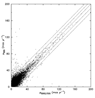
Figure 4: Comparison of the proper motions derived in this study ($\mu_{\rm SDSS/SSS}$) with those from the SuperCOSMOS Sky Survey ($\mu_{\rm SSS}$) in NGS fields 1424 and 1440. Some $\sim$99% of stars fall within the 2$\sigma$ boundaries of a perfect correlation, and the linear correlation coefficient is 0.85. The lack of stars along the $\mu_{\rm SDSS/SSS}$ axis shows close agreement between the SDSS/SSS measures and the corresponding SSS estimates for stars with high SDSS/SSS proper motions, demonstrating the good reliability and negligible contamination of our high proper motion sample.

4.6 The high proper motion sample

4.6.1 Image quality criteria

Prior to the proper motion cut being applied, the data are subject to criteria to ensure that only objects with stellar and high quality images are included in the final sample. From the SSS data the following characteristics of each image are restricted (see Hambly et al. 2001a for more details):

• Blend: Objects appearing as blended in the SSS database are rejected.

• Profile Classification Statistic, $\eta$: This quantifies the ‘stellarness’ of an object by comparing the residuals of the areal profile of an image with that of an average stellar template. Objects with $\eta\geq 4\sigma$ are rejected.

• Quality: During processing the SSS data are assigned a quality flag, which is affected by circumstances such as an image being very large, bright, fragmented or close to a bright star or plate boundary. Images with a quality value of greater than 127 are rejected.

• Ellipticity: The ellipticity of an image is calculated from the weighted semi-minor and semi-major axes given by the SSS processing. Only objects with e $\leq$ 0.25 are included in the sample.

4.6.2 Proper motion selection

A lower proper motion limit is applied to the sample of paired stars for two principal reasons: to amplify the proportion of spheroid stars selected and to create a ‘cleaner’ proper motion sample. The proper motion selection magnifies the contribution from the higher-velocity spheroid population, since they are effectively sampled over larger volumes than the lower-velocity disc stars (Reid, 1997; Cooke & Reid, 2000). The number of stars of each population in a proper motion selected sample is proportional to the mean population tangential velocity:

$$N(\mu>\mu_{min})\propto\rho_{0}\left<V_{T}\right>^{3},$$ (1)

with $\rho_{0}$ the local space density of the population (Hanson, 1983; Reid, 1984). This therefore amplifies the contribution of the higher velocity population above the ratio of the local space densities by the amount:

$$A_{\mu}=\left(\frac{\left<V_{T}^{1}\right>}{\left<V_{T}^{2}\right>}\right)^{3}.$$ (2)

This amplification has a dramatic effect on the likelihood of high velocity stars entering the proper motion sample, and demonstrates the efficiency of proper motion selection in selecting spheroid stars. As seen in Cooke & Reid (2000), a spheroid to disc number ratio of $N_{disc}$:$N_{spheroid}$ = 400:1 for a volume-limited sample can be increased to $N_{disc}$:$N_{spheroid}$ = 5:1 for a proper motion sample.

The second effect of applying a minimum proper motion limit to the sample is to include stars with small relative errors in proper motion, avoiding those with marginal proper motions arising from errors in the positions or pairing. This results in a ‘cleaner’ reduced proper motion diagram (Section 5.1), and a more accurate subdwarf selection.

The lower proper motion limit can be applied either on a global basis, with one limit for all fields, or for each field individually, using the proper motion error estimates from the quasar positions in each field (Section 4.5). Initially this latter approach was used, but evidence of systematic differences between the proper motion accuracies derived for the SGS and NGS led to the adoption of a global proper motion minimum for the entire SGS and NGS sample. The rms of the quasar ‘proper motions’ in each stripe was found to be $\sigma_{\mu}\approx 6.7$ mas yr^-1 for the SGS and $\sigma_{\mu}\approx 8.1$ mas yr^-1 for the NGS. In order to avoid the low proper motion ‘tail’ in each stripe the more conservative value of the NGS error was used for all fields. A 5$\sigma_{\mu}$ cut on the proper motions was applied in defining the lower limit, so that the value used for the entire sample was:

$$\rm\mu_{min}=40.5\ mas\ yr^{-1}.$$ (3)

A maximum proper motion limit is also adopted so as to ensure sample completeness. This limit is theoretically determined by the maximum pairing radius of 10 arcsec, corresponding to $\rm{\mu_{max}\approx 220\ mas\ yr^{-1}}$. However, the actual maximum is somewhat smaller than this value due to systematic shifts in position affecting the pairing process; we therefore adopt a conservative $\rm{\mu_{max}=160\ mas\ yr^{-1}}$ from proper motion number counts (see Section 5.6.1.)

Figure 5 shows the relative proportions of high proper motion stars with $\mu_{min}\la\mu\la\mu_{max}$ in the SGS and NGS. Although there are discrepancies at the bright and faint ends, over the magnitude range of the sample selected (15 $\la r^{*}\la$ 19) the fraction of stars passing the proper motion criteria agree to within a few percent.

Figure 5: The numbers of high proper motion stars in the SGS (solid line) and NGS (dashed line), expressed as a fraction of the total number of paired stars and plotted as a function of magnitude. For the magnitude range of the sample (between the dotted lines) the proportion in each stripe agree to within a few percent, indicating no systematic errors in the derivation of proper motions or high proper motion selection.

5 Methods: the subdwarf sample

5.1 Reduced proper motion

Although applying a lower proper motion limit produces a cleaner sample of fast-moving stars, this will consist not only of subdwarfs but also white dwarfs and high velocity members of the disc. In order to identify the candidate subdwarfs, the reduced proper motion of each star is used as a discriminator. Defined as

$$H=m+5\log\mu+5=M+5\log V_{T}-3.379,$$ (4)

this parameter separates effectively high-velocity (V_T), low-luminosity (M) subdwarfs from the white dwarf and thin disc populations. This is seen in the reduced proper motion diagram (RPMD) of H${}_{r^{*}}$ plotted against $(r^{*}-i^{*})$: Figures 6 and 7 show the RPMDs for all stars with $\mu>\mu_{min}$ in the SGS and NGS respectively. The fainter and higher tangential velocity subdwarfs form a distinct sequence below the thin disc main sequence, whilst the white dwarfs populate the bluest part of the diagram.

The colour index $(r^{*}-i^{*})$ was chosen because of its effectiveness at separating subdwarfs from higher-metallicity stars on colour-magnitude diagrams, due to their lower opacities and higher temperatures at a given mass and luminosity resulting in a larger proportion of their flux being emitted at optical wavelengths (Gizis, 1997; Gizis & Reid, 1999). The $(r^{*}-i^{*})$ index is a good temperature/spectral type indicator for the M dwarfs which dominate this survey (see Section 5.5.1; Lenz et al. 1998; Hawley et al. 2002), so on a reduced proper motion or colour-magnitude diagram it enables clear distinction between the solar-metallicity stars and the hotter (bluer) subdwarfs at each absolute magnitude. The $(r^{*}-i^{*})$ colour is similar to $(R-I_{C})$, proven to be effective at separating subdwarfs in this manner, and covers the TiO and CaH spectral features important for subdwarf classification (Gizis, 1997; Gizis & Reid, 1999). We investigated other appropriate SDSS indices for use in the RPMD, but $(r^{*}-i^{*})$ proved to be the most effective for subdwarf identification.

5.2 Reddening and extinction

With all the fields at high Galactic latitudes ($|b|\geq 37\degr$), interstellar extinction and reddening are unlikely to have a significant impact on this study. To confirm this we use the high-resolution COBE/DIRBE dust maps of Schlegel et al. (1998) to estimate the reddening and extinction at each field centre, using the given wavelength coefficients to convert $E_{B-V}$ and $A_{V}$ to $E_{r^{*}-i^{*}}$ and $A_{r^{*}}$. We find that the majority (23 out of 28) of the SGS and NGS fields have $E_{r^{*}-i^{*}}<0.04$, and that the overall mean is $E_{r^{*}-i^{*}}=0.03$. The maximum reddening is $E_{r^{*}-i^{*}}=0.08$ (for field 0932), and only three fields have $E_{r^{*}-i^{*}}\geq 0.05$, two of which are narrow fields at the end of a stripe and hence contain only a small fraction of the total sample. In applying these estimates we assume that there is no differential reddening across the fields, and that all obscuration is in the foreground. This assumption is valid for our study, since the reddening layer scale height is $\sim$100 pc (Chen et al., 1999), and our survey is sensitive to very few stars within this distance (see Section 5.5.2.)

With photometric accuracy of $\sim$3% in the $r^{*}$ and $i^{*}$ bands of the EDR (Stoughton et al., 2002), the size of the reddening effect is comparable to that of the $\sigma_{r^{*}-i^{*}}\approx 0.04$ colour errors. Inspection of the reduced proper motion diagrams (Figures 6 and 7) shows that adjustments of this order would have little effect on the “tightness” of the population locii and subsequent subdwarf selection. The mean extinction over all fields is $A_{r}=0.126$, which if not corrected for would result in derived photometric parallaxes being underestimated by up to $\sim$5%, less than the expected distance errors. These considerations suggest that the effects of reddening and extinction on the study are negligible, and so corrections are not applied to the data.

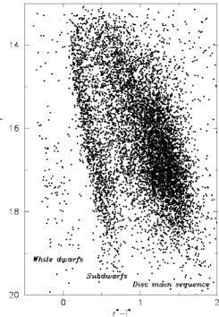
Figure 6: The RPMD for stars with $\mu\geq\mu_{\rm{min}}$ in the SGS. The three separate sequences of white dwarfs, subdwarfs and thin disc stars are clear.

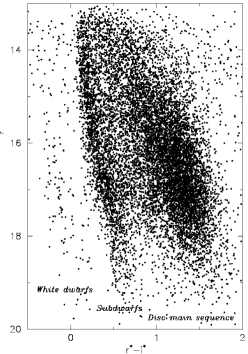
Figure 7: The RPMD for stars with $\mu\geq\mu_{\rm{min}}$ in the NGS.

5.3 Tangential velocity cut-off

Although the RPMD separates the subdwarfs from the thin disc stars and white dwarfs, there is some overlap on the diagram with the locus of thick disc stars. These have relatively high velocities, and hence are responsible for the objects lying between the old disc and subdwarf sequences. Thick disc stars have a much higher local number density than subdwarfs, and the inclusion of even a tiny proportion of this population in the sample can result in a significant overestimation of the spheroid density (Bahcall & Casertano, 1986).

However, the contamination of the sample by these stars can be avoided by the introduction of a cut-off in tangential velocity. Figure 8 shows calculated tangential velocity distributions of the disc and spheroid populations in the direction of one of the SGS fields, assuming a velocity ellipsoid described by a solar motion and Gaussian dispersions (Table 3) and following the method given in Murray (1983, p285).

For our assumed velocity ellipsoids we adopt the disc kinematics derived from two analyses of local M dwarfs (Reid, Hawley & Gizis, 1995; Hawley, Gizis & Reid, 1996), and the spheroid ellipsoid derived from the study of a large sample of low metallicity stars by Chiba & Beers (2000). The parameters of these ellipsoids are given in Table 3.

It is clear that a limit of $V_{T}>$ 200 km s^-1 will exclude all but a negligible proportion of the thick disc population: our calculations suggest that a maximum of just 0.04% of the thick disc population will be included in such a sample. This cut-off will also cause the low-velocity tail of the spheroid population to be excluded from the sample, but our calculation results allow us to correspondingly correct the derived luminosity functions (see Section 6.4.)

Figure 8: Simulated tangential velocity distributions for the thin and thick disc and spheroid (in order of increasing velocity) in the direction of field 0363 in the SGS

Table 3: Adopted velocity ellipsoids. The assumed disc (Reid et al. 1995; Hawley et al. 1996) and spheroid (Chiba & Beers, 2000) stellar kinematics used in the tangential velocity calculations. All speeds are in kms^-1, and U, V, W denote the usual Galactic coordinate triad in the respective directions of the Galactic center, direction of rotation and NGP.

Population	U☉	V☉	W☉	$\sigma_{U}$	$\sigma_{V}$	$\sigma_{W}$
Spheroid	-26	-199	-12	141	106	94
Thin Disc	10	-5	-7	41	27	21
Thick Disc	10	-23	-7	52	45	32

5.4 Selecting candidate subdwarfs

5.4.1 The colour-magnitude relations

Equation (4) suggests that with an assumed colour-magnitude relation, lines of constant $V_{T}$ can be plotted on the RPMD. A spheroid-disc separating line of $V_{T}$ = 200 km s^-1 can then be applied to the RPMD in order to select candidate subdwarfs, with an upper RPM limit used to exclude white dwarfs from the sample. An accurate colour magnitude relation is also required to derive photometric parallaxes for each star in the sample, necessary for computation of the luminosity function.

Obtaining a reliable colour-magnitude relation for subdwarf stars empirically is problematic, due to the existence of relatively few known subdwarfs with accurate trigonometric parallaxes. Theoretical relations derived from model atmospheres exist as an alternative (Baraffe et al., 1997), and these provide excellent matches to cluster sequences and closely follow the majority of field star data, especially in the infrared (Baraffe et al., 1997, 1998; Chabrier, 2003). However, the metal-rich versions ([m/H] $\ga-1.0$) of these models suffer from discrepancies with the lower end of the observed main sequence ($V-I_{C}\ga 2.0$) in optical colours (Baraffe et al., 1998; Chabrier, 2003). Whilst lower-metallicity models are expected to be less affected in this way, when matched to field stars they still yield poor reproductions of the observed colours at redder wavelengths (Baraffe et al., 1997; Chabrier, 2003), and exhibit possible systematic errors in metallicity when used to estimate abundances from colour-magnitude diagrams (Gizis, 1997; Gould et al., 1998). These factors could significantly affect the ability of the models to provide the reliable optical colour-magnitude relations required here, calculating an expected absolute magnitude for each subdwarf given an observed colour and metallicity estimate. Therefore, whilst the latest theoretical model atmospheres provide good matches to most of the stellar physics and observed parameters, the possibility of systematic colour offsets, perhaps wavelength-dependent, leads us to choose to employ an empirical colour-magnitude relation for this study.

An obstacle in applying a colour-magnitude relation to halo stars is the large range of metallicities present in the spheroid, and hence the spread of absolute magnitude for a given colour. Without spectra to obtain metallicities we deal with this degeneracy in two ways: by using one approximate colour magnitude relation for selecting subdwarfs on the RPMD, and a more accurate estimate which predicts metallicity from observed colours for deriving photometric parallaxes.

5.4.2 The colour-magnitude relation for selecting subdwarfs

The colour-magnitude relation used to select subdwarfs from the RPMD is obtained in a similar way to that of Gizis & Reid (1999). We derive separate relations for low and high metallicity subdwarfs, following the classifications defined by Gizis (1997) of stars with [Fe/H] $\approx-1.2\pm$0.3 as subwarfs (sd), and with [Fe/H] $\approx-2.0\pm$0.5 as extreme subwarfs (esd).

To derive a colour-magnitude relation we use calibrating subdwarfs from the compilations of Gizis (1997) and Reid et al. (2001). Both of these studies use the spectral classification scheme described in Gizis (1997) to identify subdwarfs, and give accurate trigonometric parallaxes for their samples. These are derived principally from the USNO (Monet et al., 1992) and Yale (4th ed; van Altena et al. 1995) catalogues in the case of Gizis, and from the Hipparcos catalogue (Perryman et al., 1997) in the case of Reid et al. (2001).

We consider only subdwarfs with $\sigma_{\pi}/\pi<$0.2 so as to ensure accuracy of the absolute magnitudes, producing a total of 35 subdwarfs and extreme subdwarfs from Gizis, and 38 from Reid et al. We plot these stars on a M_I, $(V-I_{\rm C}$) Hertzsprung-Russell diagram (Johnson $V$ and Cousins $I_{\rm C}$), and fit a colour-magnitude relation to the sdM and esdM separately. Stellar colour-magnitude relations are poorly matched by a linear relation due to an inflection in the subdwarf main sequence at V-$I_{\rm C}\sim$1.5 (Baraffe et al., 1997), so we match a cubic spline to the parallax data (Figure 9.)

Figure 9: Colour-magnitude relations derived from subdwarfs with accurate trigonometric parallaxes. Squares denote subdwarfs and triangles extreme subdwarfs; filled symbols are subdwarfs from Gizis (1997) and open symbols are those from Reid et al. (2001)

There is currently no published SDSS photometry for stars with accurate trigonometric parallaxes, so it is necessary to first derive the colour-magnitude relation in the standard Johnson/Cousins photometric systems, and then convert the colours and magnitudes to SDSS $r^{*}$ and $r^{*}-i^{*}$. This is done by means of the relation

$$M_{r^{*}}=r^{*}-V+(V-I_{\rm C})+M_{I},$$ (5)

combined with two-colour relations to convert from SDSS ($r^{*}-i^{*}$) to ($r^{*}-V$) and ($V-I_{\rm C}$).

These two-colour relations should ideally be obtained from subdwarfs with accurate photometry and similar metallicities to those in our sample. However, of the subdwarfs in the SDSS Standard Star Catalogue (Smith et al., 2002), very few have published $VI_{\rm C}$ photometry and span only a small range in colour. We therefore fit linear two-colour relations between the Johnson/Cousins and SDSS systems for higher-metallicity disc stars instead. Despite this, applying these fits to the few subdwarf stars with SDSS and $VI_{\rm C}$ magnitudes suggests that the disc metallicity fits apply well to the spheroid metallicity stars. The relations derived are

$$r^{*}-V=-0.889(r^{*}-i^{*})-0.040,$$ (6)

$$V-I_{\rm C}=2.097(r^{*}-i^{*})+0.429,$$ (7)

and are shown in Figure 10.

Figure 10: Two-colour relations from the SDSS to Johnson/Cousins photometric systems for disc stars in the SDSS standard star catalogue. There is little to suggest that these relations are strongly dependent on metallicity.

5.4.3 Selecting candidate subdwarfs

With an approximate colour-magnitude relation with which to estimate M${}_{r^{*}}$ given ($r^{*}-i^{*}$) for an assumed subdwarf, we can make use of Equation (4) to plot lines of constant $V_{\rm T}$ on the RPMD.

Figure 11 shows the RPMD for the high proper motion stars in one of our fields (POSS-I field 0465 in the NGS), with the lines corresponding to 200 and 500 km s^-1 that we use to identify our candidate subdwarfs. These limits clearly provide a good match to the observed subdwarf sequence, and are applied on a field-by-field basis to account for the varying kinematics between fields. The lower velocity bound is applied to avoid contamination from thick disc stars, whereas the upper limit is applied to prevent selection of white dwarfs. With knowledge of the expected tangential velocity distributions for the disc and spheroid stellar populations (Section  5.3) we can estimate the fraction of spheroid and thick disc stars that are expected to fall within this velocity range to compensate for selection effects (Section 6.4). The numbers of high proper motion stars and subdwarfs passing all selection criteria (including metallicity constraints for subdwarfs) are shown in Table 4.

Table 4: The numbers of high proper motion stars $(N_{hpm})$ and subdwarfs $(N_{sd})$ passing all magnitude, proper motion, quality and metallicity selection criteria for each field.

SGS                                NGS
Field $N_{hpm}$ $N_{sd}$ 0932 296 15 0363 757 68 1453 703 81 1283 747 85 0852 709 80 0362 814 91 1259 804 89 1196 790 107 0591 875 96 0319 864 84 0431 847 90 0834 320 32 Total: 8526 918 Field $N_{hpm}$ $N_{sd}$ 0151 256 44 1402 703 143 1613 700 125 1440 814 145 1424 866 145 0465 910 164 1595 853 130 1578 802 128 1405 947 125 1401 1005 125 0471 947 111 1400 813 89 1397 704 69 0467 762 76 0470 600 56 1318 282 21 Total: 11964 1696

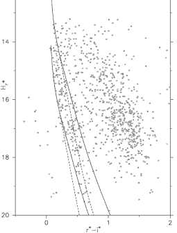
Figure 11: The RPMD for high proper motion stars in NGS field 0465, with the subdwarf (solid lines) and extreme subdwarf (dashed lines) selection lines corresponding to V_T = 200 and 500 kms^-1 overlaid.

5.5 Metallicities and photometric parallaxes

5.5.1 Estimating metallicities

The division of the subdwarf colour-magnitude relation into two metallicity ranges is clearly a poor approximation, and one that is unsuitable for use in obtaining photometric parallaxes of the candidate stars. The spread of nearly two magnitudes in luminosity between metal-rich and metal-poor subdwarfs at $(V-I_{\rm C})\approx$ 2 could lead to significant errors in the distance estimates, so a more robust method which accounts for the absolute magnitude-metallicity degeneracy is required.

The highly accurate five band photometry of the SDSS is ideally suited for estimating metallicities from colours. The photometric precision is sufficient to clearly separate stars of differing metallicities when plotted in metallicity-sensitive colours such as ($u^{*}-g^{*})$ and $(g^{*}-r^{*})$ (Figure 13). We use all five photometric bands matched to model atmosphere grids in order to derive a metallicity estimate for each subdwarf candidate.

The model atmospheres of Lenz et al. (1998) use Kurucz ATLAS9 models (Kurucz, 1993) to give grids of four synthetic SDSS colours for stars with effective temperatures ($T_{eff}$) from 3500 to $40\,000$ K and varying metallicity and $\log g$. Adopting a value of $\log g$ = 4.5 and given the observed colours, we use a chi-square statistic and interpolate in the grids to estimate the best-fit temperature and metallicity for each subdwarf. Stars with poor metallicity-temperature fits are eliminated by rejecting all candidates with a residual greater than twenty times the rms value of the residuals of the grid fit. This leads to some 3% of candidates being rejected, although their highly unusual colours means that most of these objects will not be subdwarfs.

It is clear from inspection of the metallicities derived that there is a zero point error in the estimates, with the median metallicity for each stripe of $\widetilde{[m/H]}\sim-2.4$ considerably lower than the [Fe/H]$\sim-1.5$ expected for spheroid stars (Laird et al., 1988; Nissen & Schuster, 1991). There are a number of likely contributing causes of this: one is that the [m/H] = $-5.0$ model only extends blueward of $(g^{*}-r^{*})\approx 0.7$, and so the metallicities of subdwarfs redder than this have to be extrapolated from the [m/H]$\geq-2.0$ models. Even subdwarfs with $(g^{*}-r^{*})\la 0.7$ rely on interpolation between the [m/H]$=-5.0$ and $-2.0$ models – a very large metallicity spread which will inevitably introduce errors. Additionally, inaccuracies in the model atmospheres will lead to uncertainties in the derived metallicities, particularly for redder stars. However, the observed offset is largely irrelevant to this application as we are interested in only the relative metallicities of the sample. Aside from the zero point error, the derived metallicities and temperatures show good consistency, both with the expected correlations on a temperature-colour diagram (Figure 12) and in colour-colour plots (Figure 13). Additionally, the metallicity distributions of both the SGS and NGS are in close agreement (Figure 14), indicating no significant systematic difference (whether intrinsic or not) between the samples.

Figure 12: The correlation between effective temperature and $r^{*}-i^{*}$, with model predictions for [m/H] = $-1.0,-2.0,-5.0$ (in order of increasing temperature at $r^{*}-i^{*}\sim 0.2$) from Lenz et al. (1998). For the majority of stars (those with $r^{*}-i^{*}\la 0.4$) there is close agreement with the models and good internal consistency of the metallicity and temperature estimates. The poor fit of the models for $r^{*}-i^{*}\ga 0.4$ is likely to be mostly due to less accurate temperature interpolations over this range, arising from the larger colour spread and the fact that the [m/H] = $-5.0$ model does not extend to these redder wavelengths. However, since the majority of the sample lies blueward of $r^{*}-i^{*}\approx 0.5$ and the metallicities are not used in an absolute sense, the effect of these discrepancies will be limited.

Figure 13: Colour-colour plots for subdwarfs in the SGS (top) and NGS (bottom), with model atmosphere predictions for stars of [m/H] = $+1.0,0.0,-1.0,-2.0$ and $-5.0$ (from bottom to top) overlaid. There is no evidence for any systematic metallicity difference between the samples.

Figure 14: The estimated metallicity distributions for the SGS (solid line) and NGS (dashed line). Although the metallicities are clearly not accurate in an absolute sense from comparison with the [Fe/H] $\sim-1.5$ expected for spheroid stars, there is good agreement between the samples and no systematic metallicity difference between the two. The median metallicities of $-2.5$ for the SGS and $-2.3$ for the NGS agree well within the expected errors.

5.5.2 Photometric parallaxes

With a metallicity estimate for each candidate subdwarf, a metallicity-dependent colour-magnitude relation is used to provide a more reliable indication of each star’s intrinsic luminosity. A median colour-magnitude relation $\widetilde{M_{I}}$ is derived by fitting a single cubic spline to all the parallax subdwarfs in Section 5.4.2. The absolute magnitude $M_{I}^{*}$ of each star in the sample is then estimated by offsetting from this median magnitude by an amount proportional to the star’s deviation from the sample median metallicity at that particular colour. The estimated absolute magnitude is given by:

$$M_{I}^{*}=\widetilde{M_{I}}+d[m/H]w\frac{dM_{I}}{d[m/H]}\biggr{|}_{(r^{*}-i^{*})},$$ (8)

where

$$d[m/H]=[m/H]^{*}-\widetilde{[m/H]}_{(r^{*}-i^{*})},$$ (9)

is the metallicity offset of the star from the sample median at that colour, $w$ is a weighting function to allow for colour-dependent errors, and the derivative is the variation of absolute magnitude with metallicity derived from theoretical colour-magnitude relations.

The weight function corrects for the larger colour and metallicity errors at redder wavelengths by assigning a weight relative to the metallicity spread at each particular colour. Hence

$$w=\left(\frac{\sigma_{[m/H]}^{true}}{\sigma_{[m/H]}}\right)^{2},$$ (10)

where $\sigma_{[m/H]}^{true}$ is the assumed intrinsic metallicity spread, given by the rms metallicity deviation from the median for 0.1 $\leq(r^{*}-i^{*})\leq$ 0.25, and $\sigma_{[m/H]}$ is the rms metallicity spread at a given colour. This weighting therefore assumes that the metallicity range for the sample is independent of colour.

The derivative of absolute magnitude with respect to metallicity at each colour is derived from the theoretical colour-magnitude relations for stars of different metallicities provided by Baraffe et al. (1997). The metallicity-absolute magnitude relation varies considerably with colour (Figure 15), but is approximately linear. The slope of this relation is therefore a constant and is estimated from the models for each star’s colour to provide the last term in Equation (8). The models of Baraffe et al. (1997) and the parallax subdwarfs are given in the $(M_{I},V-I_{C})$ colour plane; conversion to SDSS colours is achieved using Equation (5).

Figure 15: The correlation of absolute magnitude with metallicity from the models of Baraffe et al. (1997), for $(V-I_{C})$ from 1.0 (top) to 2.8 (bottom) in steps of 0.2.

It is stressed that this modification of the colour magnitude relation based upon estimated metallicity is only an approximation. It is only intended to adjust the predicted magnitude of each star according to its likely metallicity in the right direction and by roughly the right amount. In light of this the adjustment of absolute magnitude from the median is restricted to a maximum of $\pm$1.5 mag, to prevent any stars being assigned inappropriate values. However, it can be seen from the sample estimated colour-magnitude diagram (Figure 16) that this method provides a far more realistic and accurate distribution of absolute magnitudes than a simple division of the colour-magnitude relation into two metallicity ranges.

Figure 16: Estimated absolute magnitudes for all subdwarfs in the SGS and NGS, derived from a median colour-magnitude relation fitted to calibrating subdwarfs (solid line) and offset according to the metallicity estimate of each star.

With an estimated absolute magnitude for each star a distance can then be derived, assuming no significant reddening effects due to the high latitude of the fields ($|b|\geq 37\degr$). The distances sampled are in the range $\sim$260 pc to $\sim$2.8 kpc, and the distributions for the SGS and NGS are shown in Figure 17. That proportionally fewer stars with distances over 2 kpc are found in the SGS compared to the NGS is an effect expected in a non-uniform spheroid density distribution. Whereas the NGS is directed principally towards the inner quadrants of the Galaxy, the SGS lies towards the outer quadrants where the space density of stars will be lower with a non-uniform distribution.

Figure 17: The distributions of estimated distances for the SGS (top) and NGS (bottom).

5.6 Tests for sample systematic errors

The luminosity functions derived from the two independent SGS and NGS samples not only provide an excellent probe of the spheroid density distribution, but also can be compared to ensure that our results are free from significant systematic errors – a source of concern with earlier studies (Section 2).

Prior to comparing the results from each stripe, however, we must ensure that the two samples are self-consistent and free from systematic effects. Inconsistency between the samples could arise from either a systematic disparity in the selection of each sample, or from an intrinsic difference in the constituent stars of each.

5.6.1 Sampling systematic errors

Systematic errors arising from the sample selection are the most likely, with a whole range of possible causes such as a difference in astrometric or photometric accuracy between the stripes. However, we can test for any significant difference of this type by investigating the completeness of each subdwarf sample. We do this in a somewhat crude manner by comparing cumulative proper motion number counts: assuming a uniform stellar density and that proper motion and distance are inversely proportional ($\mu\propto d^{-1}$), a plot of log cumulative number count ($\Sigma N$) against $\log\mu$ should have a gradient of $-3$:

$$\Sigma N\propto V\propto d^{3}\propto\mu^{-3}.$$ (11)

Figure 18 shows the histogram of cumulative proper motion counts for all paired stars in the NGS and SGS after the error mapper has been applied. We fit a straight line to the points between the global proper motion limits for each stripe: $\mu_{\rm{min}}$ = 40.5 mas yr^-1 and $\mu_{\rm{max}}$ = 160 mas yr^-1. Both give a close fit to the expected gradient: $-2.92\pm$ 0.06 for the SGS and $-2.99\pm$ 0.06 for the NGS. Similar plots for just the candidate subdwarfs in each stripe are shown in Figure 19, where gradients of $-3.10$ are found for each stripe.

There is some evidence for incompleteness in the non-linearity of the histograms, especially for the subdwarf samples where proper motion errors lead to incompleteness towards the proper motion limits. This is particularly relevant to the higher proper motions where the errors will be more dominant, and this explains the rapid tailing off of the distributions for $\log\mu\ga$ 2.1 caused by the imposition of the upper proper motion limit. However, the number counts for the population from which the subdwarfs are selected (Figure  18) demonstrate that it is complete for 40.5 mas yr^-1$\leq\mu\leq$ 160 mas yr^-1, and the good match of all of the histograms to the expected gradient of $-3$ indicate that there are no significant signs of incompleteness affecting the samples. It must be also stressed that these are only approximate tests for completeness, and will have some unreliability introduced by the assumption of uniform stellar density, which is particularly invalid for stars at large distances which tend to have lower proper motions.

Figure 18: Cumulative proper motion number counts for all stars in the SGS (top) and NGS (bottom). The straight line fits between the proper motion limits in each stripe are shown (dashed line), along with the expected line of gradient of $-3.0$ (dotted line).

Figure 19: Cumulative proper motion number counts for candidate subdwarfs in the SGS (lower line) and NGS (upper line). The straight line fits between $1.6\leq\log\mu\leq$ 2.1 (dashed lines) both have gradients of $-3.1$

5.6.2 Radial metallicity gradient

An intrinsic difference between the samples that could have a significant effect on the results is a difference in median metallicity between the SGS and NGS. Although the radial metallicity gradient of the inner spheroid is thought to be small ($\Delta[Fe/H]/\Delta r\approx-0.012$ dex kpc^-1, Bekki & Chiba 2001), with both samples in opposite radial Galactic directions this could nevertheless introduce a source of error. The assumption of a single colour-magnitude relation for both of the samples would mean that stars in the sample with the higher metallicity would have their absolute magnitudes overestimated, and hence their distances and contribution to the luminosity function would be underestimated. The derived luminosity function of each sample would therefore be expected to differ. This effect would be less pronounced with the photometric parallax relation defined in Section 5.5.2 that partially accounts for metallicity variations, but is an issue that should still be addressed.

However, our data display little evidence of metallicity gradient. The two-colour diagrams for the subdwarf sample in each stripe in Figure 13 show no systematic difference, and the estimated metallicity distribution and median metallicity of each (Figure 14) are very similar. It is therefore highly unlikely that there is any strong systematic metallicity difference between the samples.

These checks of sample consistency indicate that there are no large systematic differences between the samples arising from sampling errors or intrinsic variations. A further and final test of the sample completenesses can be ascertained following the luminosity function calculations from the value of $\langle V/V_{\rm max}\rangle$ (Section 7).

6 Methods: The luminosity function

6.1 The generalised $\mn@boldsymbol{V_{max}}$ method

With a final sample size of 918 candidate subdwarfs in the SGS and 1696 in the NGS, the luminosity function can be accurately derived. We achieve this using a modification of the $V_{max}$ method of Schmidt (1968): each star contributes 1/$V_{max}$ to the luminosity function, where $V_{max}$ is the maximum volume that the star could have been detected in, given the proper motion and magnitude limits of the survey. This technique therefore implicitly corrects for any bias arising from the proper motion selection.

Schmidt’s original 1/$V_{max}$ method assumes that the sample is selected from a uniformly-distributed population. This certainly is not the case for our subdwarf sample; indeed, we intend to use it to determine the variation in spheroid density. We therefore adopt the ‘generalised $V_{max}$’ method (Stobie, Ishida, & Peacock, 1989; Tinney, Reid, & Mould, 1993), which extends Schmidt’s method to non-uniformly distributed samples. Given that each star in the survey can be detected to minimum and maximum distances ${d_{min},d_{max}}$ in a field of solid angle $\Omega$, the luminosity function is defined as:

$$\rm{\Phi_{sample}=\sum\frac{1}{V_{max}^{{}^{\prime}}}},$$ (12)

$${V_{max}^{{}^{\prime}}}=\Omega\int^{d_{max}}_{d_{min}}s^{2}\frac{n(s)}{n_{\odot}}\ ds,$$ (13)

where $s$ is the heliocentric distance and $n(s)$ is the adopted spheroid density law (Section 6.3).

6.2 Proper motion and magnitude limits

The distance limits depend on the minimum and maximum proper motion and magnitudes in each field. The upper and lower proper motion limits employed are $\mu_{min}=40.5$ mas yr^-1 and $\mu_{max}=160$ mas yr^-1 (Section 4.6.2).

Ascertaining the magnitude limits for each field is less straightforward as the data come from two quite different sources, and there is significant variation in the depth of the plate material. However, the fact that the datasets are paired and that the SDSS data probe much fainter ($r^{*}\sim$ 23) than the POSS-I plates means that only the $r^{*}$ magnitudes need be considered.

The POSS-I plates reach incomplete levels at R $\sim$ 20, at which magnitude the SDSS data are certainly complete. Stars need to appear in both datasets to pass the pairing criteria, so the faint magnitude limit can be defined solely in terms of the much more accurate SDSS $r^{*}$ magnitude. A (log number, $r^{*}$ magnitude) histogram is plotted for all of the paired stars in each field, and an upper limit is conservatively defined from the magnitude at which $\log\left(N\left(r^{*}\right)\right)$ departs from a steady increase (Figure 20; Table 5.) The brighter limit is less crucial due to the smaller likelihood of subdwarfs having such magnitudes, but a limit of $r^{*}\sim 15$ is applied to encompass the range that is likely to be complete as indicated by the histogram.

Figure 20: The log number - magnitude histogram for all unpaired (top) and paired (bottom) stars in the NGS, with the approximate upper and lower $r^{*}$ magnitude limits for the NGS fields shown. The actual magnitude limits adopted for each field are ascertained from where the $\log(N(r^{*}))$ curve in the field’s histogram departs from a steady increase.

Table 5: Magnitude limits and spheroid and thick disc discovery fractions for SGS (top) and NGS (bottom) fields. The minimum magnitude limit for all fields is $r^{*}$ = 15.0 and the proper motion limits are $\mu_{min}=40.5$ mas yr^-1 and $\mu_{max}=160$ mas yr^-1.

Field	$r^{*}_{max}$	$\chi_{h}$(%)	$\chi_{td}(\%)$
0932	18.7	61.15	0.01
0363	19.5	62.56	0.01
1453	19.0	63.57	0.01
1283	19.2	64.16	0.02
0852	19.1	64.39	0.02
0362	19.2	64.27	0.02
1259	19.1	63.85	0.03
1196	19.1	63.13	0.03
0591	19.3	62.13	0.04
0319	19.2	60.85	0.04
0431	19.0	59.31	0.04
0834	18.9	57.50	0.04
0151	19.0	61.15	0.01
1402	19.2	62.56	0.01
1613	18.8	63.57	0.01
1440	19.1	64.16	0.02
1424	19.1	64.39	0.02
0465	19.0	64.27	0.02
1595	18.7	63.87	0.03
1578	18.9	63.13	0.03
1405	19.0	62.12	0.04
1401	19.2	60.85	0.04
0471	19.2	59.31	0.04
1400	19.0	57.50	0.04
1397	18.7	55.42	0.03
0467	19.3	53.26	0.03
0470	19.1	50.94	0.03
1318	18.8	48.62	0.03

With proper motion limits $\mu_{\rm{min}}$, $\mu_{\rm{max}}$ and magnitude limits $r_{\rm{min}}^{*}$, $r_{\rm{max}}^{*}$ for each field, the limiting distances for a subdwarf of distance $d$ and magnitude $r^{*}$ are therefore defined as

$$\ d_{\rm{min}}=d\ \rm{max}\left[\frac{\mu}{\mu_{max}},10^{0.2\left(r_{min}^{*}-r^{*}\right)}\right],$$ (14)

$$d_{\rm{max}}=d\ \rm{min}\left[\frac{\mu}{\mu_{min}},10^{0.2\left(r_{max}^{*}-r^{*}\right)}\right].$$ (15)

6.3 The spheroid density law

Recent studies of the structure of the Galactic spheroid have indicated that its density profile is flattened and follows a power law: an axial ratio of (c/a)$\approx$ 0.6 and $\rho(r)\sim r^{-3}$ (Gould et al., 1998; Sluis & Arnold, 1998; Yanny et al., 2000; Ivezić et al., 2000; Chen et al., 2001; Siegel et al., 2002; Gould, 2003). We therefore adopt a spheroid density law of the form

$$\frac{n}{n_{\odot}}=\left(\frac{r_{c}^{2}+R_{0}^{2}}{r_{c}^{2}+R^{2}+z^{2}/q^{2}}\right)^{\alpha},$$ (16)

where $n_{\odot}$ is the local spheroid density, $\alpha$ is the power law index and $q=(c/a)$ is the axial ratio, and we assume $R_{0}$ = 8.0 kpc and $r_{c}$ = 1.0 kpc. Converting the Galactocentric cylindrical coordinates $R$ and $z$ in terms of heliocentric coordinates $(s,l,b)$, where $s$ is the distance from the Sun and $l$ and $b$ are Galactic latitude and longitude:

$$\frac{n}{n_{\odot}}=\left(\frac{r_{c}^{2}+R_{0}^{2}}{r_{c}^{2}+R_{0}^{2}+s^{2}-2sR_{0}\cos l\cos b+s^{2}\sin^{2}b\frac{1-q^{2}}{q^{2}}}\right)^{\alpha}.$$ (17)

The two density law parameters $\alpha$ and $q$ are allowed to vary, and luminosity functions are derived for a range of values to find the $(\alpha,q)$ law which best matches the observations (see Section 6.8.) A significant benefit of this approach is that the density law variables $\alpha$ and $q$ can be fitted without having to make an assumption about the local spheroid density $n_{\odot}$.

6.4 Discovery fraction

Given distance limits and an assumed $(\alpha,q)$ density distribution, the sample luminosity function can then be calculated. However, the tangential velocity cut-offs cause the sample to exclude a given fraction of spheroid stars, so this scaling needs to be taken into account in order to derive the true spheroid luminosity function from the sample.

The fraction $\chi_{h}$ of spheroid stars expected to have 200 km s${}^{-1}\leq V_{T}\leq$ 500 km s^-1 is calculated for each field using tangential velocity calculations as described in Section 5.3. Using our adopted velocity ellipsoids, $\chi_{h}$ varies between 0.58 and 0.64 in the SGS, and 0.49 and 0.64 in the NGS (Table 5), and scales the spheroid luminosity function as

$$\rm\Phi_{h}^{true}=\frac{1}{\chi_{h}}\Phi_{h}^{sample}.$$ (18)

At this stage any possible contamination by thick disc stars can be considered. Assuming they are also included in the sample with $V_{T}\geq 200$km s^-1, then the derived luminosity function will comprise a total for spheroid and thick disc members. The sample spheroid luminosity function can then be calculated from the total (spheroid plus thick disc) by

$$\rm\Phi_{h}^{sample}=\lambda_{h}\Phi_{h+td}^{sample},$$ (19)

where $\lambda_{h}$ is the fraction of spheroid stars in the sample. This is given by

$$\lambda_{h}=\frac{1}{(\chi_{td}\left/\chi_{h}\right.)(n_{td}\left/n_{h}\right.)+1},$$ (20)

where $\chi_{td}$ and $\chi_{h}$ are the fractions of thick disc and spheroid stars with 200km s^-1 $\leq V_{T}\leq$ 500 km s^-1 and $n_{td}$ and $n_{h}$ are the local number densities of thick disc and spheroid stars. The discovery fractions $\chi_{td}$ and $\chi_{h}$ are known from the calculations described in Section 5.3, whilst the relative normalisation of thick disc to spheroid stars is taken from independent studies. Assuming a thick to thin disc density ratio of 1:10 (Reid et al. 1995; Chen, Stoughton & Smith 2001; Siegel et al. 2002) and a combined disc to spheroid normalisation of 400:1 (Chabrier & Mera, 1997; Holmberg & Flynn, 2000), we adopt a thick disc to spheroid ratio of $n_{td}$:$n_{h}$ = 40:1. With this consideration of thick disc contamination, the true spheroid luminosity function is therefore derived from

$$\rm\Phi_{h}^{true}=\frac{\lambda_{h}}{\chi_{h}}\Phi_{h+td}^{sample}.$$ (21)

However, with a tangential velocity cut-off of $V_{T}\geq 200$ km s^-1, this scaling for thick disc contamination has very little effect on the luminosity function. This normalisation gives a scaling factor of $0.97\leq\lambda_{h}\leq 1.00$, so at worst the thick disc contamination has just a three percent effect on the normalisation of the luminosity function.

6.5 Luminosity function errors

In estimating the errors in the luminosity function we adopt the assumption of Poissonian errors (Felten, 1976):

$$\sigma_{\Phi_{\rm sample}}^{2}=\sum{\frac{1}{V_{max}^{2}}}.$$ (22)

Allowing for scaling:

$$\sigma_{\Phi_{\rm true}}^{2}=\left(\frac{\lambda_{h}}{\chi_{h}}\right)^{2}\sigma_{\Phi_{\rm sample}}^{2}.$$ (23)

6.6 Combining fields

Whilst the luminosity functions and densities for each field are derived separately to investigate the spheroid density profile, it is desirable to calculate a combined luminosity function for the fields in each stripe. Unfortunately the necessity of scaling to account for the spheroid discovery fraction and thick disc contamination on a field by field basis means that a total 1/$V_{max}$ luminosity function cannot be calculated for the whole sample. However, a combined luminosity function for all of the fields in each stripe can be derived by combining the luminosity functions for each field with a simple weighted mean. The mean density and error for each magnitude bin are then given by

$$\rm\overline{{\log\Phi}}=\frac{\sum{\log\Phi\left/\sigma_{\log\Phi}^{2}\right.}}{\sum{1\left/\sigma_{\log\Phi}^{2}\right.}},$$ (24)

$$\rm\sigma_{\overline{{\log\Phi}}}^{2}=\frac{1}{\sum{1\left/\sigma_{\log\Phi}^{2}\right.}},$$ (25)

where the summations are over the fields in each stripe.

6.7 Transforming $\Phi(M_{r^{*}})$ to $\Phi(\rm M_{V})$

To facilitate comparison with published luminosity functions, it is necessary to convert the derived luminosity function from SDSS $r^{*}$ absolute magnitude to Johnson $V$. This is achieved using the transformation

$$\Phi\left(M_{V}\right)=\Phi\left(M_{r^{*}}\right)\frac{dM_{r^{*}}}{dM_{V}}.$$ (26)

The derivative is evaluated from

$$M_{V} = M_{r^{*}}-(r^{*}-V)$$ (27)

$$= M_{r^{*}}-\left[(-0.889(r^{*}-i^{*})-0.040\right],$$ (28)

from Equation (6). By varying ($r^{*}-i^{*}$), $M_{r^{*}}$ can be plotted against $M_{V}$, a spline fitted and the derivative evaluated (Figure 21). Hence $dM_{r^{*}}/dM_{V}$ can be calculated for a given $M_{r^{*}}$, and repeating this for each $M_{r^{*}}$ bin in the luminosity function completes the transformation.

Figure 21: The relations between $M_{r^{*}}$ and $M_{V}$ (solid line) and $\frac{dM_{r^{*}}}{dM_{V}}$ (dot-dashed line) derived from the two-colour relations. These are used to convert the luminosity function derived in $M_{r^{*}}$ to $M_{V}$ to facilitate comparison with published results.

6.8 Constraining the spheroid density profile

With a wide range of lines of sight, the SGS and NGS samples are ideally suited to constraining the density distribution of the spheroid. Indeed, a non-uniform density law has to be assumed in order to compare the luminosity functions of the different samples. Figure 22 shows the number densities (luminosity function integrated over 5 $\leq M_{r^{*}}\leq$ 10) for each field plotted against Galactic longitude when derived using a conventional $V_{max}$ method under the assumption of uniform space density. It is clear from comparison with the models that at the distances sampled the varying density of the spheroid has a strong effect and so has to be taken into account when deriving the luminosity function.

In order to constrain the density distribution a power law of the form given in Equation (17) is assumed, and subdwarf number densities are calculated for each field in the SGS and NGS for a range of power law indices and axial ratios. The power law index $\alpha$ is allowed to vary from $-2.0$ to $-4.4$ in steps of 0.05, and the axial ratio from 0.2 to 1.0 in intervals of 0.05.

The generalised $V_{max}$ method (Section 6.1) should ensure that the derived number densities are constant and independent of line of sight, so how well a $(\alpha,q)$ power law model fits the data is ascertained by measuring how close to a uniform value the field number densities are under the model. This goodness of fit is defined by a modified chi-square statistic

$$\chi^{2}=\sum_{i=1}^{nf}\sum_{j=i}^{nf}\frac{\left(n_{i}-n_{j}\right)^{2}}{\sigma_{i}^{2}+\sigma_{j}^{2}},$$ (29)

where $n_{i}$ and $\sigma_{i}$ are the number density and its standard deviation for each of $nf$ fields. The best-fit $(\alpha,q)$ density model is therefore the model with the minimum value of $\chi^{2}$, and the likelihood of each model can be evaluated by comparing its statistic value with the minimum.

Figure 22: The subdwarf number densities (points) in each field derived from a conventional $V_{max}$ method assuming uniform population density. The lines show the expected relative number densities at a distance of 1kpc from a spheroid density power law with $(\alpha,q)=(-3.0,0.55)$ . Is is clear that the uniform density assumption is invalid for this sample and so a non-uniform distribution must be assumed in the calculation of the luminosity functions. Accordingly, these data can be used to constrain the form of the density profile.

7 Results and discussion

7.1 Spheroid density profile

Figure 23 shows the results of fitting spheroid density models $(\alpha,q)$ to the combined SGS and NGS data, with contours of equal $\chi^{2}$ plotted. Whilst the axial ratio $q$ cannot be constrained with these data, the power law index $\alpha$ can. Although there is a slight degeneracy with $q$, the best-fit power law index is $\alpha=-3.15\pm$ 0.30 for the range 0.55 $\leq q\leq$ 0.85, which is the value of the axial ratio derived from recent studies (Sluis & Arnold, 1998; Gould, Flynn & Bahcall, 1998; Robin, Reylé, & Crézé, 2000; Chen, Stoughton & Smith, 2001; Siegel et al., 2002). This power law index is largely in agreement with the recent results of Gould et al. (1998) ($\alpha=-3.13\pm 0.23$); Sluis & Arnold (1998) ($\alpha=-3.2\pm 0.3$); Yanny et al. (2000) ($\alpha=-3.2\pm 0.3$); Ivezić et al. (2000)($\alpha=-3$); Chen, Stoughton & Smith (2001) ($\alpha=-2.55\pm 0.3$); Siegel et al. (2002) ($\alpha=-2.75$) and Gould (2003) ($\alpha=-3.1\pm 1.0$). This $r^{-3}$ distribution differs significantly from the $r^{-2}$ power law of the dark matter halo, providing further evidence for the theory that faint halo stars constitute at most a negligible fraction of Galactic dark matter (Bahcall et al., 1994; Flynn et al., 1996; Chabrier & Mera, 1997; Fields et al., 1998).

These results are only able to constrain $q\ga$ 0.3. Comparison of the limits of $q\approx 0.55\pm 0.06$ set by Chen et al. (2001) with the SDSS EDR data and inspection of Equation (17) shows that this is due to the much smaller distances probed by this study. Small values of $s$ in Equation (17) cause the $q$ term to be negligible compared to the $r_{c}^{2}+R_{0}^{2}$ terms, and so variations of $l$ and $b$ are insensitive to $q$. The low distances are a result of the relatively bright lower magnitude limit of $r^{*}\sim 19$ set by the POSS-I R plates; using a wider range of Galactic coordinates from future SDSS releases will help to overcome this degeneracy.

A similar problem afflicts independent analysis of the density distributions of the SGS and NGS. The smaller ranges of Galactic longitude and distances (Figure 17) sampled in the SGS and the decreased sensitivity to the density profile parameters in this direction means that neither $\alpha$ or $q$ can be adequately constrained for the SGS taken in isolation. The NGS alone does allow limits to be placed on $\alpha$ and $q$, and these agree well with the values derived for the joint SGS/NGS sample, albeit with larger errors.

The standard error of the $\alpha$ derived for the SGS and NGS is obtained from bootstrap resampling. The best-fit $\alpha$ is calculated for each of 1000 bootstrap samples, all of the same size as the original sample and chosen from it by randomly selecting stars with replacement. The standard deviation of $\alpha$ for these bootstrap samples is an estimate of the standard error in the power law index.

Figure 23: Contours of equal $\chi^{2}$ constraining the spheroid density models $(\alpha,q$). Although $q$ cannot be adequately constrained with these data, we find $\alpha=-3.15\pm$ 0.30. The dashed lines show the one standard error interval from the best-fit $\alpha$. The standard error in $\alpha$ is calculated from bootstrap resampling.

7.2 The subdwarf luminosity function

The combined luminosity functions of the SGS and NGS fields for the best-fit power law $\alpha=-3.15$ are shown in Figure 24 (the luminosity functions for our samples are insensitive to the value of $q$.) The results for each stripe are in excellent accordance with each other, with all but one magnitude bin agreeing within the 1$\sigma$ error bars. This suggests that there are no systematic spatial effects in the analysis of the two samples.

Figure 24: The combined luminosity function for the SGS (solid line, open circles) and NGS (solid line, open squares) assuming the best-fit spheroid density power law $\alpha=-3.15$. The SGS and NGS results are in excellent agreement with each other and agree well with the results of Dahn et al. (1995)/Casertano et al. (1990) (dot-dash, asterisks), Gizis & Reid (1999) (dashed, filled squares) and Gould (2003) (dotted, filled triangles), but not with the outer spheroid sample of Gould et al. (1998) (solid line, filled circles). This lends weight to the suggestion that a single power law cannot describe the density distributions of both the inner and outer spheroid. [Note that the Dahn et al. 1995 luminosity function has been scaled by 0.75 to reflect use of the Casertano et al. 1990 kinematics, as in Gould et al. 1998.] The small error bars of this study’s luminosity function reflect the much greater size of the subdwarf sample compared to the other kinematic studies; Gould (2003) has a larger sample size, although his is more likely to suffer from thick disc contamination.

There is also good agreement with the kinematic studies of Gizis & Reid (1999), Dahn et al. (1995) (scaled by 0.75 to account for Casertano, Ratnatunga, & Bahcall 1990 kinematics as in Gould et al. 1998) and Gould (2003). This indicates that the correction of our sample to the solar neighbourhood data by an $r^{-3.15}$ power law is a good approximation, and that this distribution therefore well describes the inner spheroid out to 2.5kpc. The disagreement with the result of Gould et al. (1998) is pronounced, however, and this may be due to systematic errors affecting their sample: for example, Gizis & Reid (1999) postulated that the choice of local calibrating subdwarfs in Gould et al. (1998) could cause their luminosity function to be underestimated. Alternatively, there could be a real effect behind the discrepancy. The inability of the Gould et al. (1998) data to match the local luminosity functions when fitted with a $(\alpha,q)=(-3.13,0.8)$ density power law indicates that this model does not accurately describe the spheroid. As we find that an $r^{-3.15}$ power law accurately fits our data out to 2.5kpc, this provides more evidence that a difference in the axial ratios of the inner and outer spheroid (Sommer-Larsen & Zhen, 1990) may be responsible for the discrepancy of the Gould et al. (1998) result. However, there is growing evidence that the usual four-component model for the Galaxy (with discrete thin and thick discs, halo and bulge) is inadequate, and that a model with more continuous distributions in stellar age, kinematics and metallicity is more appropriate (Chiba & Beers, 2000; Siegel et al., 2002; Yanny et al., 2003). It is possible that the deficiencies of this over-simplistic picture of Galactic structure is behind the discrepancies seen here.

A further feature evident from Figure 24 is the precision of our results. That our error bars are so small reflects the size of our sample, with only the Gould (2003) luminosity function exhibiting comparable errors. However, our subdwarf selection is more rigorous that of Gould (2003), who identified $\sim$4500 subdwarfs simply by taking cuts by eye in the reduced proper motion plane and whose sample is perhaps more susceptible to thick disc contamination.

Figure 25 plots the luminosity functions for stars of different metallicities, with the samples divided into subdwarfs with metallicities either greater or less than the median of $\widetilde{[m/H]}\approx-2.4$. As in the study of Gizis & Reid (1999), we find that the very metal-poor subdwarfs extend to fainter absolute magnitudes and tend to have a higher space density than the more metal-rich ones.

Figure 25: The luminosity functions for stars with metallicities either greater (dashed line) or less than (solid line) the median metallicity of $[m/H]\approx-2.4$ in the SGS (circles) and NGS (squares). As in Gizis & Reid (1999), we find that more metal-poor subdwarfs have a higher space density.

7.3 The $\mn@boldsymbol{\langle V/V_{\rm max}\rangle}$ test

The overall completeness of the subdwarf samples can be estimated by using the $\langle V/V_{\rm{max}}\rangle$ test. For each star the ratio of the volume $V$ (corresponding to its distance $d$) to $V_{max}$ is calculated (Equation 30), and the mean of this quantity should be 0.5 for a complete survey evenly sampling the survey volume. The error in this mean is $1/\left(12N\right)^{\frac{1}{2}}$, where N is the number of stars in the sample.

$$\left\langle\frac{V}{V_{max}}\right\rangle=\left\langle\left(\frac{d}{d_{max}}\right)^{3}\right\rangle.$$ (30)

The values of $\langle V/V_{\rm{max}}\rangle$ for each field in the SGS and NGS are plotted against Galactic longitude in Figure 26. The SGS has a combined value of $\langle V/V_{\rm{max}}\rangle=0.495\pm$ 0.010 and the NGS has $0.506\pm 0.007$. Although this is not a rigorous test of completeness, especially for non-uniformly distributed samples, these results nevertheless provide evidence that no significant incompleteness affects the samples.

Figure 26: $\langle V/V_{\rm{max}}\rangle$ for fields in the SGS and NGS . There is no evidence for incompleteness in the samples.

8 Summary and future work

We have demonstrated the effectiveness of the method of reduced proper motion at selecting spheroid stars, and have used it to obtain one of the largest samples of known spheroid subdwarfs. From this we derive the subdwarf luminosity functions to unprecedented accuracy in two diametrically opposite lines of sight in the Galaxy.

The large samples along different lines of sight in this study have enabled us to constrain the form of the spheroid density distribution, out to heliocentric distances of 2.5 kpc, to a power law with an index of $\alpha=-3.15\pm 0.3$. This is in accordance with other recent results (Gould et al., 1998; Sluis & Arnold, 1998; Yanny et al., 2000; Ivezić et al., 2000; Chen et al., 2001; Siegel et al., 2002). We are unfortunately unable to adequately constrain the spheroid flattening parameter $q$ with this study (we can only rule out a very flat spheroid), due to insufficient survey depth.

Our luminosity functions agree well with other recent local derivations, so that with this result the solar neighbourhood subdwarf luminosity function is now well defined to $M_{V}\approx$ 12.5. Our data corrected by an $r^{-3.15}$ spheroid density distribution closely match the local luminosity functions, suggesting that this power law well describes the inner spheroid density profile. On the other hand, our result further confirms the discrepancy between the local luminosity functions and the outer spheroid luminosity function of Gould et al. (1998) corrected by an $r^{-3.1}$ power law. This provides additional evidence that either the Gould et al. (1998) result is affected by systematic errors, or that the inner and outer spheroid follow quite different density distributions.

A progression of this study to larger volumes will enable limits to be placed on $q$ and will provide stronger constraints on $\alpha$. Adding the SIRTF First Look field from the EDR will immediately increase the sample size by $\sim$18%, and will provide additional lines of sight, important for determining $\alpha$. Progressive SDSS data releases will significantly increase the scientific return of this work. With the first formal SDSS data release (DR1) some 20% of the photometry is now available, increasing to $\sim$50% in January 2004. This represents a huge increase on the 5% from the EDR, and will mean that tens of thousands of subdwarfs will be found with the methods described in this paper. These will yield even more accurate estimates of the subdwarf luminosity function and will provide much tighter constraints on the spheroid density law through the increase in sample size and lines of sight.

A further development of this study that is already under way is to obtain spectra of the candidate subdwarfs. Confirmation of their spectral type is important for determining the accuracy of the RPM selection methods, and for ascertaining the true level of thick disc contamination in the samples. In addition, radial velocities will enable the full 3D angular momentum properties of these spheroid stars to be investigated over large scales, with accuracy sufficient for the detection of spheroid kinematic substructure (see eg. Helmi et al., 1999; Helmi & de Zeeuw, 2000). Spectra of several hundred candidates have already been obtained using the 6dF multi-fibre spectrograph on the UKST at AAO.

A subsequent step to be made in the near future is to convert the luminosity functions into an accurate subdwarf mass function by use of a mass-magnitude relation. As described in Section 1, this has a number of important applications, and is particularly important to the theories of star formation and evolution. Future analyses will also take into consideration the expected binarity fraction of the samples in the derivation of the luminosity functions.

This work clearly demonstrates the great potential of combining the old-style photographic surveys with the newer CCD programmes. This combination makes optimum use of both datasets, utilising the accurate astrometry and long time baselines available from surveys such as the SSS, whilst taking advantage of the accurate CCD photometry from such studies as the SDSS.

Acknowledgements

We are very grateful to the referee, Raffaele Gratton, for prompt and helpful suggestions, and to Andy Gould and Gilles Chabrier for useful comments. A.P.D is supported by a UK PPARC studentship, and this work makes use of the SuperCOSMOS Sky Survey (http://www-wfau.roe.ac.uk/sss/index.html) and the Sloan Digital Sky Survey Archive.

Funding for the creation and distribution of the SDSS Archive has been provided by the Alfred P. Sloan Foundation, the Participating Institutions, the National Aeronautics and Space Administration, the National Science Foundation, the U.S. Department of Energy, the Japanese Monbukagakusho, and the Max Planck Society. The SDSS Web site is http://www.sdss.org/.

The SDSS is managed by the Astrophysical Research Consortium (ARC) for the Participating Institutions. The Participating Institutions are The University of Chicago, Fermilab, the Institute for Advanced Study, the Japan Participation Group, The Johns Hopkins University, Los Alamos National Laboratory, the Max-Planck-Institute for Astronomy (MPIA), the Max-Planck-Institute for Astrophysics (MPA), New Mexico State University, University of Pittsburgh, Princeton University, the United States Naval Observatory, and the University of Washington.

References

- van Altena et al. (1995) van Altena W. F., Lee J. T., Hoffleit E. D., 1995, New Haven, CT: Yale University Observatory, 4th ed.
- Bahcall & Casertano (1986) Bahcall J. N., Casertano S., 1986, ApJ, 308, 347
- Bahcall et al. (1994) Bahcall J. N., Flynn C., Gould A., Kirhakos S., 1994, ApJL, 435, L51
- Baraffe et al. (1997) Baraffe I., Chabrier G., Allard F., Hauschildt P. H., 1997, A&A, 327, 1054
- Baraffe et al. (1998) Baraffe I., Chabrier G., Allard F., Hauschildt P. H., 1998, A&A, 337, 403
- Bekki & Chiba (2001) Bekki K., Chiba M., 2001, ApJ, 558, 666
- Carney et al. (1996) Carney B. W., Laird J. B., Latham D. W., Aguilar L. A., 1996, AJ, 112, 668
- Casertano et al. (1990) Casertano S., Ratnatunga K. U., Bahcall J. N., 1990, ApJ, 357, 435
- Chabrier (2003) Chabrier G., 2003, PASP 115, 763
- Chabrier & Mera (1997) Chabrier G., Mera D., 1997, A&A, 328, 83
- Chen et al. (1999) Chen B., Figueras F., Torra J., Jordi C., Luri X., Galadí-Enríquez D., 1999, A&A, 352, 459
- Chen et al. (2001) Chen B., Stoughton C., Smith J. A., et al., 2001, ApJ, 553, 184
- Chiba & Beers (2000) Chiba M., Beers T. C., 2000, AJ, 119, 2843
- Cooke & Reid (2000) Cooke J.A., Reid I. N., 2000, MNRAS, 318, 1206
- Dahn et al. (1995) Dahn C. C., Liebert J., Harris H. C., Guetter H. H., 1995, in Tinney C. G., ed., Proc. ESO Workship, The Bottom of the Main Sequence - and Beyond, Springer-Verlag, Berlin, p.239
- Evans & Irwin (1995) Evans D. W., Irwin M., 1995, MNRAS, 277, 820
- Felten (1976) Felten J. E., 1976, ApJ, 207, 700
- Fields et al. (1998) Fields B. D., Freese K., Graff D. S., 1998, New Astronomy, 3, 347
- Flynn et al. (1996) Flynn C., Gould A., Bahcall J. N., 1996, ApJL, 466, L55
- Fukugita et al. (1996) Fukugita M., Ichikawa T., Gunn J. E., Doi M., Shimasaku K., Schneider D. P., 1996, AJ, 111, 1748
- Gizis (1997) Gizis J. E., 1997, AJ, 113, 806
- Gizis & Reid (1999) Gizis J. E., Reid I. N., 1999, AJ, 117, 508
- Gould (2003) Gould A., 2003, ApJ, 583, 765
- Gould et al. (1998) Gould A., Flynn C., Bahcall J. N., 1998, ApJ, 503, 798
- Hambly et al. (2001a) Hambly N. C., MacGillivray H. T., Read M. A., et al., 2001a, MNRAS, 326, 1279
- Hambly et al. (2001b) Hambly N. C., Irwin M. J., MacGillivray H. T., 2001b, MNRAS, 326, 1295
- Hambly et al. (2001c) Hambly N. C., Davenhall A. C., Irwin M. J., MacGillivray H. T., 2001c, MNRAS, 326, 1315
- Hanson (1983) Hanson R. B., 1983, in David Phillip A. G., Upgren A. R., eds, IAU Colloq. 76: Nearby Stars and the Stellar Luminosity Function. L. Davis Press, New York, p.51
- Hawley et al. (1996) Hawley S. L., Gizis J. E., Reid I. N., 1996, AJ, 112, 2799
- Hawley et al. (2002) Hawley S. L., Covey K. R., Knapp G. R., et al., 2002, AJ, 123, 3409
- Helmi et al. (1999) Helmi A., White S.D.M., de Zeeuw P.T., Zhao H.S., 1999, Nature, 402, 53
- Helmi & de Zeeuw (2000) Helmi A., de Zeeuw P.T., 2000, MNRAS, 319, 657
- Hög et al. (2000) Hög E., Fabricius C., Makarov V. V., et al., 2000, A&A, 355, L27
- Holmberg & Flynn (2000) Holmberg J., Flynn C., 2000, MNRAS, 313, 209
- Ivezić et al. (2000) Ivezić Željko, Goldston J., Finlator K., et al., 2000, AJ, 120, 963
- Kurucz (1993) Kurucz R., 1993, ATLAS9 Stellar Atmosphere Programs and 2 km s-1 grid. Kurucz CD-ROM No. 13. Cambridge, Mass.: Smithsonian Astrophysical Observatory, 1993., 13
- Laird et al. (1988) Laird J. B., Carney B. W., Rupen M. P., Latham D. W., 1988, AJ, 96, 1908
- Lenz et al. (1998) Lenz D. D., Newberg J., Rosner R., Richards G. T., Stoughton C., 1998, ApJS, 119, 121
- Monet et al. (1992) Monet D. G., Dahn C. C., Vrba F. J., Harris H. C., Pier J. R., Luginbuhl C. B., Ables H. D., 1992, AJ, 103, 638
- Murray (1983) Murray C. A., 1983, Vectorial Astrometry, Adam Hilger, Bristol, UK
- Nissen & Schuster (1991) Nissen P. E., Schuster W. J., 1991, A&A, 251, 457
- Perryman et al. (1997) Perryman M. A. C., Lindegren L., Kovalevsky J., et al., 1997, A&A, 323, L49
- Reid (1984) Reid N., 1984, MNRAS, 206, 1
- Reid (1997) Reid I. N., 1997, in ASP Conf. Ser. Vol. 127, Proper Motions and Galactic Astronomy, ed. Humpreys R. M., The Astronomical Society of the Pacific, San Francisco, p.63
- Reid et al. (1995) Reid I. N., Hawley S. L., Gizis J. E., 1995, AJ, 110, 1838
- Reid et al. (2001) Reid I. N., van Wyk F., Marang F., Roberts G., Kilkenny D., Mahoney S., 2001, MNRAS, 325, 931
- Robin et al. (2000) Robin A. C., Reylé C., Crézé M., 2000, A&A, 359, 103
- Schmidt (1968) Schmidt M., 1968, ApJ, 151, 393
- Schmidt (1975) Schmidt M., 1975, ApJ, 202, 22
- Schlegel et al. (1998) Schlegel D. J., Finkbeiner D. P., Davis M., 1998, ApJ, 500, 525
- Schneider et al. (2002) Schneider D. P., Richards G. T., Fan X., et al., 2002, AJ, 123, 567
- Siegel et al. (2002) Siegel M. H., Majewski S. R., Reid I. N., Thompson I. B., 2002, ApJ, 578, 151
- Sluis & Arnold (1998) Sluis A. P. N., Arnold R. A., 1998, MNRAS, 297, 732
- Smith et al. (2002) Smith J. A., Tucker D. L., Kent S., et al., 2002, AJ, 123, 2121
- Sommer-Larsen & Zhen (1990) Sommer-Larsen J., Zhen C., 1990, MNRAS, 242, 10
- Stobie et al. (1989) Stobie R. S., Ishida K., Peacock J. A., 1989, MNRAS, 238, 709
- Stoughton et al. (2002) Stoughton C., Lupton R. H., Bernardi M., et al., 2002, AJ, 123, 485
- Taff et al. (1992) Taff L. G., Lattanzi M. G., Bucciarelli B., Daou D., 1992, ASSL Vol. 174: Digitised Optical Sky Surveys, 185
- Tinney et al. (1993) Tinney C. G., Reid I. N., Mould J. R., 1993, ApJ, 414, 254
- Veron-Cetty & Veron (2001) Veron-Cetty M. P., Veron P., 2001, A&A, 374, 92
- Yanny et al. (2000) Yanny B., Newberg H. J., Kent S., et al., 2000, ApJ, 540, 825
- Yanny et al. (2003) Yanny B., Newberg H. J., Grebel E. K, et al., 2003, ApJ, 558, 824