SMAUG: A NEW TECHNIQUE FOR THE DEPROJECTION OF GALAXY CLUSTERS

Abstract

This paper presents a new technique for reconstructing the spatial distributions of hydrogen, temperature and metal abundance of a galaxy cluster. These quantities are worked out from the X-ray spectrum, modeled starting from few analytical functions describing their spatial distributions. These functions depend upon some parameters, determined by fitting the model to the observed spectrum. We have implemented this technique as a new model in the XSPEC software analysis package. We describe the details of the method, and apply it to work out the structure of the cluster A1795. We combine the observation of three satellites, exploiting the high spatial resolution of Chandra for the cluster core, the wide collecting area of XMM-Newton for the intermediate regions and the large field of view of Beppo-SAX for the outer regions. We also make a threefold test on the validity and precision of our method by $i)$ comparing its results with those from a geometrical deprojection, $ii)$ examining the spectral residuals at different radii of the cluster and $iii)$ reprojecting the unfolded profiles and comparing them directly to the measured quantities. Our analytical method yields the parameters defining the spatial functions directly from the spectra. Their explicit knowledge allows a straightforward derivation of other indirect physical quantities like the gravitating mass, as well as a fast and easy estimate of the profiles uncertainties.

1. INTRODUCTION

A deep insight into the early life of our Universe is provided by the largest and youngest virialized structures: clusters of galaxies. A valuable tool to fathom the physics and the structure of these objects is their X-ray emission. This stems from the hot ($1-10$ keV) and optically thin plasma (also known as intra-cluster medium, or ICM) which makes up some $10-20\%$ of their total mass. This rarefied plasma is so hot because it has to develop a pressure strong enough to maintain itself in quasi-hydrostatic equilibrium within the gravitational well of the dark matter. The ICM is transparent and allows to see deeply, down to the very core of the cluster. This transparency has also a drawback: photons born at different depths mix up along the same lines of sight, and a direct use of the spectral information to investigate in three dimensions the physical conditions of a cluster is impossible. The first step is necessarily a deprojection of the X-ray spectrum, which provides the deconvolved three-dimensional profiles of density, temperature and metal abundance. From these fundamental direct quantities others may follow, like the distribution of heavy elements or the cluster gravitating mass.

This paper describes a novel deprojection technique we have implemented as a new model in the XSPEC software package for the analysis of X-ray spectra. The fundamentals of the theory are recalled in Section 2. In Section 3 we apply them to build up our deprojection model. In Section 4 we make a specific example by deprojecting the nearby cluster A1795. A comparison is also made between our results and those from another deprojection technique. In Section 5 the methods to test the solidity of our deprojection are reviewed. Finally, in Section 6 we show how the result of our analytical deprojection may help to derive other physical variables of cosmological interest.

2. THE SPECTRUM OF AN OPTICALLY THIN SPHERE OF PLASMA

In this Section we briefly review the fundamental formulae for the flux from the diffuse medium of a cluster of galaxies. This is approximated as a spherically symmetric cloud of optically thin plasma located at redshift $z$. The observed photon flux from a source subtending the solid angle $\Omega$ is

$${\cal F}_{E}=\int_{\Omega}d\Omega\>I_{E}/E,$$ (1)

where $I_{E}$ is the specific brightness in the observer’s rest frame, expressed in terms of the spectral energy $E$. The specific brightness is obtained by integrating the spectral emissivity $j_{E^{\prime}}$ along an optical path across the source. If this passes at a distance $b$ from the emission center, the hypothesis of spherical symmetry yields

$$I^{\prime}_{E^{\prime}}=\int dl\>j_{E^{\prime}}=2\int_{b}^{\infty}{dr\frac{r\>j_{E^{\prime}}(r)}{\sqrt{r^{2}-b^{2}}}},$$ (2)

where all primed quantities refer to the cluster rest frame, so $E=E^{\prime}/(1+z)$ is the redshifted spectral energy. The quantity $I_{E}/E^{3}$ is invariant along the path of a light ray (see e.g. Rybicki & Lightman 1979), thus the emitted and observed specific brightnesses are related by $I^{\prime}_{E^{\prime}}/E^{\prime 3}=I_{E}/E^{3}$. Taking this into account, Equation (2) can be substituted into (1), where the integration over the solid angle can be usefully rewritten in terms of the projected size of the source. If the emitting region is located at the angular distance $D_{A}$ and is seen as an annulus bounded by the projected rims ${b_{\rm min}}$ and ${b_{\rm max}}$, Equation (1) becomes

$${\cal F}_{E}=\frac{4\,\pi}{D_{A}^{2}\,(1+z)^{2}}\int_{{b_{\rm min}}}^{{b_{\rm max}}}db\,b\int_{b}^{\infty}dr\frac{r}{\sqrt{r^{2}-b^{2}}}\>\epsilon_{E(1+z)}(r),$$ (3)

where $\epsilon_{E}=j_{E}/E$ is the photon emissivity. The spectral emissivity is $j_{E}=n_{H}\,n_{e}\,\Lambda_{E}(T,\,Z)$, where $n_{e}$ and $n_{H}$ are the electron and hydrogen densities: the temperature $T$ and the metal abundance $Z$ enter $j_{E}$ only through the spectral cooling function $\Lambda_{E}$. The occurrence of a double integral in the evaluation of a spectrum is a computationally tough problem. The possibility of writing a reasonably efficient XSPEC code to model the spectrum of a cluster lies in the possibility of reducing this double integral to a single integral. Under the hypothesis of spherical symmetry this can be done, and the reader is referred to Appendix A for the technical details. The resulting formula

$${\cal F}_{E}=\frac{4\>\pi}{D_{A}^{2}\,(1+z)^{2}}\int_{{b_{\rm min}}}^{\infty}{\hskip-8.53581ptdr\,{\cal K}(r;{b_{\rm min}},{b_{\rm max}})\,\epsilon_{E(1+z)}(r)}$$ (4)

$${\cal K}(r;{b_{\rm min}},{b_{\rm max}})=\begin{cases}r\,\sqrt{r^{2}-{b_{\rm min}}^{2}}&\text{if $r<{b_{\rm max}}$}\\ r\left(\sqrt{r^{2}-{b_{\rm min}}^{2}}\,-\sqrt{r^{2}-{b_{\rm max}}^{2}}\right)&\text{if ${b_{\rm max}}<r$},\end{cases}$$ (5)

is the basis of our deprojection method.

3. THE PROBLEM OF DEPROJECTION

3.1. The geometrical deprojection

The problem of recovering the 3-D shape of $T$, $n_{H}$ and $Z$ is usually tackled with the methods of geometrical deprojection. Our term “geometrical” encompasses a variety of non-parametric techniques to extract 3-D quantities from their corresponding 2-D projected counterparts. This Subsection provides a summary of the main geometrical deprojection techniques, as well as some references for further readings on the subject.

The method of deprojection in the study of galaxy clusters was introduced by Fabian et al. (1981), and Kriss, Cioffi & Canizares (1983) in their pioneering works on the analysis of Einstein data. The spectral resolution of the instruments HRI and IPC on board Einstein was too poor for a direct deprojection of the spectra, and these authors unfolded the cluster starting from its surface brightness. In the hypothesis of spherical symmetry, the image of the cluster is divided into $N$ rings of radii $r_{1}<r_{2}<\cdots<r_{N}$ centered on the emission peak. The 3-D emission is supposed to come from $N$ homogeneous spherical shells bounded by the same radii. The observed surface brightness of the $j$-th projected ring (of area $A_{j}$) is

$$S_{j}=\frac{\sum_{i=j}^{N}C_{i}\;V_{i,j}}{A_{j}},$$

where $V_{i,j}$ is the volume of the fraction of the $i$-th spherical shell subtended by the $j$-th projected ring. This matrix equation can be solved for the spatial count emission rates $C_{i}$ of each shell. In turn, these quantities are converted to photon emission rates with the effective area of the instrument. Since the emission rate depends both on temperature and density, in the absence of further spectral information this degeneracy hinders any determination of these quantities. In oder to determine separately the 3-D density and temperature profiles, Fabian (1981) was forced to assume an average metallicity of the cluster, and to suppose the gas to be in hydrostatic equilibrium within an assumed gravitational potential.

When spectral information became available, the hypothesis of hydrostatic equilibrium could be avoided, thus allowing a substantial extension of this deprojection technique. Nulsen & Böhringer (1995) adopted a variant of Fabian’s method to analyze ROSAT spectra: it was applied to the count rate of each energy channel, instead of the integrated spectrum. This procedure yielded the pulse height spectrum of each spherical shell, which was converted to photons and fitted to an emission model to obtain the 3-D values of temperature and hydrogen density.

David et al. (2001) – see also Allen, Ettori & Fabian (2001) and Buote (2000) – modeled the flux from any annulus as a weighted sum of the emissivities of the spherical shells. Each shell was supposed to be characterized by its own uniform temperature, density and metal abundance, considered as the parameters of the fit, determined by fitting simultaneously the annular spectra.

Ettori et al. (2002) devised a matrix method to deproject spectra. The spectrum of each ring is first analyzed to determine its emission weighted projected temperature, metal abundance, emission integral and luminosity

$$T_{\rm ring}(j)=\frac{\sum_{i=j}^{N}\epsilon_{i}V_{i,j}\>T_{i}}{\sum_{i=j}^{N}\epsilon_{i}V_{i,j}}$$

$$Z_{\rm ring}(j)=\frac{\sum_{i=j}^{N}\epsilon_{i}V_{i,j}\>Z_{i}}{\sum_{i=j}^{N}\epsilon_{i}V_{i,j}}$$

$$EI_{\rm ring}(j)=\sum_{i=j}^{N}V_{i,j}\>n_{H}\,n_{e}$$

$$L_{\rm ring}(j)=\sum_{i=j}^{N}V_{i,j}\>\epsilon_{i},$$

where $n_{e}\simeq 1.21n_{H}$ is the electron density, $V_{i,j}$ has the same meaning as before, and $\epsilon_{i}$ is the emissivity (in erg cm^-3 s^-1) of the $i$-th shell. Since the volumes are known, the previous matrix equations can be solved to yield the 3-D quantities appearing on their right-hand sides.

3.2. The analytical deprojection

Whenever a spectral information is available, the deprojection techniques described in the last Section do not require the introduction of any “theoretical bias” in the 3-D profiles. Nevertheless, the profiles recovered are often rather wiggly. Thus, for many applications they need to be regularized, causing the loss of some information on the fine-grained patterns of the X-ray emitting gas. Another common requirement of all geometrical techniques is the lack of gaps between nearby rings, since they would bar from knowing the exact number of photon counts to subtract and proceed inwards.

In this paper we introduce an alternative approach to deprojection in which this restriction is not necessary, and where no a posteriori regularization is required. The only condition our method does not relax is the hypothesis of spherical symmetry, under which all the relevant deprojection formulae discussed in this paper have been deduced. Our method looses some fine-grained information (exactly as the geometrical techniques do), the difference being that here the loss occurs before the deprojection. In our analytical deprojection we model the X-ray emission from the cluster, i.e. we do introduce a “theoretical bias” by giving to the 3-D distributions of $T$, $n_{H}$ and $Z$ known functional forms, dependent on some parameters $a_{1},a_{2},\cdots a_{N}$. With Equation (4) we calculate the model spectrum ${\cal F}_{E}[a_{1},a_{2},\cdots a_{N}]$ as a function of these parameters, fit it to the observed spectra and determine the best-fit values of $a_{1},a_{2},\cdots a_{N}$, fixing the deprojected 3-D distributions of $T$, $n_{H}$ and $Z$. These profiles do not need any regularization, simply because –strictly speaking–ours is not a “deprojection”, but a procedure to determine the parameters of smooth 3-D functions which better match the 2-D observed profiles. One might question the strength of the bias introduced by forcing the 3-D distributions to be described by a functional form with a (necessarily) small number of parameters. This important issue shall be discussed in Section 5.

We have implemented our deprojection technique as a new model for the XSPEC analysis software package and have christened it smaug after the dragon of J.R.R. Tolkien’s tale The Hobbit, but the name also stands for Spectral Modeling And Unfolding of Galaxy clusters. Given a first guess of the fit parameters $a_{1},a_{2},\cdots a_{N}$, XSPEC calls smaug and calculates for it the spectral cooling function $\Lambda_{E}(T,Z)$. Then smaug sums up the local contributions to the spectrum by evaluating the right-hand side of Equation (4), and passes back the result to XSPEC. Finally, XSPEC compares the model spectra to the observed spectra and works out an improved estimate of $a_{1},a_{2},\cdots a_{N}$. The procedure is iterated until the values of the fit parameters are stable.

The evaluation of the smaug model requires the calculation of the integral (4), deduced from the double integral (3) under the hypothesis of spherical symmetry. This reduction is necessary, since double integrals are not easy to evaluate numerically. Besides, the integrand function contains the spectrum $\epsilon_{E}(r)$, i.e. a function not only of $r$, but also of the energy $E$. Without the reduction of the double integral, the evaluation of a model spectrum would be exceedingly time-consuming from the computational viewpoint. Even the numerical calculation of the single integral (4) requires some care in order to keep as light as possible the computational effort without loosing accuracy. We have confined all technical considerations about this important topic to Appendix B, and the interested reader is referred there.

The model is fed with a collection of spectra extracted in annuli centered about the X-ray emission peak. Having specified the cosmology, the user is prompted for a series of parameters. The first are the redshift $z$ of the source, the rims ${b_{\rm min}}$ and ${b_{\rm max}}$ (in arcmin) of each extraction ring, as well as the cutoff radius (in Mpc) and the number of mesh points for the calculation of the integral (4). Two further fixed parameters specify whether the spectrum is to be calculated or interpolated form existing tables, and which type of plasma emission code has to be used: the choice is among Raymond-Smith, Mekal, Meka, or APEC. The variable fit parameters of the model define the distributions of hydrogen density, electron temperature and metal abundance within the cluster.

The hydrogen density profile is modeled with a double-beta function, fixed by six parameters:

$$n_{H}(r)=n_{0}\left[f\,n_{c}(r)\>+\>(1-f)\,n_{g}(r)\right],$$ (6)

where

$$n_{c,g}(r)=\left[1+\left(\frac{r}{r_{c,g}}\right)^{2}\right]^{-\beta_{c,g}}.$$ (7)

The first beta-component refers to the ICM, and the second to the dominant galaxy (if any) lying at the center of the cluster. The variable $n_{0}$ is the central hydrogen density, and $f$ is the fraction of $n_{0}$ relative to the ICM. The rationale for the choice (6) is that double beta-models have been widely and successfully applied to fit the density distributions in several clusters (see e.g. Mohr, Mathiesen & Evrard 1999).

The next group of eight parameters defines the temperature profile

$$\left\{\begin{array}[]{l}T(r)=k(r)\left[T_{0}+T_{1}l(r)\right]\\ k(r)=[1+(r/r_{\rm tail})^{2}]^{-\omega}\\ l(r)=\frac{2}{\pi}\frac{\arctan\left[(r/r_{\rm iso})^{\varkappa}\right]}{1+(r_{\rm cool}/r)^{\xi}}.\end{array}\right.$$ (8)

Despite its appalling appearance, this formula has a simple astrophysical rationale. There are three regions with characteristic radii $r_{\rm iso}$, $r_{\rm cool}$ and $r_{\rm tail}$, the hierarchy of which is expected to be $r_{\rm iso}<r_{\rm cool}<r_{\rm tail}$. At small radii, i.e. for $r\lesssim r_{\rm iso}$, the plasma is nearly isothermal, being $T\sim T_{0}$. This core flattening of $T$ has been recently observed with Chandra in some clusters (A2199: Johnstone et al. 2002; A1835: Schmidt, Allen & Fabian 2001; A1795: Ettori et al. 2002). At intermediate radii $r_{\rm iso}\lesssim r\lesssim r_{\rm cool}$ the temperature $T\sim T_{0}+T_{1}l(r)$ increases with radius, as observed in practically all relaxed clusters harboring a cD galaxy at their center (see e.g. De Grandi & Molendi 2002). At radii larger than $r_{\rm cool}$ the temperature flattens, and finally for $r\gtrsim r_{\rm tail}$ it starts to decrease, behaving essentially as a beta function, in the same fashion as the hydrogen density. In the outskirts of the cluster $T\propto r^{-2\omega}$ and $n_{H}\propto r^{-2\beta_{c}}$, thus the equation of state of the ICM is expected to be a polytrope $T\propto n_{H}^{\omega/\beta_{c}}$. The decrease of $T$ at large radii was first observed by Markevitch et al. (1998) with ASCA in a sample of 30 clusters, and more recently by De Grandi & Molendi (2002) with Beppo-SAX.

It is worth to remark that an apparently complicated profile like (8) is actually highly modular: by suitably fixing some parameters, the user may impose the temperature profile to be only increasing, only decreasing, or even isothermal. A function like (8) is able to encompass a wide range of qualitative behaviors of the spatial temperature profile.

The metal abundance profile is described by the three parameters function

$$Z(r)=Z_{0}\>\left[1+\left(\frac{r}{r_{Z}}\right)^{2}\right]^{-\zeta}.$$ (9)

This choice is motivated by the observation of a radial decrease in the metal concentration in practically all clusters (De Grandi & Molendi 2001), and by more recent Chandra and XMM-Newton observations showing a flattening of the metallicity in the core of M87/Virgo (Molendi & Gastaldello 2001) and other clusters (e.g. A496: Tamura et al. 2001). For the time being we have not included in the functional form of $Z(r)$ the decrease in metallicity observed in the core of Perseus (Schmidt, Fabian & Sanders 2002) and of Centaurus (Sanders & Fabian 2002). If called for by future observation, it will be easy to modify the profile (9) to properly describe this behavior.

It is known that XSPEC rescales any additive model by multiplying it for a normalization constant $\cal N$ (Arnaud & Dorman 2000), thus the model parameter $n_{0}$ in Equation (6) is degenerate with respect to $\cal N$. Before starting a fit, $n_{0}$ must be fixed to unity. The normalization ${\cal N}$ imposed to smaug by XSPEC has the meaning of the square of the central hydrogen density in cgs units, so ${\cal N}^{1/2}=n_{H}(r=0)\;{\rm cm}^{-3}.$

As a final remark, we would like to stress that our model is extremely flexible: the code has been written with a modular structure, allowing an easy change of the functional forms of $n_{H}$, $T$ or $Z$, whenever new and better X-ray observations will require it. For instance, to modify the temperature profile (8) , the user has to 1) replace the code fragment returning the temperature with a more suitable one, 2) edit the parameters input section in the main program, and finally 3) edit the lmodel.dat ASCII file telling XSPEC what are the model parameters (Arnaud & Dorman 2000). We hope that the good flexibility might render smaug (and its possible future implementations) a useful tool for the whole community.

4. A SPECIFIC EXAMPLE: THE DEPROJECTION OF ABELL 1795

4.1. Data preparation

In this Section we describe how our deprojection code works in practice. We deproject the spectrum of A1795, a nearby ($z=0.0631$) and relatively relaxed cool-core cluster (Ettori et al. 2002). For our analysis we have taken a flat Universe with $\Omega=1.0$, $\Omega_{\Lambda}=0$, and $H_{0}=50$ $\rm km\,s^{-1}\,Mpc^{-1}$. In order to cover the whole cluster, we have used the observations of three satellites, namely Chandra, XMM-Newton and Beppo-SAX. Their views are complementary: Chandra’s sharp angular resolution (below 1 arcsec, corresponding to $1.7$ kpc at the distance of A1795) is optimal for observing the core of the cluster. XMM-Newton has a broader PSF, but thanks to its wider field of view and large collecting area is particularly well-suited for observing the intermediate regions. In the outskirts, where XMM-Newton’s view is contaminated by a relatively high background and angular resolution is less critical, Beppo-SAX is a better choice. It is worth noting that the composite view from these satellites covers about two decades of the cluster extension, ranging from about 10 kpc to 1.5 Mpc.

The $19.5$ ks ACIS-S Chandra observation has been taken with a focal plane temperature of –$110$ degrees. The analysis has been performed with version V2.2 of the CIAO software and with the calibration data base CALDB 2.12. The details on the preparation and analysis of the XMM-Newton data are the same as in Molendi & Pizzolato (2001), the only difference being that here the new version V5.2 of the SAS software has been used. The preparation of the data from Beppo-SAX is described in De Grandi & Molendi (2001).

In order to check the results of analytical deprojection, we have also undertaken the analysis with Ettori’s matrix geometrical method. In the remainder of the paper we shall often address Ettori’s method simply as “geometrical deprojection”. The reader should remind, however, that this is only one of the possible geometrical deprojection techniques.

4.2. The geometrical deprojection

We have selected 5 spectra from Chandra, 4 from XMM-Newton, 4 from Beppo-SAX, and have accumulated them in concentric rings centered about the X-ray emission peak. They have been analyzed using version 11.0.1 of XSPEC. A spectral analysis is common to the geometrical and the analytical deprojection. In the first case the analysis provides the 2-D emission-weighted quantities, still to be deconvolved. In the second, the spectral analysis directly yields the parameters of the 3-D distributions of the relevant physical quantities.

Both spectral analyses include a wabs multiplicative component for the Galactic absorption ($1.21\times 10^{20}~{}{\rm cm^{-2}}$). A variable constant factor describes a moderate ($\lesssim 10\%$) cross-normalization uncertainty among Chandra, XMM-Newton and Beppo-SAX. Since the spectra are not simultaneously fitted in the case of geometrical deprojection, the value of these cross-normalization factors must be provided. We have taken their values from the result of the (simultaneous) fit of the spectra performed with the smaug model described in the next Section. A further fixed geometrical constant factor has been introduced to account for the excision of the portion of the Beppo-SAX detectors shaded by the entrance windows. Since geometrical deprojection proceeds inwards, and necessarily only a finite number of rings can be used, the contamination from the emission of the cluster outskirts must be considered. We have modeled this cutoff effect as described by McLaughlin (1999). Table 1 summarizes the radii of the extraction regions of the spectra, their energy ranges, the geometrical corrections and the cross-normalization factors for the 13 datasets employed.

The spectral analysis preliminary to the geometrical deprojection has been performed with a model wabs*constant*constant*mekal. The mekal component yields the emission integrals and the (projected) emission weighted temperature and metallicity of any ring, from which the relevant 3-D profiles can be extracted as described at the end of Section 3.1. The error on these deprojected profiles is estimated with a Monte Carlo technique. We build a sample of randomly distributed values around the mean, assuming Gaussian errors. From this sample a statistical collection of 1000 2-D profiles is obtained and deprojected: the standard deviation of the deprojected sample provides the required estimate of the error on the 3-D profiles. The outcomes relative to geometrical deprojection are shown by the marks and error bars in Figures 1, 2 and 3. These Figures also plot the analytically deprojected results described in the following Subsection.

4.3. The analytical deprojection

In the language of XSPEC, our analytical model is wabs*constant*constant*smaug. The meaning of the first three components has already been discussed: smaug provides the parameters for the 3-D distributions of hydrogen density, temperature and metal abundance.

The analytical model has 15 free parameters: two cross-normalization constants for the satellites and 13 parameters for smaug. We have calculated the X-ray emission from A1795 with the Mekal emission code. The cutoff radius and the number of mesh points for the evaluation of the integral (4) have been fixed respectively to 2 Mpc and 15. We have checked a posteriori that the best-fit values of the parameters thus determined are not sensitive to these choices. In particular, changing the cutoff radius to 3 Mpc and rescaling the number of mesh points, the values of the best-fit parameters do not change appreciably, indicating that there are no important numerical effects associated with the evaluation of the integral (4).

Not all the parameters available in smaug have been employed for the analysis of A1795: like all parametric models, smaug calls for some a posteriori fine tuning of the parameters, suggested by the results of the fitting procedure. The exponent $\varkappa$ of the temperature gradient at intermediate radii during the fit systematically pegs against its upper hard limit $\varkappa=10$, where we have chosen to freeze it. For this cluster the temperature distribution does not depend much on the cooling radius $r_{\rm cool}$, which is rather ill-determined by the fit procedure. Therefore, we have decided to set it equal to the radius of the cluster density beta component $r_{c}$. The polytropic index $\gamma$ of the plasma in the outskirts is poorly constrained by the Beppo-SAX datasets, whose statistics is rather poor with respect to Chandra and (above all) XMM-Newton. For this reason we have fixed its value, taking it from the statistical analysis by De Grandi & Molendi (2002) of the temperature profiles of a sample of Beppo-SAX clusters. These authors find an average $\gamma=1.2$ for cool-core clusters. Accordingly, in our analysis we have fixed $\omega/\beta_{c}=\gamma-1=0.2$.

The metal profile is a rapidly declining function of the radius, and therefore the parameter $Z_{0}$ is rather uncertain. When left free the radius $r_{Z}$ assumes the unreliably small value of 1 kpc, comparable to the angular size of Chandra’s PSF at the distance of A1795. We have therefore frozen $r_{Z}$ to 8.24 kpc, i.e. one-half of the innermost Chandra’s radial bin. The parameter $Z_{0}$ assumes the physical meaning of the metallicity of the central bin.

The deprojected profiles of density, temperature and metal abundance are plotted in Figures 1, 2 and 3. The best-fit values of the free parameters are shown in Table 2 with their $1$-$\sigma$ errors. The reduced chi-square of the best fit is $\chi^{2}/{\rm dof}=3652/3031\simeq 1.20$, but its associated probability is negligible, only $3.2\times 10^{-14}$. This value is clearly underestimated: indeed, our analysis uses the spectral data from three different satellites, and thus a degree of cross-calibration error is unavoidable. We have partly kept notice of this by introducing two variable constants in our spectral analysis, but this is not good enough, since the spectral fit procedure tends to interpret the systematic cross-calibration differences as statistical errors, thus lowering the probability of the fit. We shall return in Section 5 to the problem of testing an analytical spectral model in presence of this effect.

Like all models characterized by many fitting parameters, also ours may be affected by the problem of secondary minima. A clear example is the rather complex $\Delta\chi^{2}$ pattern of the exponent $\beta_{c}$ relative to the hydrogen density, plotted in the left panel of Figure 4. The absolute minimum is well defined, but the plot is asymmetric, with several secondary minima. Complex behaviors are not always the rule: a much more well-behaved $\Delta\chi^{2}$ is shown in the right panel of the same Figure, and refers to the temperature exponent $\xi$. These examples demonstrate that it is always a good practice to check the results against the possibility of secondary minima, before trusting blindly a deprojected profile.

4.4. Inspection of the best fitting spectra

We now turn our attention to the problem of checking the quality of our model for A1795. We have already remarked that in our case the $\chi^{2}$ test is of relatively little use, being affected by the systematic cross-calibration effects arising from the use of data sets from different satellites. For this reason, in this and the next two Subsections we explore alternative routes.

The first possibility, discussed in this Subsection, is essentially a qualitative examination of the residuals left over by the model on the spectrum of each annulus. Figure 5 plots the spectra of the 13 rings together with the related best fitting models and their residuals, expressed as ratio data/model. As expected, the residuals of XMM-Newton’s data are smaller than the others: because of its wide collecting area, XMM-Newton strongly dominates the statistics of the whole data set.

The qualitative analysis presented here is easily understood recalling how the physical parameters shape the X-ray spectrum of a thermal plasma. The (squared) hydrogen density provides the overall normalization of the spectrum, the plasma temperature fixes its exponential cut at high energies, and finally the metal abundance gives the equivalent width of a line.

An inaccurate modelization of the $n_{H}$ profile would appear as a bad overall normalization of the spectrum of one or more annuli. The lower panels in Figure 5 show such an effect in the innermost spectrum, indicating that our model slightly underestimates the central density. The evidence of systematic normalization effects on the outer Beppo-SAX annuli is less clear.

The systematic residuals at high energy are fairly small for any data set, showing that the 3-D temperature profile is modeled adequately by our functional form (8).

At the typical temperatures we have determined, the metal contribution mainly stems from iron. The local residuals about the 7 keV Fe-K line and the $\simeq 1$ keV Fe-L blend test the accuracy of the determination of the metal distribution. The Fe-K line has a good statistics only where the cluster is hot enough, i.e. in correspondence of the area covered by XMM-Newton. Near the core, where the cluster is cooler, the line emission is dominated by the Fe-L blend. Unfortunately, the Fe-L blend statistics is not high, and Chandra’s determinations of the metal abundance are rather scattered, as shown in Figure 3. In the absence of strong constraints from the data, therefore, we conclude that even for the metal distribution our model is fairly reliable.

4.5. Comparing the analytical and geometrical routes: a discussion

A second way to check the goodness of our fit is to compare its results with those from the matrix geometrical deprojection.

The best-fit analytically deprojected 3-D profiles of hydrogen density, temperature and metal abundance are plotted in Figures 1, 2, 3, together with their geometrically derived counterparts. Each of these Figures also shows the $1$-$\sigma$ error band about the best-fit profile. The band enclosing the best-fit curve is the area spanned by all the functions whose parameters yield a difference $\Delta\chi^{2}\leq 1$ with respect to the best-fit $\chi^{2}$. This method of characterizing the errors is thoroughly described in Appendix C.

Figure 1 shows that our modeled density is smaller than the geometrically deprojected value in the central annulus, and larger in the two outermost rings. Elsewhere the agreement between the two techniques is good. These results agree with the qualitative analysis of the model spectral residuals outlined in the last Subsection. Leaving aside the outermost Beppo-SAX annuli, whose statistics may be weak, the combined results of analytical and geometrical deprojection seem to suggest that –at least for A1795– the density profile is somewhat more peaked than a double beta-model.

It is apparent from Figure 2 that the 3-D temperature suffers a sharp discontinuity at about $37$ kpc. This fact was anticipated by the strange behavior of the parameter $\varkappa$ noticed in Section 4.3. It is also evident from the geometrical deprojection, and was already noticed by Ettori et al. (2002) in the same position. We view the ability of our model to spot such an unexpected distribution in the three-dimensional temperature profile positively. Our deprojection finds a maximum 3-D temperature of $5.8$ keV, to be compared with $7.2$ keV of the geometrical deprojection. This difference is due to discrepancies in the calibration of the satellites. Figure 6 shows that the temperatures measured by XMM-Newton seem too low to match well the neighboring values provided by Chandra and Beppo-SAX. Because of their strong statistical weight, XMM-Newton’s measures tend to lower our deprojected profile, reducing also the maximum temperature.

Figure 3 compares the 3-D metal profiles. The agreement between the analytical and the geometrical deprojection is good. In this case it is particularly clear how our profile turns out to be smoother than its wiggly geometrically deprojected counterpart, which would need a regularization in view of deriving other physical quantities.

4.6. Back to Flatland

The third reliability test we suggest is very stringent, since it compares directly the model predictions with the emission weighted, observed quantities. It consists in re-projecting the 3-D best-fit model profiles and comparing them to the 2-D measurements.

The procedure for temperature $T$ and metal abundance $Z$ are the same, so we sketch it for temperature only. The temperature $T_{2D}(b_{1},b_{2})$ averaged over the volume seen under the annulus bounded by the rims $b_{1}$ and $b_{2}$ is

$$T_{2D}(b_{1},b_{2})=\frac{\int_{b_{1}}^{b_{2}}db\int_{0}^{\infty}dl\,j(r)\,T(r)}{\int_{b_{1}}^{b_{2}}db\int_{0}^{\infty}dl\,j(r)},$$

where $j(r)$ is the plasma emissivity. The integrals in $dl$ along the line of sight can be expressed as radial integrals with the geometrical relation $r^{2}=l^{2}+b^{2}$ The resulting double integrals (in $db$ and $dr$) can be reduced to single integrals, as described in Appendix A. The previous formula is therefore

$$T_{2D}(b_{1},b_{2})=\frac{\int_{b}^{\infty}dr\,{\cal K}(r,b_{1},b_{2})\,j(r)\,T(r)}{\int_{b}^{\infty}dr\,{\cal K}(r,b_{1},b_{2})\,j(r)},$$ (10)

where the kernel $\cal K$ is given by Equation (5). As long as the temperature of the ICM remains above $\simeq 2$ keV, the contribution from line emission is negligible and the emissivity is mainly due to thermal Bremsstrahlung, yielding $j\propto n_{H}^{2}T^{1/2}$. We calculate the emission weighted quantities under this assumption.

Figure 6 plots the calculated $T_{2D}(b_{1},b_{2})$ binned over rings $17$ kpc wide over the observed values, directly obtained from the mekal analysis. Similarly, Figure 7 compares the measured and re-projected metal abundance profiles. In both cases, the results are in good agreement with the observations.

For the re-projection of hydrogen density we have taken a slightly different route. The geometrical deprojection spectral analysis yields the mekal normalization of the spectrum of each ring (Arnaud & Dorman 2000)

$${\cal M}=\frac{10^{-14}\int dVn_{e}n_{H}}{4\pi D_{A}^{2}(1+z)^{2}},$$

where the integral is extended over the volume seen through the ring, $D_{A}$ and $z$ are respectively the angular distance and the redshift of the cluster. From our analytical deprojection the distributions $n_{H}$ and $n_{e}\simeq 1.21n_{H}$ of hydrogen and electron densities are known, and therefore the quantity ${\cal M}$ can be evaluated for each ring, and compared to the corresponding value provided by the mekal analysis. Figure 8 shows the results, which again are in good agreement, with the possible exception of the innermost ring.

5. ON THE REJECTION OF AN UNSATISFACTORY MODEL

So far we have devoted a good deal of attention to check the goodness of a single fit. In this Section we explore the related issue of how to check the goodness of a fitting function. The problem is to assess our ability to reject an unsatisfactory spatial profile. We would like to consider only self-contained tools, which do not require to compare our results with those from other kinds of deprojection.

It is clear that the spectral test and the reprojection test discussed above are well-suited for this goal. A spatial functional form ought to be rejected when it leaves relevant systematic errors on many annular spectra and on the re-projected quantities, and when these residuals cannot be reduced with any choice of the functions parameters. For instance, the reprojection test rules out an isothermal profile for A1795: the projection of a constant function is again a constant function, clearly at odds with the 2-D profile shown in Figure 6. The same result comes from the spectral test, since the systematic residuals left over by an isothermal profile are large.

Both the reprojection and the spectral test have been devised to complement the $\chi^{2}$ test when systematic cross-calibration effects due to the use of inhomogeneous data sets are important. Obviously, these effects lessen the reliability of the $\chi^{2}$ test also in testing the quality of a fitting function. There is an important limit, however, in which the $\chi^{2}$ test is still extremely useful, namely when the function is grossly wrong. In this case, the statistical errors yield a much larger contribution than the systematics, and the $\chi^{2}$ test is reliable. For instance, had we taken a simple power-law for the $n_{H}$ distribution, we would have obtained $\chi^{2}/{\rm dof}=62271/3035\simeq 20.5$. The badness of the fit is so marked that the value of the $\chi^{2}$ is only marginally affected by systematic errors, and can be confidently used to rule out such an unlikely profile.

The $\chi^{2}$ test also rules out both an isothermal, a beta-model and a polytropic profile for the temperature . The reduced chi-squared is $\chi^{2}/{\rm dof}=4052/3034\simeq 1.3$ for the isothermal model, $\chi^{2}/{\rm dof}=3740.6/3031\simeq 1.2$ for the beta-model and $\chi^{2}/{\rm dof}=3781.1/3034\simeq 1.24$ for the polytropic model. These figures are not exceedingly larger than our best-fit value, nevertheless the models can be safely rejected with an F-test, summarized in Table (3). As a by-product, these tests indicate that models with few parameters cannot reproduce adequately the temperature profile of A1795, and all the free parameters employed to describe our best-fit temperature profile are necessary.

We have also tested the modified double beta-model

$$n_{H}=n_{0}\left\{f[1+(r/r_{\rm H})^{2}]^{-\beta_{\rm H}}+(1-f)[1-(r/r_{\rm C})^{2}]^{\beta_{\rm C}}\right\}.$$ (11)

put forward by Ettori (2000) to correct the original double beta-model, which lacks a satisfactory physical meaning.

The rationale of this model is the confinement of the cool gas within the sphere of radius $r_{\rm C}$ where radiative cooling is important. We have tried several combinations of parameters: letting all them free, linking or freezing some of them, but in any case the corrected double beta-model has somewhat worsened the quality of the fit with respect to the native double beta-model. For instance, by freeing all the density, temperature and metal abundance parameters (with the exception of the metallicity radius $r_{Z}$ and the temperature exponent $\varkappa$, which is irrelevant to the present discussion), the $\chi^{2}$ has worsened from $\chi^{2}/{\rm dof}=3652.3/3031\simeq 1.20$ (original double-beta) , to $\chi^{2}/{\rm dof}=3785.1/3030\simeq 1.25$ (corrected double-beta). The best-fit confinement radius $r_{\rm C}=180$ kpc is essentially inside the XMM-Newton and Beppo-SAX datasets, which are therefore described by the hot-beta component alone (the first right-hand term in Equation [11]). In other words, we have given up the degrees of freedom of the cold component to model the most statistically relevant datasets, which of course reflects on the final $\chi^{2}$.

The use of the $\chi^{2}$ test to reject a model gets difficult as the model improves, i.e. the functional form is flexible enough to be able to reproduce fairly well the qualitative behavior of the actual 3-D distributions. In this case the role of statistical errors decreases in front of the systematics, which tend to “saturate” the $\chi^{2}$, especially when dealing with inhomogeneous data sets. In order to get rid of this effect and focus on testing the reliability of our functional forms, we have analyzed separately Chandra and XMM-Newton datasets. In both cases the reduced $\chi^{2}$ diminishes, ($\chi^{2}/{\rm dof}=1362.5/1098\simeq 1.24$ for the 5 Chandra datasets and $\chi^{2}/{\rm dof}=1806.2/1535\simeq 1.18$ for the 4 XMM-Newton rings), but the associated probabilities remains small. Since calibration effects are reduced, they are unlikely to be fully responsible for this. This indicates that the introduction of a functional form is certainly an oversimplification of the complexity of a system like a galaxy cluster. It smoothes out local inhomogeneities, deviations from spherical symmetry, and so on. It is clear that if the spectra have good statistics as in the present case, these unmodeled effects reflect on the final value of $\chi^{2}$.

We conclude that a bad $\chi^{2}$ model is not always to be discarded. If it has good reprojection and spectral residuals tests, it should be regarded as a reasonable model for the 3-D structure of a cluster, and may be as useful as a profile obtained via geometrical deprojection. Indeed, the deprojected profiles are usually taken as a starting point for other calculations, like the gravitating mass of the cluster. In a geometrical deprojection one may obtain a good $\chi^{2}$ statistics on the spectral fits, but the 3-D raw profile often needs smoothing to be used for further analyses. It is clear that smoothing erases a posteriori some of the original information. Along the analytical route, some of this information is disregarded a priori, at the cost of a relatively high $\chi^{2}$. The 3-D profiles, however, are smooth and ready for further uses. Moreover, the knowledge of the functional forms of the distribution in some occasion may prove useful.

To summarize, some warnings are in order: the analytical deprojection is not foolproof: a preliminary analysis of the regions to deproject is necessary to be sure not to miss important details of the structure of the cluster to be analyzed. Moreover, the final fit should never be taken as gospel truth, but always checked against possible flaws in the model or in the functional forms for the spatial distributions of the physical quantities. To this end, the $\chi^{2}$ test of the results should be used with care, considering the possible role of systematic cross-calibration effects. Generally speaking, our advice is to privilege the spectral and the reprojection tests to check the quality of a fit, as well as of the functional form of a fitting function.

In conclusion, if the analytical method is used carefully, it may provide a reliable deprojection of a galaxy cluster. Further, the knowledge of explicit functional forms for the distributions of density, temperature and metals somewhat simplifies the after-deprojection task of working out indirect quantities like the mass profiles of the cluster, as explained in the next Section.

6. RECOVERING THE MASS PROFILES

In this Section we show how the results obtained from analytical deprojection can be used to deduce the mass profiles of the cluster. This part of the procedure is not implemented directly in the model smaug within XSPEC, but it represents an important complement to the information provided by the spectral deprojection. Indeed, it is a sort of a posteriori justification of the whole machinery of analytical deprojection. Therefore, the codes necessary to this part of the spatial analysis of a cluster will be made available to the community to complete smaug.

Once the profiles of hydrogen density, temperature and metal abundance have been determined, in principle it is easy to recover other interesting physical quantities like the gravitating mass, the X-ray emitting gas mass fraction or the metal mass. This is an advantage of our analytical deprojection: the knowledge a priori of the functional forms of $n_{H}$, $T$ or $Z$ allows an easy automatization as well as the numerical stability of all the necessary procedures. The hypothesis of hydrostatic equilibrium and the equation of state for the ICM yield the profile of the gravitating mass within radius $r$:

$$M_{g}(<r)=-\frac{kT(r)}{G\mu m_{p}}\,r\,\left(\frac{d\,\log n_{H}}{d\,\log r}+\frac{d\,\log T}{d\,\log r}\right)$$ (12)

(see e.g. Sarazin 1988). The quantities on the right-hand side of Equation (12) can be calculated analytically from the profiles (6) and (8): some lengthy but straightforward algebra yields

$$\frac{d\,\log n_{H}}{d\,\log r}=\frac{-2}{f\,n_{c}+(1-f)\,n_{g}}\left[\frac{f\beta_{c}}{1+(r_{c}/r)^{2}}\,n_{c}+\frac{(1-f)\beta_{g}}{1+(r_{g}/r)^{2}}n_{g}\right]$$

$$\frac{d\,\log T}{d\,\log r}=\frac{-2\,\omega}{1+(r_{t}/r)^{2}}+\frac{T_{1}\,l(r)}{T_{0}+T_{1}\,l(r)}\times\\ \left\{\frac{\varkappa}{\arctan\left[\left(r/r_{\rm iso}\right)^{\varkappa}\right]}\;\frac{(r/r_{\rm iso})^{\varkappa}}{1+(r/r_{\rm iso})^{2\varkappa}}+\frac{\xi}{1+(r/r_{\rm cool})^{\xi}}\right\}.$$

In the case of A1795, as we have anticipated, the hypothesis of hydrostatic equilibrium breaks down at about $37$ kpc from the center, because of the discontinuity in the temperature profile. Mathematically, in Equation (12) the derivative of $T$ is large and positive, thus making $M_{g}(<r)$ negative. This is shown in Figure 9 by the plots of the derivative of $T$ and the calculated $M_{g}(<r)$ profile. It is important to remark that the hydrostatic determination of the gravitating mass only fails near the temperature discontinuity. The physics of this region is complex: according to Markevitch, Vikhlinin & Mazzotta (2001) the cold gas is slowly moving within the gravitational potential of the bulk of the cluster, probably after a past subcluster infall. Elsewhere the hydrostatic condition holds, and this recipe for the determination the gravitational mass is relatively safe. We remark that the ability of our model to spot an unexpected behavior of the gravitating mass ought to be considered an index of its flexibility, rather than a drawback. A simple numerical integration of the hydrogen density (6) provides the mass profile of the X-ray emitting gas enclosed within the radius $r$:

$$M_{X}(<r)\simeq 1.39\>m_{p}\>\int_{0}^{r}4\pi\,dr^{\prime}\,r^{\prime 2}n_{H}(r^{\prime}),$$ (13)

where the factor $1.39$ is the correction from the hydrogen to the average ion density. This mass profile is defined by an integral, thus it is always well defined, unlike the gravitating mass, whose determination relies on the derivatives of potentially bad-behaved functions, as happens for A1795. Figure 10 shows the X-ray emitting gas fraction $f(<r)=M_{X}(<r)/M_{g}(<r)$. It reaches a plateau of about $0.17$, but slightly rises in the outskirts. This final trend (which is nevertheless consistent at the $2$-$\sigma$ level with being a constant) is related to the possible overestimate of the hydrogen density profile at large radii previously noticed. This leads to overestimate the gas mass profile $M_{X}(<r)$, and hence the fraction $f(<r)=M_{X}(<r)/M_{g}(<r)$ .

The combination of the hydrogen and metallicity profiles provides the metal distribution. At the temperatures observed in A1795, the main contribution to the metallicity profile $Z(r)$ comes from iron, the concentration of which is approximately

$$n_{\rm Fe}(r)\simeq\text{[Fe/H]}\,n_{\rm H}(r)\,Z(r),$$ (14)

where $[{\rm Fe/H}]=4.68\times 10^{-5}$ is the solar abundance of iron with respect to hydrogen, according to Anders & Grevesse (see Arnaud & Dorman 2000 and references therein). From $n_{\rm Fe}$ it is easy to deduce the enclosed iron mass $M_{\rm Fe}(<r)$. Figure 11 plots these quantities.

7. SUMMARY

In this paper we have described a new technique for recovering the three-dimensional structure of clusters of galaxies. The spectrum of a cluster is modeled as a function of a number of parameters, whose values are determined by fitting the model to the observed spectrum. This model can be made to work sufficiently fast as a subroutine of XSPEC because the calculation of the spectral model calls for the evaluation of a single rather than a double integral (Section 2 and Appendix A), and because a further analysis has shown that a time-consuming evaluation of the spectral emission function at several points throughout the cluster is unnecessary (Appendix B).

The parameters of the model define the known analytical functions of the spatial distributions of hydrogen density, metal abundance and temperature. From these quantities, under suitable assumptions it is straightforward to obtain other physical quantities like the gravitating mass, the X-ray emitting gas fraction or the distribution of metals within the cluster.

The distinctive feature of this technique is the possibility of adopting known analytical fitting functions for the use of deprojected data. After the spectral analysis, no further work is required to obtain and regularize the three-dimensional profiles. Noticeably, our method has a relatively simple way to characterize the uncertainty of the results (Appendix C), and does not require a Monte Carlo technique. The use of known functions simplifies the reconstruction of the cluster 3-D structure after the spectral deprojection. Once the best-fit parameters have been worked out from the spectra –with all the caveats outlined in Section 5– this part of the procedure can be easily and safely automatized.

We have shown that the functional forms of $n_{H}$, $T$ and $Z$, if suitably chosen, may encompass a wide range of possible behaviors of the profiles of these physical quantities. This was shown by the ability of our model to spot a discontinuity in the temperature profile of A1795. If the data from the last generation of X-ray satellites required it, however, it would be extremely simple to modify these functional forms to achieve a closer agreement with new observations.

Finally, we have shown that the $\chi^{2}$ test, the reprojection test and the analysis of the spectral residuals left by the models are useful tools to check the reliability of the results, and possibly may suggest new and better functional forms for the 3-D distributions of density, temperature and metals.

In conclusion, we believe that our deprojection technique may provide a valid and useful alternative tool for the deprojection of galaxy clusters.

Appendix A REDUCTION OF THE DOUBLE INTEGRAL

In this Appendix we derive Equation (4) of the text, starting from Equation (1). The integral therein is extended over the solid angle subtended by an annulus bounded by the rims ${b_{\rm min}}$ and ${b_{\rm max}}$. First make the change of variable from the solid angle to the projected radius $d\Omega={2\,\pi bdb}/{D_{A}^{2}}$, where $D_{A}$ is the angular distance of the source. Then substitute Equation (2) into (1), taking into account the invariance law $I^{\prime}_{E^{\prime}}/E^{\prime 3}=I_{E}/E^{3}$ for the specific intensity. The result is the photon flux seen by the observer

$${\cal F}_{E}=\frac{4\,\pi}{D_{A}^{2}\,(1+z)^{2}}\int_{{b_{\rm min}}}^{{b_{\rm max}}}db\,b\int_{b}^{\infty}dr\frac{r}{\sqrt{r^{2}-b^{2}}}\>\epsilon_{E^{\prime}}(r),$$ (A1)

where the quantity $\epsilon_{E^{\prime}}=j_{E^{\prime}}/E^{\prime}$ is the photon emissivity at the source, in $\rm photons\,cm^{-3}\,s^{-1}\,keV^{-1}$. The primes indicate that the energy with respect to the source and the observer’s rest frame differ for the redshift factor $1+z$. The integral in (A1) can actually be reduced to a single integral. By inserting a couple of theta functions

$$\theta(x)=\begin{cases}0&\text{for $x<0$}\\ 1&\text{for $x>0$}\end{cases},$$

the double integral reads

$$\int_{{b_{\rm min}}}^{{b_{\rm max}}}{db\,b\int_{0}^{\infty}{dr\>\epsilon_{E^{\prime}}(r)\frac{r}{\sqrt{r^{2}-b^{2}}}\theta(r-b)\,\theta(r-{b_{\rm min}})}},$$

where the order of integration can be reversed; the integral in $db$ can then be explicitly solved, yielding

$$\int_{{b_{\rm min}}}^{{b_{\rm max}}}{db\,b\frac{1}{\sqrt{r^{2}-b^{2}}}\theta(r-b)\,\theta(r-{b_{\rm min}})}=\begin{cases}(r^{2}-{b_{\rm min}}^{2})^{1/2}&\text{ for $r<{b_{\rm max}}$}\\ (r^{2}-{b_{\rm min}}^{2})^{1/2}\;-\;(r^{2}-{b_{\rm max}}^{2})^{1/2}&\text{ for ${b_{\rm max}}<r$}\end{cases}$$

On substituting this in the integral over $dr$, formula (4) of the text is recovered, QED.

Appendix B NUMERICAL EVALUATION OF THE SPECTRUM

This Appendix provides some technical details about the numerical calculation of the integral in Equation (4) of the text. It is useful to single out the hydrogen density in the emissivity function:

$$\epsilon_{E}=\frac{j_{E}}{E}=n_{e}n_{H}\frac{\Lambda_{E}(T,Z)}{E}\equiv n_{H}^{2}\lambda_{E}(T,Z).$$

Omitting irrelevant factors, the integral to be calculated is

$${\cal F}_{E}=\int_{{b_{\rm min}}}^{\infty}\,dr{\frac{d\phi}{dr}\lambda_{E}(T,Z)},$$ (B1)

where the differential emission integral

$$\frac{d\phi}{dr}={\cal K}(r;b_{\rm min},b_{\rm max})\;n_{H}^{2}(r),$$

is far more sensitive to the radius $r$ than the spectral function $\lambda_{E}(T,Z)$, which depends implicitly on $r$ through the functions $T(r)$ and $Z(r)$. This suggests to split the integration interval in several isothermal shells with homogeneous metallicity. Therefore, in each shell the function $\lambda_{E}(T,Z)$ needs only one evaluation. A high numerical accuracy is put only in evaluating the emission integral of the shell. This approach greatly reduces the (computationally heavy) evaluation of $\lambda_{E}(T,Z)$ in several mesh points, but preserves the accuracy of the results.

The range of integration is cut-off with the introduction of a user-defined maximum radius $r_{\rm max}$, typically in the order of $\simeq 2$ Mpc, and the interval $[b_{\rm min},\,r_{\rm max}]$ is split into $N$ shells bounded by the nodes $r_{0},r_{1},\cdots.r_{N}$ (in general not evenly spaced); the extremes $r_{0}$ and $r_{N}$ coincide with $b_{\rm min}$ and $r_{\rm max}$ respectively. Equation (B1) is rewritten as

$$\left\{\begin{array}[]{l}{\cal F}_{E}=\sum_{i=1}^{N}{\phi(i)\;\overline{\lambda_{E}(i)}}\\ \\ \phi(i)=\int_{r_{i-1}}^{r_{i}}{dr\;\frac{d\phi}{dr}}\\ \end{array}\right.,$$ (B5)

where the average spectral function $\overline{\lambda_{E}(i)}$ over the $i$-th emitting shell is defined as

$$\overline{\lambda_{E}(i)}=\frac{\int_{r_{i-1}}^{r_{i}}\,dr\>\frac{d\phi}{dr}\lambda_{E}}{\phi(i)}.$$ (B6)

Up to now the equation are exact: the approximations are to be introduced now in the evaluation of the average spectral function $\overline{\lambda_{E}}$. For the sake of readability of the formulae we drop both the spectral index $E$ and the label of the volumes. In Equation (B6) we expand $\lambda(T,Z)$ in a neighborhood of the (still undefined) average temperature and metallicity $\overline{T}$ and $\overline{Z}$, defined on each shell:

$$\lambda(T,Z)=\lambda(\overline{T},\overline{Z})+\frac{\partial\lambda}{\partial T}(T-\overline{T})+\frac{\partial\lambda}{\partial Z}(Z-\overline{Z})+{\cal O}^{2}.$$

The term ${\cal O}^{2}$ denotes higher-order terms in $(T-\overline{T})$ and $(Z-\overline{Z})$. If we put this expansion in the right-hand side of (B6) we obtain

$$\overline{\lambda}=\lambda(\overline{T},\overline{Z})+\frac{\partial\lambda}{\partial T}\left[\frac{\int dr\frac{d\phi}{dr}\,T}{\phi}-\overline{T}\right]\>+\frac{\partial\lambda}{\partial Z}\left[\>\frac{\int dr\frac{d\phi}{dr}\,Z}{\phi}-\overline{Z}\right]\>+\>{\cal O}^{2}.$$ (B7)

If we define the shell averages $\overline{T}$ and $\overline{Z}$ as

$$\overline{T}\equiv\frac{\int dr\frac{d\phi}{dr}\>T}{\phi}$$ (B8)

$$\overline{Z}\equiv\frac{\int dr\frac{d\phi}{dr}\>Z}{\phi},$$ (B9)

we find $\overline{\lambda}=\lambda(\overline{T},\overline{Z})+{\cal O}^{2}$, i.e. the (approximated) spectral function evaluated in $\overline{T}$ and $\overline{Z}$ is first-order accurate with respect to the (exact) spectral function (B6), emission-weighted within a shell.

The trapezoidal rule is accurate enough for the calculation of the integrals in the definitions (B8) and (B9): on the shell $[r_{i},r_{i-1}]$, for instance

$$\overline{T}_{i}\simeq\frac{{\cal K}(i)\,n_{H}^{2}(i)\,T(i)\;+\;{\cal K}(i)\,n_{H}^{2}(i-1)\,T(i-1)}{{\cal K}(i)\,n_{H}^{2}(i)\;+\;{\cal K}(i-1)\,n_{H}^{2}(i-1)},$$

where ${\cal K}(i)$, $T(i)$, and $n_{H}(i)$ denote the values of the functions $\cal K$, $T$, and $n_{H}$ evaluated at $r_{i}$. As mentioned before, the evaluation of the emission integral $\phi(i)$ in the sum (B5) calls for more accuracy, and therefore we adopt a 10-point Gauss-Legendre formula (see e.g. Press et al. 1992). In each integration shell the differential emission integral is calculated 10 times, which is accurate and relatively fast; the evaluation of the spectral function $\lambda_{E}(T,Z)$, which is substantially slower, occurs only once.

A final remark is in order about the spacing of the integration nodes $r_{0},r_{1},\cdots.r_{N}$. Since the differential emission integral usually strongly peaks at $r\lesssim b_{\rm max}$, we have chosen a quadratically spaced grid, which yields a better accuracy than an evenly spaced one.

Appendix C ON THE CHARACTERIZATION OF THE ERRORS

In this Appendix we sketch our method to characterize the error on a function $f(r;{\mathbf{a}})$ dependent on the radial coordinate $r$ as well as on the $N$ parameters $\mathbf{a}=(a_{1},\cdots,a_{N})$. Our problem is to show how their uncertainties reflect on the function $f$. We start by considering the Taylor expansion of the $\chi^{2}$ about the best-fit values of the parameters $\mathbf{\tilde{a}}=(\tilde{a}_{1},\cdots,\tilde{a}_{N})$. Here $\chi^{2}$ has a minimum, and its expansion to the lowest order reads

$$\Delta\chi^{2}\equiv\chi^{2}({\mathbf{a}})-\chi^{2}({\mathbf{\tilde{a}}})=\frac{1}{2}\sum_{i,k=1}^{N}(a-\tilde{a})_{i}(a-\tilde{a})_{k}\frac{\partial^{2}\chi^{2}(\mathbf{\tilde{a}})}{\partial a_{i}\partial a_{k}}.$$ (C1)

In the same fashion, the first-order Taylor expansion of $f(r;{\mathbf{a}})$ about $\mathbf{\tilde{a}}$ reads

$$\Delta f\equiv f(r;{\mathbf{a}})-f(r;\mathbf{\tilde{a}})=\sum_{i=1}^{N}(a-\tilde{a})_{i}\frac{\partial f(r;\mathbf{\tilde{a}})}{\partial a_{i}}.$$ (C2)

In what follows we assume that $r$ is fixed, and focus our attention on the $N$-dimensional parameter space. Here the manifold $\Delta\chi^{2}$ = constant is the ($N-1$) - dimensional surface $\cal{H}$ of an ellipsoid. In the same space, Equation (C2) defines a family $\cal{P}$ of parallel planes dependent on the intercept $\Delta f$. The intersection set $\cal{H}\cap\cal{P}$ contains the parameters which for the assigned value of $\Delta\chi^{2}$ give the absolute difference $|\Delta f|$ with respect to the best-fit determination of $f$. If $|\Delta f|$ is large, the intersection is empty: the error on $f$ is too large to be consistent with the given $\Delta\chi^{2}$. On the other hand, if $|\Delta f|$ is small, there are infinitely many points in the intersection, i.e. several combinations of parameters are able to define many functions characterized by the same $\Delta\chi^{2}$. It should be clear (and may be proved rigorously) that the largest value of $|\Delta f|$ compatible with the fixed value of $\Delta\chi^{2}$ occurs for the values $\mathbf{q}$ of the parameters for which the ellipsoid (C1) and one plane of the family (C2) are tangent. Quite generally, given a point $T$ of coordinates $\mathbf{q}$ lying on the surface $\Delta\chi^{2}$ = constant of the ellipsoid (C1), the plane tangent to the ellipsoid at $T$ is

$$\sum_{i,k=1}^{N}({\cal E}^{-1})_{i\,k}(q-\tilde{a})_{i}(a-\tilde{a})_{k}=\Delta\chi^{2},$$ (C3)

where the error matrix ${\cal E}_{i\,k}$ is the inverse of the matrix defined by

$$({\cal E}^{-1})_{i\,k}=\frac{1}{2}\frac{\partial^{2}\chi^{2}(\mathbf{\tilde{a}})}{\partial a_{i}\partial a_{k}}.$$

The tangent plane (C3) at $T$ coincides with the plane of the family (C2) passing through $T$ if the coefficients of both are proportional to each other. This condition yields

$${\Delta f}^{2}=\Delta\chi^{2}\,\sum_{i,k=1}^{N}{\cal E}_{i\,k}\frac{\partial f}{\partial a_{i}}\frac{\partial f}{\partial a_{k}}.$$ (C4)

Since ${\cal E}$ is the reciprocal of a (symmetrical) Hessian matrix evaluated at a local (and hopefully, absolute) minimum of $\chi^{2}$, it is symmetrical and positive definite; the equation for $\Delta f$ has two roots $\pm|\Delta f|$. As the radial coordinate $r$ varies, $f(r)\pm\Delta f(r)$ draws the error band associated with the given value of $\Delta\chi^{2}$.

Alternatively, formula (C4) can be obtained by maximizing the value of $|\Delta f|$ (as a function of the parameters $\mathbf{a}$), subjected to the condition that $\mathbf{a}$ belongs to the assigned manifold $\Delta\chi^{2}$ = constant. An application of the standard Lagrange multipliers technique leads again to Equation (C4).

In Equation (C4) the components of $\nabla_{\mathbf{a}}f(r;\mathbf{\tilde{a}})$ are known from the functional form of $f$ and from the best-fit values of the parameters. The matrix ${\cal E}$ is not directly known, but it can be worked out using the variances and the principal axes returned by XSPEC at the end of the fit procedure. The orthogonal matrix $\cal{V}$ of the principal axes is made up by the (row) eigenvectors of ${\cal E}$, and the variances are the corresponding eigenvalues. Therefore, ${\cal E}$ is given by ${\cal E}={{}^{t}}{\cal V}\Sigma{\cal V}$, where $\Sigma$ is the matrix with the variances on its main diagonal, and ${{}^{t}}{\cal V}$ is the transpose matrix of ${\cal V}$ (the interested reader is referred to any textbook of linear algebra, e.g. Lang 1966).

The next degree of complication occurs when more than one function is present, as it is our case (the reader is reminded that we determine simultaneously the functions $n_{H}$, $T$ and $Z$). Suppose that besides $f$ there is another function $g$: for instance $f$ and $g$ could be the temperature and the hydrogen density. In order to avoid unnecessary complications, suppose that each function depends only on the radius $r$ and on one parameter: $f=f(r,a)$ and $g=g(r,b)$. The parameter space is the two-dimensional plane $ab$, the error matrix has rank 2, the $\chi^{2}$ depends both on $a$ and on $b$ and the surface $\Delta\chi^{2}$ = constant is an ellipse in the plane $ab$. Assume for the moment that $a$ and $b$ are mutually independent, i.e. they are not linked to each other in the fitting procedure: notice however that this by no means entails they are statistically uncorrelated. As the parameter $a$ varies about its best fit value $\tilde{a}$, the error $\Delta f$ also varies, and in the same fashion as before its largest value

$${\Delta f}^{2}=\Delta\chi^{2}\,{\cal E}_{1\,1}\left(\frac{\partial f}{\partial a}\right)^{2}$$ (C5)

occurs where the error ellipse and the line

$$\Delta f=\left.\frac{\partial f}{\partial a}\right|_{a=\tilde{a}}(a-\tilde{a})$$

are tangent. Similarly, the error on $g$ is

$${\Delta g}^{2}=\Delta\chi^{2}\,{\cal E}_{2\,2}\left(\frac{\partial g}{\partial b}\right)^{2}.$$ (C6)

It might be objected that this procedure does not take into proper account a possible statistical correlation between $a$ and $b$. This is expressed by the off-diagonal terms of the error matrix, that however do not appear in formulae (C5) and (C6). This objection is incorrect, since the correlation between $a$ and $b$ (if any) intervenes also through the diagonal terms ${\cal E}_{1\,1}$ and ${\cal E}_{2\,2}$. Indeed, the correlation introduces a tilt in the principal axes of the error ellipse with respect to the coordinate axes of the parameter plane. Therefore the diagonal terms of the error matrix in Equations (C5) and (C6) differ in the cases of correlation or uncorrelation between the fit parameters $a$ and $b$. We may conclude that the errors $\Delta f$ and $\Delta g$ are correctly calculated in both cases.

The situation is slightly more complicated if an explicit link $b=\phi(a)$ is introduced in the fit between $a$ and $b$; $b$ is no more a free fit parameter, and its role is taken over by $a$. Because of the link, the quantity $\partial g/\partial a$ does not vanish, since

$$\frac{\partial g}{\partial a}=\frac{\partial g}{\partial b}\phi^{\prime}(a).$$ (C7)

The formula (C6) in this case is replaced by

$${\Delta g}^{2}=\Delta\chi^{2}\,\left\{{\cal E}_{1\,1}\left(\frac{\partial g}{\partial b}\,\phi^{\prime}\right)^{2}+2\,{\cal E}_{1\,2}\frac{\partial g}{\partial b}\,\phi^{\prime}+{\cal E}_{2\,2}\left(\frac{\partial g}{\partial b}\right)^{2}\right\}.$$ (C8)

This procedure of dealing with the links between parameters allows to derive the error for one special parameter, namely the hydrogen central density $n_{0}$ of the model smaug. $n_{0}$ is special because during the fit it is formally fixed, but its role is played by the normalization $\cal N$ of smaug, being ${\cal N}=n_{0}^{2}$. We interpret this relation as a formal link $n_{0}=\phi({\cal N})=\sqrt{\cal N}$ between ${\cal N}$ and $n_{0}$. In Equation (C4), the derivative with respect to the fit parameter ${\cal N}$ of a function $f$ dependent on $n_{0}$ reads

$$\frac{\partial f}{\partial{\cal N}}=\frac{\partial f}{\partial n_{0}}\frac{\partial n_{0}}{\partial{\cal N}}=\frac{1}{2\cal{N}}\,\frac{\partial f}{\partial n_{0}}.$$ (C9)

As a final point, let us consider how it is possible to characterize the error of a function $h=h(f(r,a),g(r,b))$ dependent both on $f$ and $g$: for instance, if $f$ and $g$ are the temperature and the hydrogen density $h=f\,g$ is the pressure. The basic formula is always (C4), and therefore it is only necessary to evaluate correctly the derivatives on its right hand side. If the fit parameters $a$ and $b$ are not linked, it is $\partial h/\partial a=(\partial h/\partial f)(\partial f/\partial a)$ and $\partial h/\partial b=(\partial h/\partial g)(\partial g/\partial b)$. The occurrence of a link $b=\phi(a)$ leads to

$$\frac{\partial h}{\partial a}=\frac{\partial h}{\partial f}\frac{\partial f}{\partial a}+\frac{\partial h}{\partial g}\frac{\partial g}{\partial b}\phi^{\prime}(a).$$ (C10)

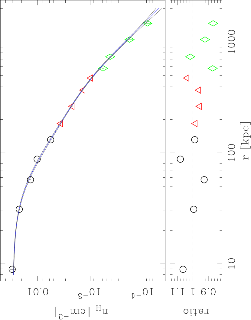
Figure 1.— Upper panel: the deprojected hydrogen density profile. The central continuous curve is the best-fit profile yielded by our analytical deprojection with the double beta-function (see Equation [6]). The other curves are the upper and lower boundaries corresponding to a one-sigma error in the parameters (see text). The markers show the data and error bars from Ettori’s matrix geometrical deprojection. Circles correspond to Chandra data, triangles to XMM-Newton and diamonds to Beppo-SAX. Lower panel : the ratio between the hydrogen density derived from the geometrical and the analytical deprojection.

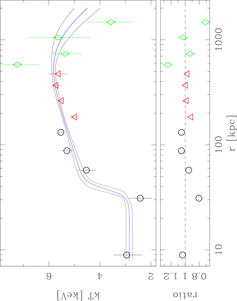
Figure 2.— Upper panel: the deprojected temperature profile, whose functional form is given by Equation (8). The meaning of the symbols is the same as in Figure 1. Lower panel : the ratio between the temperature derived from the geometrical and the analytical deprojection.

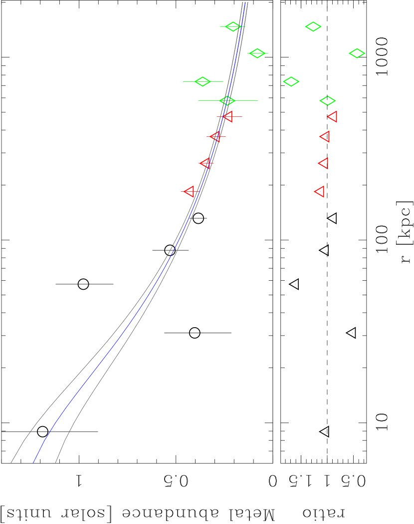
Figure 3.— Upper panel: the deprojected metal abundance profile, with functional form (9). The meaning of the symbols is the same as in Figures 1 and 2. Lower panel : the ratio between the metal abundance derived from the geometrical and the analytical deprojection.

Figure 4.— The $\Delta\chi^{2}$ on two fit parameters, obtained by running the XSPEC command steppar. Left panel: the $\Delta\chi^{2}$ on the exponent $\beta_{c}$ of the hydrogen cluster component. Despite the presence of secondary minima, the best-fit value of this parameter is robust. Right panel: the same plot for the exponent $\xi$ of the temperature profile shows a much smoother behavior.

Figure 5.— For any ring, the best-fit spectrum plotted over the data (upper panels). The lower panels show the residuals of the model, plotted as ratio data/model. Panels 1-5 refer to Chandra, 6-9 to XMM-Newton and 10-13 to Beppo-SAX.

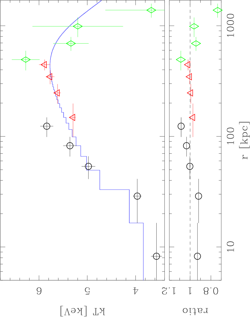
Figure 6.— Upper panel: the re-projected temperature profile plotted over the corresponding 2-D measures provided by the mekal analysis. Lower panel: the ratio between the measured emission-weighted temperature and the corresponding re-projected values.

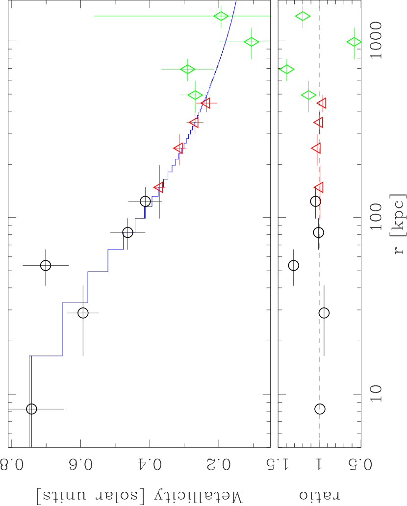
Figure 7.— Upper panel: the re-projected metallicity profile plotted over the corresponding 2-D measures. Lower panel: the ratio between the measured emission-weighted metal abundance and the corresponding re-projected values.

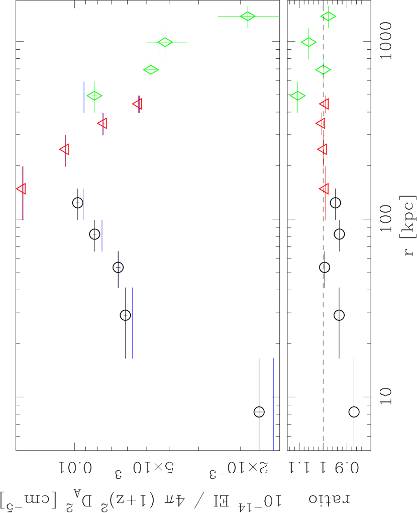
Figure 8.— Upper panel: The re-projected profile of the emission integral $EI=\int dVn_{e}n_{H}$ plotted over its corresponding 2-D measured counterpart. In the y axis $D_{A}=3.4\times 10^{2}$ Mpc and $z=0.0631$ are respectively the angular distance and the redshift of A1795. As before, circles indicates Chandra data, triangles XMM-Newton data and diamonds Beppo-SAX data. The observed quantities stem directly from the normalization of the spectra yielded by the mekal analysis. The re-projected quantities have been calculated by evaluating numerically the emission integral from the best-fit hydrogen density profile. Lower panel: The ratio between the mekal emission integral and our reprojected value.

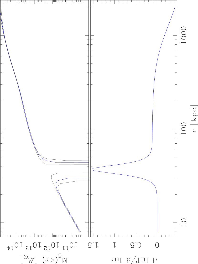
Figure 9.— The gravitating mass calculated with Equation (12) (upper panel). Because of the discontinuity edge in the temperature profile, the hypothesis of hydrostatic equilibrium breaks down at $\simeq 37$ kpc. This is best appreciated in the lower panel where we report the logarithmic derivative of the temperature profile.

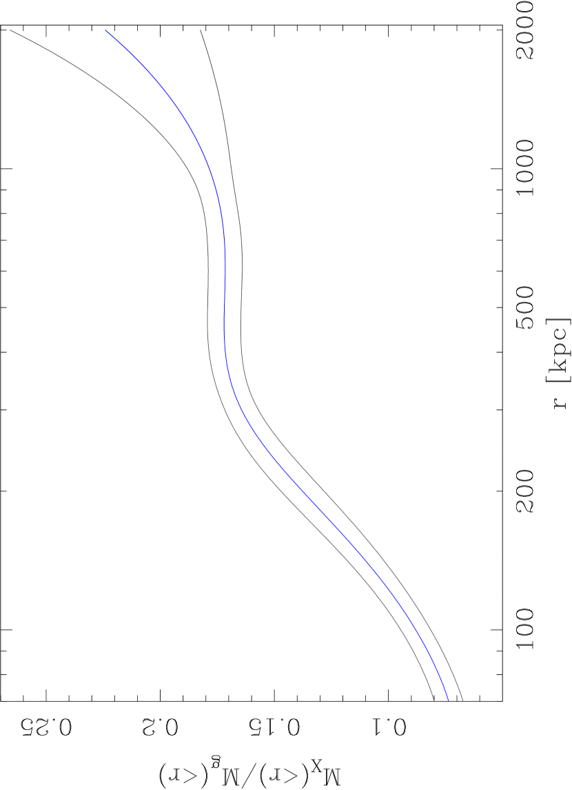
Figure 10.— The X-ray emitting gas fraction within radius $r$ is the ratio of the masses given by (13) and (12).The plot excludes the innermost region, where the hydrostatic equilibrium fails. The slight rise in the outskirts is statistically significant only at the $1$-$\sigma$ level, as discussed in Section 6.

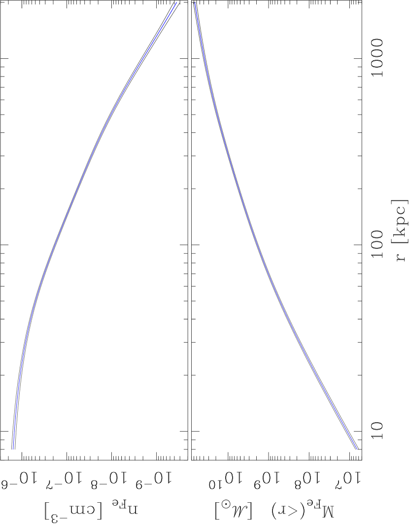
Figure 11.— The iron density (upper panel) and the enclosed iron mass within radius $r$ (lower panel). The error curves correspond to $1$-$\sigma$ uncertainty in the parameters, and have been calculated as explained in the text (Appendix C).

Table 1Extraction regions for the spectra

Instrument	Cross	Spectral range	Inner ring	Outer ring	Shading
	normalization	[keV]	[arcsec]	[arcsec]	factor
Chandra	106$\%$	0.5–7.0	0	10	1.000
		0.5–7.0	10	25	1.000
		1.0–7.0	25	40	1.000
		1.0–7.0	40	60	1.000
		1.0–7.0	60	90	1.000
XMM-Newton	100$\%$	1.0–10.0	60	120	1.000
		1.0–10.0	120	180	1.000
		1.0–10.0	180	240	1.000
		1.0–10.0	240	300	0.981
Beppo-SAX	95$\%$	2.0–10.0	240	360	1.000
		2.0–10.0	360	480	0.981
		3.5–10.0	480	720	1.000
		2.0–8.0	720	960	0.794

Note. — The cross-normalization constants among the instruments are free parameters of the model. The value relative to XMM-Newton is taken as unity by definition. The shading factor takes into account the reduced area of the extraction region of two Beppo-SAX spectra due to the entrance window.

Table 2Results for the smaug model.

Free parameter	Best-fit value	One-sigma error	Units
$f$	$4.41\times 10^{-2}$	$1.40\times 10^{-2}$	–
$n_{0}$	$2.89\times 10^{-2}$	$8.91\times 10^{-4}$	cm-3
$\beta_{c}$	$1.76$	$7.26\times 10^{-1}$	–
$r_{c}$	$5.03\times 10^{-1}$	$1.58\times 10^{-1}$	Mpc
$\beta_{g}$	$8.76\times 10^{-1}$	$5.72\times 10^{-2}$	–
$r_{g}$	$5.07\times 10^{-2}$	$2.40\times 10^{-3}$	Mpc
$Z_{0}$	$1.35$	$1.34\times 10^{-1}$	solar
$\zeta$	$2.05\times 10^{-1}$	$1.60\times 10^{-2}$	–
$T_{0}$	$2.85$	$1.27\times 10^{-1}$	keV
$T_{1}$	$6.55$	$6.20\times 10^{-1}$	keV
$r_{\rm iso}$	$3.75\times 10{-2}$	$3.37\times 10^{-3}$	Mpc
$\xi$	$3.94\times 10^{-1}$	$9.13\times 10^{-2}$	–
$r_{\rm tail}$	$1.26$	$5.80\times 10^{-1}$	Mpc

Note. — The parameters not listed are the column density of Galactic absorption $n_{H}=1.21\times 10^{-22}$ cm^-2, $\varkappa$ frozen to 10, $r_{Z}$ frozen to $8.24$ kpc i.e. one-half of the innermost radial bin, $r_{\rm cool}$ (set equal to $r_{c}$) and $\omega=0.2\,\beta_{c}$.

Table 3Checking the temperature distribution.

Profile	Free parameters	$\chi^{2}$	Degrees of freedom	F-test statistic value
isothermal	$T_{0}$	4050.8	3035	82.7
beta law	$T_{0}$ $r_{\rm tail}$ $\omega$	3731.1	3033	32.7
polytropic	$\dagger$	3781.1	3034	35.6
best-fit	$T_{0}$ $T_{1}$ $r_{\rm iso}$ $\xi$ $r_{\rm tail}$	3652.3	3031	–

Note. — The number of free parameters required to describe correctly the temperature distribution. In the beta-model the exponent is free. The F-test statistic values compare the model of each line with respect to the best-fit one. In the row of the polytropic temperature model the names of the free parameters have not been reported, since the function (8) has been modified. In this case, the temperature 3-D distribution is described by two parameters. In all cases the associated probability is well below $10^{-10}$, and has not been reported.

References

- (1) Allen, S. W., Ettori, S., & Fabian, A. C., 2001, MNRAS, 324, 877 (astro-ph/0008517 )
- (2)
- (3) Arnaud K., & Dorman B. 2000, An X-Ray Spectral Fitting Package User’s guide for version 11.0x, NASA/GSFC HEASARC Laboratory for High Energy Astrophysics
- (4)
- (5) Buote D.A., 2000, ApJ 539, 172
- (6)
- (7) David, L.P., Nulsen, P.E.J., McNamara, B.R. Forman,W., Jones,C., Ponman,T., Robertson,B., Wise, M., 2001, ApJ. 557, 546
- (8)
- (9) De Grandi, S., & Molendi, S. 2001, ApJ, 551, 153
- (10)
- (11) De Grandi, S., & Molendi, S. 2002, ApJ, 567, 1
- (12)
- (13) Ettori, S. 2000, MNRAS 318, 1041
- (14)
- (15) Ettori, S., Fabian, A. C., Allen, S. W., Johnstone, R. M. 2002, MNRAS, 331, 635
- (16)
- (17) Fabian, A. C., Hu, E. M., Cowie, L. L., Grindlay, J. 1981, ApJ 248, 47.
- (18)
- (19) Fabian, A. C., Sanders, J. S., Ettori, S., Taylor, G. B., Allen, S. W., Crawford, C. S., Iwasawa, K., Johnstone, R. M. 2001, MNRAS, 321, L33
- (20)
- (21) Johnstone, R. M., Allen, S. W., Fabian, A. C., Sanders J. S. 2002, MNRAS, in the press (astro-ph/0202071)
- (22)
- (23) Kriss, G.A., Cioffi, D.F. & Canizares, C.R. 1983, ApJ, 272, 439.
- (24)
- (25) Lang, S. 1966, Linear Algebra, (Reading, Mass.: Addison-Wesley Publishing Co.)
- (26)
- (27) Markevitch, M., Forman, W. R., Sarazin, C. L., Vikhlinin, A. 1998, ApJ, 503, 77.
- (28)
- (29) Markevitch, M., Vikhlinin, A., & Mazzotta, P. 2001, ApJ, 562, L153
- (30)
- (31) McLaughlin, D.E. 1999 , AJ, 117, 2398
- (32)
- (33) Mohr, J. J., Mathiesen B., & Evrard, A. E. 1999, ApJ, 517, 627
- (34)
- (35) Molendi, S., & Gastaldello, F. 2001, A&A, 375, L14
- (36)
- (37) Molendi, S., & Pizzolato, F. 2001, ApJ, 560, 194
- (38)
- (39) Press W.H., Teukolsky S.A., Vetterling W.T., Flannery B.P. 1992, Numerical Recipes in C (Cambridge: Cambridge University Press)
- (40)
- (41) Rybicki, G.B., & Lightman, A.P. 1979, Radiative Processes in Astrophysics, (New York: Wiley-Interscience)
- (42)
- (43) Sanders, J. S., & Fabian, A. C. 2002, MNRAS, 331, 273
- (44)
- (45) Sarazin, C.L. 1988, X-ray emission from clusters of galaxies, (Cambridge: Cambridge University Press)
- (46)
- (47) Schmidt, R. W., Allen, S. W., Fabian, A. C. 2001, MNRAS, 327, 1057
- (48)
- (49) Schmidt R. W., Fabian, A. C., & Sanders J. S. 2002, MNRAS, in the press (astro-ph/0207290)
- (50)
- (51) Tamura, T., Bleeker, J. A. M., Kaastra, J. S., Ferrigno, C., Molendi, S. 2001, A&A, 379, 107
- (52)