Entropy scaling in galaxy clusters: insights from an XMM-Newton observation of the poor cluster A1983

An XMM-Newton observation of the cool (${\rm k}T=2.1\leavevmode\nobreak\ \rm keV$) cluster A1983, at $z=0.044$, is presented. Gas density and temperature profiles are calculated over the radial range up to $500\leavevmode\nobreak\ {\rm h_{50}^{-1}\leavevmode\nobreak\ kpc}$, corresponding to $\sim 0.35\leavevmode\nobreak\ r_{200}$. The outer regions of the surface brightness profile are well described with a $\beta$-model with $\beta=0.74$, but the central regions require the introduction of a second component. The temperature profile is flat at the exterior with a slight dip towards the centre. The total mass profile, calculated from the temperature and density information assuming hydrostatic equilibrium, is consistent with an NFW profile, but with a low concentration parameter $c=3.75\pm 0.74$, which may be due to the cluster not being totally relaxed. Published optical data are used to calculate the $M/L_{\rm B}$ ratio profile and the overall iron mass over luminosity ratio. The $M/L_{\rm B}$ ratio profile shows that, at large scale, light traces mass to a reasonable extent, and the $M/L_{\rm B}$ ratio at $0.35r_{200}$ ($M/L_{\rm B}=135\pm 45\ h_{50}M_{\odot}/L{\odot}$) is consistent with the trends with mass observed in the optical. The iron mass over luminosity ratio is about two times less than that observed for a cluster at 5 keV. The gas mass fraction rises rapidly in the central regions to level off quickly at $\sim 200\leavevmode\nobreak\ {\rm h_{50}^{-1}\leavevmode\nobreak\ kpc}$; the value at $0.35\leavevmode\nobreak\ r_{200}$ is $\sim 8\%$. The scaling properties of the emission measure profile are consistent with the empirical relation $M_{\rm gas}$$\propto T^{1.94}$; use of the standard self-similar relation $M_{\rm gas}$$\propto T^{1.5}$ results in a scaled profile that is a factor of about two too low as compared to the reference mean profile for hot clusters. Comparison of the entropy profile of this cool cluster with that of the hot cluster A1413 shows that the two profiles are extremely well scaled using the empirically determined relation $S\propto T^{0.65}$, suggesting that the slope of the $S$–$T$ relation is shallower than expected in the standard self-similar model. The form of the two entropy profiles is remarkably similar, and there is no sign of a larger isentropic core in the cooler cluster. These data provide powerful agruments against preheating models. In turn, there is now increasing observational support for a trend of $f_{\rm gas}$ with system mass, which may go some way towards explaining the observed scaling behaviour.

1 Introduction

In the simplest models of gravitational collapse (e.g., Bertschinger bert85 (1985)), supported by numerical simulations without non-gravitational gas processes (e.g., Navarro, Frenk & White nfw97 (1997) [NFW]) and analytical models (e.g., Cavaliere, Menci & Tozzi cmt99 (1999)), the intrinsic properties of galaxy clusters (e.g., X-ray luminosity and temperature $L_{\rm X},T$, virial mass $M_{\rm V}$) follow self-similar scaling derived, assuming HE, from basic virial relations. Such self-similarity applies equally to the hot intracluster medium (ICM) and the dark matter components. In particular, $M_{\rm\delta}\propto T^{3/2}$, where $M_{\rm\delta}$ is the total mass in a sphere of radius $R_{\rm\delta}$ corresponding to the overall density contrast $\delta$, and $T$ is the cluster X-ray temperature. The virialised part of a cluster roughly corresponds to $\delta=200$ (e.g., Evrard, Metzler & Navarro emn96 (1996)). Assuming a constant gas mass fraction $f_{\rm gas}$= $M_{\rm gas}$$/M_{\rm V}$, the total gas mass then scales as $M_{\rm gas}$$\propto T^{3/2}$. Furthermore, if the X-ray emission is dominated by Bremsstrahlung, then $L_{\rm X}\propto T^{2}$.

However, it has been known for more than a decade that real clusters do not follow these laws (e.g., Edge & Stewart es91 (1991)). The most notable example is perhaps the $L_{\rm X}$–$T$ relation, with observations suggesting $L_{\rm X}\propto T^{\sim 2.9}$ (e.g., Arnaud & Evrard ae99 (1999)). In the study of why observed cluster properties deviate from the expected scalings, it is the $L_{\rm X}$–$T$ relation which has been in the spotlight, mainly because this relation deals with easily observable global properties. Other important scaling relations exist, however. Of particular interest for the present work are the $M_{\rm gas}$–$T$ and entropy $S$–$T$ relations, because both of these relations probe variations in gas content and can directly be derived from the data.

Studies of large samples, such as those by Neumann & Arnaud (na01 (2001)) and Mohr, Mathiesen & Evrard (mme99 (1999)) have shown that, in fact, $M_{\rm gas}$$\propto T^{1.9}$, a steepening which can be interpreted as a dependence of $f_{\rm gas}$ on temperature. However, the direct calculation of $f_{\rm gas}$ is fraught with difficulties, requiring a robust method for calculating the total mass $M_{\rm V}$, and so whether $f_{\rm gas}$ does depend on temperature is still under debate (e.g., Arnaud & Evrard ae99 (1999), Mohr et al.  mme99 (1999), Roussel, Sadat & Blanchard rsb00 (2000)).

The entropy is a formidable tool for studying the thermodynamic history of the ICM (e.g., Voit et al voitetal03 (2003)). Defining the ‘entropy’ as $S=T/n_{\rm e}^{2/3}$ (e.g., Lloyd-Davies, Ponman & Cannon ldpc00 (2000)), self-similarity implies a simple scaling of the entropy with temperature, such that $S\propto T$. Ponman, Cannon & Navarro (pcn99 (1999)) and Lloyd-Davies et al. (ldpc00 (2000)) used ROSAT observations directly to detect entropies exceeding levels attainable through gravitational collapse alone, in the inner regions (0.1 $r_{200}$) of low mass systems. From their sample of 20 systems, it appeared that the entropy followed the expected self-similar scaling down to a certain floor level of $140\leavevmode\nobreak\ {\rm h_{50}^{-1/3}}\leavevmode\nobreak\ \rm keV\leavevmode\nobreak\ {\rm cm^{2}}$, implying that non-gravitational processes act to set a lower limit to the entropy possible for the gas in collapsed haloes. However, very recent results with a much larger sample of 66 systems (Ponman, Sanderson & Finoguenov psf03 (2003)), indicate that, in fact, there exists a slope in $S(T)$ which is significantly shallower than the self-similar relation throughout, such that $S\propto T^{\sim 0.65}$. This again calls into question the fundamental assumption of a constant $f_{\rm gas}$.

The commonest explanation for the deviation from simple self-similar scaling requires non-gravitational energy input, raising the gas to a higher entropy level at some time in its history. However, there is little consensus regarding the source of this extra entropy. Pre-heating has been suggested (originally by Kaiser kaiser91 (1991) and Evrard & Henry evrard91 (1991)), although there is no agreement on the astrophysical source responsible for it: early galactic winds (e.g., Loewenstein loewenstein (2000)), AGN (Valageas & Silk valageas (1999)), or possibly both. Other effects may also play a role, like radiative cooling (e.g., Muanwong et al.  muan01 (2001)), or variation of galaxy formation efficiency with system mass (Bryan bryan00 (1998)).

Cool clusters are ideal targets for investigating the entropy because in such systems, the excess entropy becomes more evident as the processes which produce it affect the ICM in direct competition with standard gravitational heating. A1983 is well studied in optical, with $\sim 125$ galaxy velocities measured in the field by Dressler & Shectman (ds88 (1988)). Girardi et al. (getal93 (1993)) derive a velocity dispersion of $551^{+71}_{-47}$ km s^-1 from these data, a relatively low value which implies that A1983 is a cool/poor cluster.

In contrast, A1983 is little studied in X-ray. It was observed with Einstein (Jones & Forman jf84 (1984)), giving $L_{\rm X}\ [0.5-3.0]\ \rm keV=2.12\pm 0.44\times 10^{43}$ erg s^-1, and has been detected in the ROSAT All Sky Survey (Ebeling et al.  ebeling (1988)) with a quoted $L_{\rm X}\ [0.1-2.4\ \rm keV]=0.47\times 10^{44}$ erg s^-1. These low $L_{\rm X}$ values again point to the poor nature of the cluster.

This paper first presents results from the new XMM-Newton observation of A1983. The entropy and emission measure profiles of this cool cluster are then compared with those of hot clusters. These are two emphases: a direct comparison in form between the radial profiles, which shows the unparalleled quality of these XMM-Newton data; and how the scaling relations involving these quantities varies across the temperature range between the clusters. This paper will show the remarkable similarity in form between the profiles which is difficult to reconcile with conventional preheating models, and will use the $M_{\rm gas}$–$T$ and $S$–$T$ relations to argue that the gas mass fraction $f_{\rm gas}$ cannot be constant with cluster mass.

Taking $H_{0}=50$ km s^-1 Mpc^-1 and $\Omega_{0}=1$, 1′ corresponds to 71.4 kpc at the cluster redshift of 0.044.

2 Data preparation and analysis

2.1 Preliminaries

The XMM-Newton observations of A1983 were taken in Revolution 400, on 2002 February 14, and have a total exposure time of $\sim 32$ ks. Pipeline products provided by the XMM-Newton SOC, consisting of calibrated event files preprocessed with the SAS, are used in this analysis. All camera exposures used the THIN1 filter. The MOS exposures were taken in standard Full Frame mode, and for these files PATTERNs 1-12 were considered. The pn observations were obtained in Extended Full Frame (EFF) mode. In view of the calibration uncertainties associated with the EFF mode, only PATTERN 0 was considered, corresponding to the well-calibrated single events.

The dedicated blank-sky event files accumulated by Lumb (lumb (2002)) were used as background files. Events were extracted from each event file according to the same PATTERN selection as used for the source observations. The background files were then recast into the coordinates of the source observation, ensuring that source and background products are extracted from the same regions of the detector, thus minmising detector variations.

To ensure that all output products (spectra, surface brightness profiles, images) are corrected for vignetting, the photon weighting method of Arnaud et al. (arnaudetal01a (2001)) was used. This is applied to both source and background data sets. Note that while the background component induced by cosmic rays is not vignetted, source and background event files are treated in the same way, so that the correction factor is the same and thus cancels.

2.2 Flare removal

Inspection of the MOS light curves in the source-free [10-12] keV band (Fig. 1) shows that the background level during this observation is not constant. The MOS [10-12] keV light curves are very similar to the pn [12-14] keV light curve. These high energy curves show that the overall level seems to be slowly increasing, with some low-level flaring activity appearing near the end of the observation. The fluctuations are not large in these bands, but could potentially have an effect on spectra in the outer regions of the cluster, where the emission begins to be dominated by the background.

However, inspecting the light curves at lower energies, it is obvious that, for this observation at least, any criterion applied in the high energy band would miss some flares which appear to reach peak amplitude in lower energy bands.

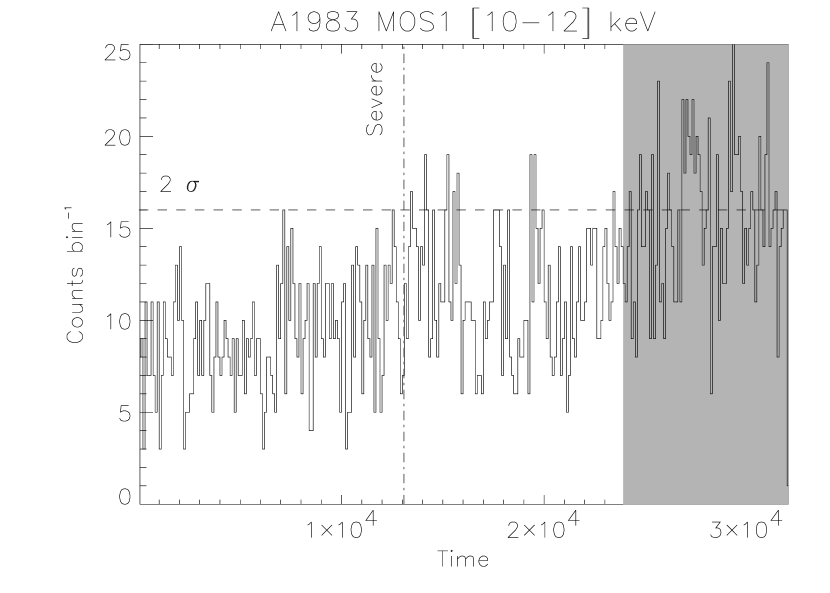
Figure 1: The MOS1 light curve in the [10-12] keV band. All frames in the shaded area were excluded because of flare activity. The 2$\sigma$ cutoff level (dotted line), established after excluding the shaded region, and the frames used for the “severe” analysis (dot-dash line), are also shown. Further details in the text.

It is prudent to exclude all frames near the end of the observation (the last $\sim 5$ ks), where flaring begins to become important. To test the effect of imposing different flare cutoff thresholds, three event files were then produced, filtered at different levels of severity, increasingly diminishing the final exposure times. The background event lists were treated using exactly the same criteria.

1. In the “$2\sigma$” event list, using the [10-12] keV light curve, frames were excluded which were outside a $2\sigma$ threshold according to the method outlined in Pratt & Arnaud (pa02 (2002)). The final exposure times are 23/16 ks (MOS/pn).

2. There are some observations where low-energy flares exist which do not appear at high energies. Light curves were thus extracted in several bands. For the MOS detectors, these bands were [0.3-1.4], [2.0-5.0], [5.0-8.0], [8.0-10.0] and [10.0-12.0] keV. For the pn, the [8.0-10.0] keV band was ignored because of strong instrumental lines, but a further light curve was extracted from events with energies between [12.0-14.0] keV. The $2\sigma$ filtering described above was then applied to each light curve, generating 5 GTI files. The observation was then filtered using the intersection of all these GTI files for a final “intersect” event list. The resulting exposure times are 18/12 ks (MOS/pn).

3. The first $\sim 13$ ks of the observation appears to be relatively quiescent, and has a mean count rate similar to that of the background files. A “severe” event list was generated by discarding all frames after this period, leaving 13/8 ks (MOS/pn) of useful data.

After masking extraneous sources, surface brightness profiles were extracted from each event list in several different bands. These profiles were background subtracted and compared. They are identical within their errors apart from differences in normalisation. To assess the effect of the filtering on spectral products, spectra were extracted in annular regions, centred on the peak of the X-ray emission from the cluster (this is is discussed in more detail below). The annular spectra from each event file were fitted with a MEKAL model at the redshift of the cluster, absorbed with the galactic absorption. MOS1, MOS2 and pn files were fitted both independently and simultaneously. The profiles from each event file were again consistent within their errors.

It thus appears that the different flare filtering levels have little or no effect on the main output products, likely due to the relatively weak nature of the fluctuations. It is nevertheless important to establish this, as incomplete flare screening has been suggested as a source of discrepancy between XMM-Newton and Chandra observations of A1835 (Markevitch mark02 (2002)). In an effort to strike a delicate balance between enthusiasm and caution, the “intersect” event lists are thus adopted for the remainder of this analysis.

2.3 Background subtraction

For each of the output products (spectra and surface brightness profiles), an equivalent product is extracted from the corresponding blank-sky event list. As discussed extensively in Pratt et al. (pa01 (2001)) and Arnaud et al. (aml02 (2002)), while the blank-sky observations provide an adequate description of the hard X-ray and instrumental components of the XMM-Newton background, they do not necessarily represent the soft X-ray component of the background, because this is variable across the sky (see Snowden et al.  snow97 (1997)). The method described in Pratt et al. (pa01 (2001)) and Arnaud et al. (aml02 (2002)) is used to correct for the difference of the background at low energy. This correction is applied to all spectra and surface brightness profiles discussed below.

The cosmic ray background is variable at the $\sim 10\%$-level, and so it is frequently necessary to normalise the background to the level of the observation. The count rate in the [10-12] keV and [12-14] keV (pn) bands, for MOS and pn respectively, is used in this analysis, with each camera treated separately.

3 Gas density distribution

3.1 Morphology

An XMM/DSS overlay image is shown in Fig. 2. The cluster exhibits morphologically symmetric X-ray emission, centred exactly on the early type galaxy [WCB96] ACO 1983 B, at $z=0.04405$ (Wegner et al.  WCB96 (1996); WCS99 (1999)). Note that this galaxy is not the Brightest Cluster Galaxy as defined by Postman & Lauer (PL (1995)), which is located $12\arcmin$ further away in the North, well beyond the X–ray emission, but the second ranked galaxy: [PL95] ACO 1983 G2.

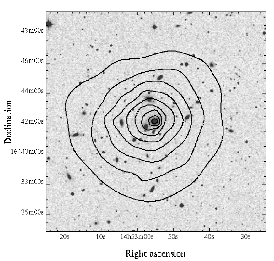
Figure 2: An XMM/DSS overlay image. The X-ray contours are from an adaptively smoothed [0.3-2.0] keV non-background subtracted MOS+pn image, and are logarithmically spaced by 0.15 dex with the lowest contour at $4.2\times 10^{-3}$ cts s^-1 arcmin².

3.2 Surface brightness profile

Tha gas density profile can be derived from the surface brightness profile, knowing the emissivity in the considered energy band. This is however more tricky for cool clusters than for hot clusters. For clusters like A1983 (${\rm k}T\sim 2\leavevmode\nobreak\ \rm keV$), the exponential cut-off of the bremsstrahlung emission lies at low energies ($E\sim{\rm k}T$). Furthermore, line emission is prominent, specially the FeL blend (see Fig. 4) and radiative recombination radiation contributes significantly to the continuum. The emissivity, $\Lambda$, in any considered energy band thus depends sensitively on the abundance and temperature. As will be seen below (see Sect. 4.3 and Sect. 4.6) radial variations of these quantities exist in the cluster centre. Thus, the corresponding $\Lambda$ profile has to be taken into account in the derivation of the gas density profile from the surface brightness. The fact that the temperature and abundance profiles are determined with a cruder spatial resolution than the $S_{\rm X}$ profile introduces a second complication and is a potential source of systematic uncertainties. The surface brightness profile was thus extracted in the [0.3-3.0] keV band with the [0.9-1.2] keV band excluded to minimise the contribution from the FeL blend, the feature which is the most sensitive to abundance and temperature.

For each camera, the azimuthally averaged surface brightness profile of the cluster and corresponding background was produced, after masking of bright sources identified in the SAS pipeline detection. The profiles were made directly from the event files by binning weighted events into circular annuli about the emission peak. The background subtraction, performed as described above in Sect 2.3, was undertaken separately for each camera. The resulting profiles are in excellent agreement with each other (bar the expected normalisation factor), and so the MOS and pn profiles were coadded. The total profile was then rebinned so that a $S/N$ ratio of $3\sigma$ was reached.

The background subtracted surface brightness profile was then corrected for the remaining radial variation of $\Lambda$. For that purpose a parametric model (in the form of Eq. 2) was used for the derived abundance and temperature profiles. The corresponding emissivity profile $\Lambda(\theta)$ was then computed in the considered energy band using an absorbed thermal model convolved with the instrumental response. The observed surface brightness profile was then divided by $\Lambda(\theta)$ normalised to its value at large radii. This correction is about $50\%$ for the central bin, but drops to about $10\%$ at $\theta\sim 0.3^{\prime}\sim 20$ kpc, and is negligable beyond $\sim 1\arcmin$.

This corrected $S_{\rm X}$ profile is shown in Fig. 3. Cluster emission is significantly detected out to $8\arcmin.4$ or $\sim 600$ kpc. It is now directly proportional to the emission measure profile, $EM(r)=\int_{r}^{\infty}n_{\rm e}^{2}\leavevmode\nobreak\ dl$, where $n_{\rm e}$ is the electronic density, which can be derived using the emissivity at large radii.

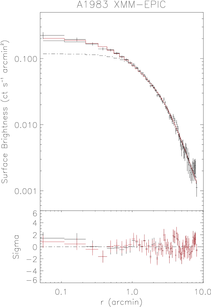
Figure 3: The combined EPIC surface brightness profile of A1983 in the [0.3-3.0] keV band, with the [0.9-1.2] keV band excluded and corrected for the dependence of the emissivity, $\Lambda$, on the temperature and abundance. The profile is background subtracted and corrected for vignetting. Dot-dash line: best fit $\beta$-model to the outer ($\theta>1\arcmin.0$) cluster region. The black and red lines are the best fit BB and KBB models convolved with the XMM-Newton PSF. See Sect. 3.3 for model details and Table 1 for the best-fit parameter values.

Table 1: Results of analytical fits to the gas surface brightness profile, errors are $90\%$ confidence.

Parameter	KBB model	BB model
$n_{\rm H,0}({\rm h_{50}^{1/2}\leavevmode\nobreak\ cm^{-3}})$	$6.64\times 10^{-3}$	$4.66\times 10^{-3}$
$r_{\rm c}$	$2\arcmin.42^{+1.03}_{-0.28}$	$2\arcmin.65^{+0.73}_{-0.56}$
$\beta$	$0.73^{+0.16}_{-0.05}$	$0.76^{+0.13}_{-0.08}$
$R_{\rm cut}$	$2\arcmin.16^{+1.19}_{-0.10}$	$2\arcmin.40^{+0.55}_{-0.54}$
$r_{\rm c,in}$	$0\arcmin.40{}_{-0.15}$	$0\arcmin.49^{+0.16}_{-0.19}$
$\xi$	$0.63^{+0.29}_{-0.34}$	-
$\chi^{2}$/d.o.f	70.36/63	70.71/64
$\chi^{2}_{\nu}$	1.12	1.10

3.3 Gas density profile

It is convenient, especially for the total mass determination below (Sect. 6), to have an analytical description of the gas density profile at all radii. The surface brightness profile $S(\theta)$ was thus fitted with various parametric models, all of which were convolved with the XMM-Newton PSF and binned in the same way as the observed profile.

A standard $\beta$-model is a good description of the outer regions, but fails nearer the centre ($\theta<1\arcmin$), where the data show a slight excess above that predicted from the fit. Progressively cutting the central region decreases the reduced $\chi^{2}$. For the single $\beta$-model, the $\chi^{2}$ becomes stable after the inner $\sim 1\arcmin$ is excised; the fit results give $\beta=0.65\pm 0.04$ and $r_{\rm c}=1\arcmin.81^{+0.21}_{-0.20}$, with $\chi^{2}=78.52/60\ {\rm d.o.f}$.

Pratt & Arnaud (pa02 (2002)) discuss alternative parameterisations for cases where a central excess is seen. These data were thus fitted with their double isothermal $\beta$-model (BB) and the generalised double $\beta$-model (KBB); the latter allowing a more centrally peaked gas density profile The resulting best fit models are given in Table 1. Note that the profile obtained beyond $R_{\rm cut}$ for the BB and KBB models is a classic $\beta$-model.

The BB and KBB models can be compared using an F-test. The F-test indicates that the KBB model is a better fit at the $42\%$ confidence level, suggesting that the density distribution in the core is not significantly more peaked than for a conventional $\beta$-model. The BB model is thus adopted for the remainder of this analysis.

4 Temperature and abundance distribution

4.1 Preliminaries

In the following, source and background spectra were extracted from the weighted event lists. In the case of the pn, these spectra were also corrected for out of time events, although in practice this makes little difference to the results. The spectra are fitted between 0.3 and 6.0 keV (cluster emission is not detected above background beyond the upper limit), and the following response matrices were used: m1_thin1v9q20t5r6_all_15.rsp (MOS1), m2_thin1v9q20t5r6_all_15.rsp (MOS2) and epn_ef20_sY9_thin.rsp (pn).

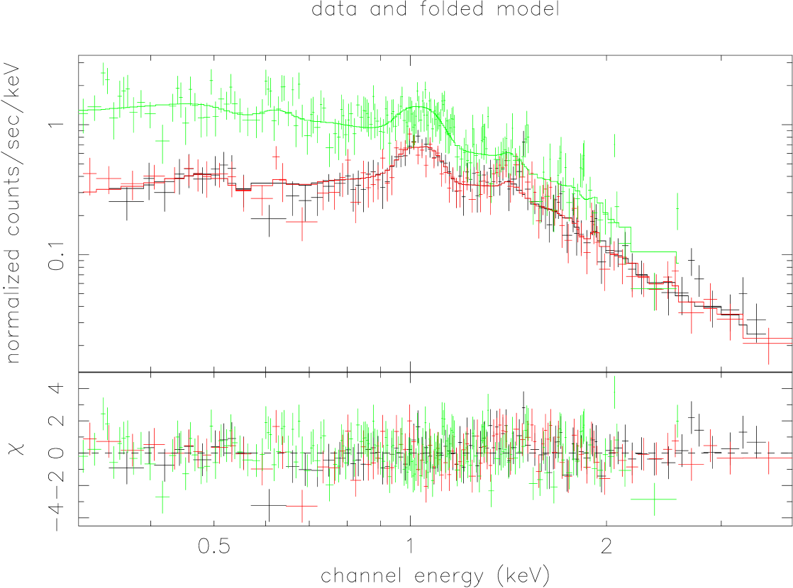
Figure 4: The global spectrum of A1983: MOS1 (black), MOS2 (red) and pn (green), shown with the best fitting combined model at $kT=2.13\pm 0.08$ keV with $Z=0.40\pm 0.05Z_{\odot}$.

4.2 Global spectrum

As a consistency check between the three cameras, a global spectrum was extracted from each event file using all events within the radius of detection (8′.4, as established in Sect. 3.3). Each spectrum was fitted with an absorbed MEKAL model with the redshift fixed at $z=0.0442$, the mean redshift of the cluster. After checking that the fit results agreed when the $N_{\rm H}$ was left free, the absorption was fixed at the galactic value of $N_{\rm H}=2.04\times 10^{20}$ cm^-2 (Dickey & Lockman dl90 (1990)); the free parameters of each fit were thus the temperature and the abundance (with respect to the solar abundances given by Anders & Grevesse agr (1989)). The global spectral fits yield $2.25^{+0.33}_{-0.12}$ keV, $2.06^{+0.13}_{-0.14}$ keV and $2.06^{+0.17}_{-0.18}$ keV for MOS1, MOS2 and pn, respectively, values which are in excellent agreement. The combined MOS/pn fit yields ${\rm k}T=2.13\pm 0.08$ keV and $Z=0.40\pm 0.05Z_{\odot}$.

The spectra are well fitted down to 0.3 keV. This is in contrast to a previous XMM-Newton observation of A1413 (Pratt & Arnaud pa02 (2002)), where, below $\sim 0.6/1.0$ keV (MOS/pn) a marked excess was seen. This could indicate that the excess in A1413 may well be a true soft excess, and not due to residual calibration problems. The global spectrum of A1983 is shown with the best fit model in Fig. 4.

4.3 Radial temperature profile

A radial temperature profile was produced by excluding point sources and extracting spectra in circular annuli centred on the peak of the X-ray emission. The widths of the rings were chosen so that a minimum $5\sigma$ detection in the [2-5] keV band was reached. This was possible for all but the final annulus. A minimum width of 30″ was also imposed, corresponding to the $90\%$ encircled energy radius of the MOS PSF. The spectra were binned to $3\sigma$ above background level to allow the use of Gaussian statistics.

The spectra were fitted with the absorbed MEKAL model described in the previous Section. In all cases the MOS normalisations were tied together, but the pn normalisation was allowed to vary. In the final two annuli, the abundance was frozen at the abundance found for the third-last annulus. Spectra from different cameras were fitted individually at first: these results are identical within their errors, and so a further simultaneous MOS+pn fit was undertaken. The results are detailed in Table 2 and shown in Fig. 5.

Table 2: Projected radial temperature profile results. Errors are $1\sigma$, as shown in Fig. 5.

Annulus	kT	$Z$
( ′ )	(keV)	($Z_{\odot}$
0.00-0.66	$1.88^{+0.07}_{-0.12}$	$0.56^{+0.07}_{-0.06}$
0.66-1.32	$1.99^{+0.08}_{-0.08}$	$0.34^{+0.05}_{-0.04}$
1.32-1.98	$2.13^{+0.08}_{-0.08}$	$0.37^{+0.06}_{-0.05}$
1.98-2.64	$2.02^{+0.10}_{-0.10}$	$0.29^{+0.06}_{-0.05}$
2.64-3.30	$2.39^{+0.22}_{-0.15}$	$0.29^{+0.09}_{-0.07}$
3.30-3.96	$2.21^{+0.25}_{-0.19}$	$0.29^{+0.10}_{-0.08}$
3.96-4.62	$2.49^{+0.35}_{-0.31}$	$0.24^{+0.12}_{-0.09}$
4.62-6.16	$2.11^{+0.19}_{-0.19}$	0.3 frozen
6.16-7.94	$2.55^{+0.91}_{-0.47}$	0.3 frozen

Figure 5: The total XMM-EPIC radial temperature profile of A1983. The solid line is the best fit to the temperature profile with a function of the form given in Eqn. 2. Errors are $1\sigma$ confidence level.

4.4 Is there a cooling flow?

The slight and gradual decrease in temperature towards the centre indicates that there might be a cooling flow (CF). Indeed this has already been suggested, on the basis of a deprojection analysis of the Einstein data by White, Jones & Forman (wjf97 (1997)), who find evidence for a weak CF of $\sim 6M_{\odot}$ yr^-1. The cooling time can be calculated using

$$t_{\rm cool}=2.9\times 10^{10}\ {\rm yr}\ \sqrt{\frac{{\rm k}T}{1\leavevmode\nobreak\ \rm keV}}\left(\frac{n_{\rm H}}{10^{-3}{\rm cm}^{-3}}\right)^{-1},$$ (1)

from Sarazin cs86 (1986). With the central density derived from the BB model fit, $t_{\rm cool}\sim 8.5\times 10^{9}$ yr. This value suggests that cooling, if indeed present, should be rather weak.

Starting from the central annulus and working outward, the spectra were fitted with an absorbed two temperature MEKAL model. Except for the central [0′- 0′.66] spectrum, the addition of a second spectral component either does not provide a significant (as defined by application of the F-test) reduction in the $\chi^{2}$, or, more often, the second component parameters are completely unconstrained.

The [0′- 0′.66] spectrum was then fitted with various models as detailed in Table 3. The best-fitting model is (very marginally) the absorbed MEKAL+MKCFLOW. The same spectrum fitted with a single temperature plus cooling flow model with $\dot{M}$ fixed to $6M_{\odot}$ yr^-1 (as obtained by White et al. wjf97 (1997)) yields $\chi^{2}_{\nu}=1.93$ and shows significant residuals below 1 keV.

Table 3: Comparison of spectral fits to the [0′- 0′.66] spectrum. The $N_{\rm H}$ has been fixed to the galactic values as detailed in Sect 4.2. All errors are given at the $90\%$ confidence level.

Model	kT	$Z$	$kT_{\rm low}$	$\dot{M}$
	(keV)	($Z_{\odot}$)	(keV)	($M_{\odot}$ yr-1)	$\chi^{2}$/d.of
wabs(mekal)	$1.88^{+0.12}_{-0.14}$	$0.56^{+0.12}_{-0.13}$	-	-	331.4/307
wabs(mekal+mekal)	$2.18^{+0.19}_{-0.16}$	$0.82^{+0.18}_{-0.08}$	$0.82^{+0.25}_{-0.17}$	-	330.4/305
wabs(mekal+mkcflow)	$2.32^{+0.32}_{-0.10}$	$0.85^{+0.18}_{-0.10}$	-	$3.20^{+0.80}_{-0.79}$	330.1/305

4.5 Projection and PSF effects

PSF and projection effects will be a particular problem if radial bins smaller than the $90\%$ encircled energy radius of the PSF are used, or if the surface brightness of the cluster is very peaked (i.e., the luminosity is concentrated towards the centre), or if there are significant temperature gradients. None of which is true for A1983: the radial temperature profile, extracted in bins with width greater than the $90\%$ encircled energy radius of the PSF, is relatively flat out to the limit of detection, and, while the surface brightness profile does show a slight peak towards the centre, this is not a large effect. In this context A1983 can be compared directly with A1413, a cluster with a relatively flat temperature profile and a peaked surface brightness distribution. The fully PSF-corrected and deprojected temperature profiles of A1413 are consistent with the projected profile within the $1\sigma$ errors. Since deprojection and/or PSF correction are likely to have little effect on the temperature profile, except to decrease the $S/N$, the projected profile is used throughout this analysis.

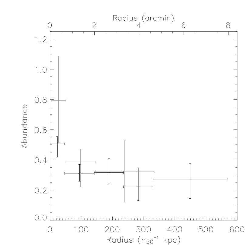
Figure 6: The radial abundance profiles for Fe (black) and Si (grey).

4.6 Abundance gradients

There is strong line emission from several elements at the average temperature of A1983, however, significant radial constraints could only be put on Fe and Si abundances. (The Mg K line falls in the energy band affected by the Al K and Si K flourescent energy lines in the MOS background, and so was ignored in the present analysis.)

The radial abundance profile of Fe shown in Fig. 6 was obtained from an absorbed VMEKAL model fit with all $\alpha$-processed elements and Fe treated as free parameters. To augment the statistics outside the centre, the spectra were reaccumulated in annuli twice the width as those used for the temperature determination. The Fe gradient is relatively flat except for the central annulus, where there is a pronounced jump from $0.3Z_{Fe,\odot}$ to $0.5Z_{Fe,\odot}$.

The spectra had to be reaccumulated in bins twice as large again for constraints to be found on the Si profile, shown in the same Figure. The Si abundance jumps from $0.4Z_{Si,\odot}$ to $0.8Z_{Si,\odot}$ in the central annulus, but outside this region the Si abundance is essentially constant. Because of the large errors on the Si abundance, it is difficult to obtain useful constraints on the radial variation of the Si/Fe abundance ratio.

4.7 Hardness ratio image

A hardness ratio (HR) image offers a relatively simple way of analysing the two-dimensional temperature structure of the cluster, and to this end, source and background images were produced in the [0.3-0.9] keV and [2.5-6.5] keV bands, chosen to avoid strong line emission. Exposure maps were generated for each image in each band using the SAS task eexpmap.

To avoid large numbers of negative pixels, especially in the external regions, it is preferable to smooth images before undertaking any mathematical operations. The SAS task asmooth allows a smoothing template to be defined, ensuring that each region of each image can be smoothed in exactly the same fashion. Since the high energy images have a lower sigal to noise ratio, the template is best defined using these images. For the present analysis, a template was defined by adaptively smoothing the MOS1 [2.5-6.5] keV image, and this template was then applied to each source and background image.

The corresponding background was normalised based on the effective exposure times and subtracted from each image. The background subtracted images were then divided by their respective exposure maps, and the hardness ratio image was calculated for each camera using HR = (image[2.5-6.5 keV]-image[0.3-1.4 keV])/(image[2.5-6.5 keV]+image[0.3-1.4 keV]). The MOS and pn results are in excellent agreement, and the combined MOS/pn HR image is shown in Fig 7.

In deriving these results, the difference between the blank-sky background and the A1983 background at low energy has been neglected. This would only affect the low-energy images as there is essentially no difference above $\sim 2$ keV, and would preferentially affect the outer regions where the background becomes a significant fraction of the detected flux. In not taking this into account, the absolute HR values will be incorrect. However, the overall temperature structure will still be well described. Tests with the annular spectra (discussed above) show that the difference between the backgrounds begins to play a role at a radius of about 6′, making the uncorrected spectra seem hotter than they actually are by about $10\%$. This would explain why the external regions of the map seem slightly harder. A direct translation of HR values into temperatures has not been attempted because of the complexity properly of treating this problem.

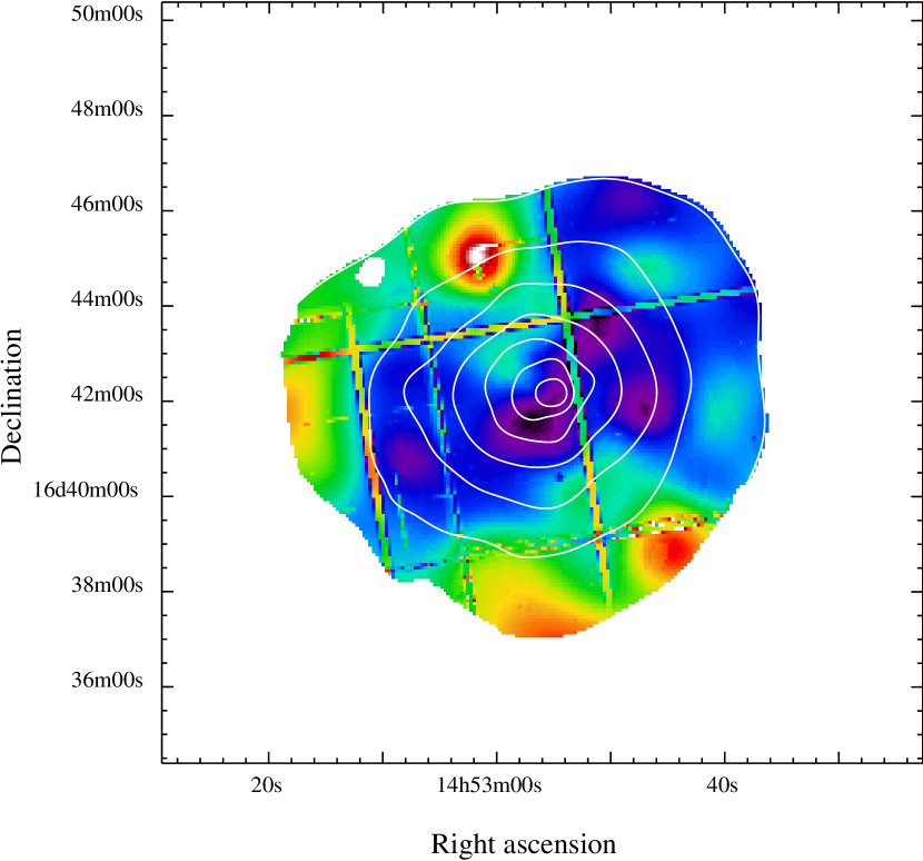
Figure 7: The hardness ratio map of the cluster extending to a radius $\sim 7\arcmin$ from the centre, from all EPIC cameras. The dynamic scale has been chosen to emphasise structure, is linear, and ranges from -0.75 (black) to -0.375 (white). The lines are due to the gaps between CCD chips.

The HR image shows quite a lot of structure, with point sources to the NE and SW of the centre standing out clearly. There appears to be a cool elongation running approximately SE-NW, which has a radial extension of $\sim 2\arcmin$ (roughly 140 kpc). However, it should be stressed that the colour table has been adjusted to emphasise any structure, and in fact, the hardness ratio variations are not large at all within the region covered by the map (as can be seen from the colourbar). As a rough guide, the variations in hardness ratio present in this image represent temperature variations of order $20\%$, a value which is entirely consistent with the radial values seen in Sect. 4.3.

Figure 8: The gas entropy ($S={\rm k}T/n_{\rm e}^{2/3}$) profile derived from the temperature profile and the double $\beta$-model (BB) for the gas density. The dotted line represents the entropy profile obtained using analytic models for the gas density and temperature distributions. The dot-dash line is the entropy obtained in the central bin if the spectrum is modelled with a two phase gas and the hotter of the two components is used to calculate the entropy.

5 Entropy profile

The gas entropy was determined from the BB analytical model fit to the gas density profile and the observed temperature profile, with entropy $S={\rm k}T/n_{\rm e}^{2/3}$. The temperature profile was also modelled with a function of the form:

$$T=T_{0}+T_{1}[(r/r_{\rm c})^{\eta}/(1+(r/r_{\rm c})^{\eta})]$$ (2)

(c.f., Allen et al.  asf01 (2001)) with $T_{0}=1.86$ keV, $T_{1}=0.41$ keV, $r_{c}=1\arcmin.46$ and $\eta=1.75$, and the entropy calculated using this profile. The resulting entropy profiles are shown in Fig. 8. The uncertainty in the entropy profile is dominated by the uncertainty on the temperature distribution. Typical errors, corresponding to the error in each bin of the temperature profile are indicated in the figure. As discussed above in Sect. 4.4, there is some evidence that the central bin may have more than one temperature component. The entropy in this central bin calculated with the hotter of the two temperature components is also shown in the Figure, it agrees with the single temperature values within their errors.

6 Mass analysis

Figure 9: Integrated total gravitating mass and gas mass distributions. The total mass is shown with $1\sigma$ errors. The dashed line shows the mass profile calculated from the analytical temperature and gas density distributions. The solid line through the points is the best fit NFW profile, with $c=3.75$ and $r_{200}=1480$. In this and subsequent Figures in Section 6, this best-fitting NFW mass model is used to compute the scaled radius given on the top axis.

6.1 Total mass profile

6.1.1 Calculation of the profile

The total gravitating mass distribution shown in Fig. 9 was calculated under the usual assumptions of hydrostatic equilibrium and spherical symmetry using

$$M(r)=-\frac{kT\ r}{{\rm G}\mu m_{p}}\left[\frac{d\ln{n_{\rm g}}}{d\ln{r}}+\frac{d\ln{T}}{d\ln{r}}\right],$$ (3)

where G and $m_{p}$ are the gravitational constant and proton mass and $\mu=0.609$. The profile itself was calculated with an adapted version of the Monte Carlo method of Neumann & Böhringer (nb95 (1995)), which takes as input the analytical parameters for the gas density profile and the measured temperature profile. The original method calculates random temperature distributions within the error bounds of the observed temperature profile, using a ‘diffusive’ process characterised by two parameters, a window size and a step parameter. A significant advantage of the method is that it guarantees a certain smoothness of the temperature profiles and thus naturally limits ‘unphysical’ profiles with large oscillations. However, for this cluster, probably due to the fluctuations observed in the temperature profile (see also below), it was found difficult to choose objectively the window and step parameters, on which depends the final dispersion on the derived mass profiles and thus the error on the mass profile. To avoid this problem, a simpler, although less efficient, way to generate random temperature profiles was used. A random temperature at each radius of the measured temperature profile was simply generated assuming a Gaussian distribution with sigma equal to the $1\sigma$ error, and a cublic spline interpolation was used to compute the derivative. As in Neumann & Böhringer (nb95 (1995)) only ‘physical’ temperature profiles are kept, i.e. those yielding to monotically increasing total mass profiles. In total 1000 such profiles were calculated.

To include the error due to the uncertainty on the modelling of the gas density profile, the error on the density gradient (i.e., ${\rm d}\ln{n_{\rm g}}/{\rm d}\ln{r}$) was calculated. For this, the surface brightness profile was fitted at each radial point with ${\rm d}\ln{n_{\rm g}}/{\rm d}\ln{r}$ as the free parameter, enabling the errors on this quantity to be calculated from the $\chi^{2}$ variation, the other parameters (normalisation, $r_{c,{\rm in}}$, $r_{c}$) having been optimised. The final uncertainty values for the mass points are derived from the quadratic addition of these errors with those due to the temperature profile (output from the Monte Carlo method). The Monte Carlo mass profile, with appropriate uncertainities, is shown in Fig. 9.

The mass profile can also be derived analytically using the temperature profile model as given in Eqn. 2 and the best fit BB model. This result, shown as the dashed line in Fig. 9, is in excellent agreement with the results from the Monte Carlo analysis.

6.1.2 Modelling of the mass profile

The total mass profile was fitted with the Navarro, Frenk & White (nfw97 (1997)) profile, given by:

$$\rho(r)=\frac{\rho_{\rm c}(z)\delta_{c}}{(r/r_{\rm s})(1+r/r_{\rm s})^{2}}$$ (4)

where $\rho(r)$ is the mass density and $\rho_{\rm c}(z)$ is the critical density at the observed redshift, which, for a matter dominated $\Omega=1,\Lambda=0$ Universe is:

$$\rho_{\rm c}(z)={\rm\frac{3H_{0}^{2}}{8\pi G}}(1+z)^{3};$$ (5)

and where $\delta_{c}$ can be expressed in terms of the equivalent concentration parameter, $c$:

$$\delta_{\rm c}=\frac{200}{3}\frac{c^{3}}{[\ln(1+c)-c/(1+c)]}.$$ (6)

The radius corresponding to a density contrast of 200 is $r_{200}=cr_{\rm s}$.

This produced a fit with $\chi^{2}=9.14/7$ d.o.f, which is not a bad fit. The best fit NFW parameters are: $c=3.75\pm 0.74$, $r_{\rm s}=394\pm 124$ kpc, giving $r_{200}=1480$ kpc and $M_{200}=2.15\times 10^{14}$ M_⊙. This best-fit NFW model is shown overplotted on the mass profile of the cluster in Fig. 9. Note that in this and other Figures in this Section, the virial radius ($r_{200}$) shown is that calculated from the NFW fit.

Figure 10: The integrated gas mass fraction as a function of radius. Errors are calculated from the quadratic combination of $1\sigma$ errors on the total mass and the gas mass. The solid line is the gas mass fraction derived from the gas mass and the best fitting NFW mass profile.

The alternative Moore et al. (mqgsl99 (1999)) profile was also tried, which is given by:

$$\rho(r)=\frac{\rho_{\rm c}(z)\delta_{c}}{(r/r_{s})^{3/2}\left[1+\left(r/r_{s}\right)^{3/2}\right]},$$ (7)

where

$$\delta_{c}=\frac{100c^{3}}{\ln{(1+c^{3/2})}}.$$ (8)

With all parameters free, this profile gives a worse fit than the NFW ($\chi^{2}=12.22/7$ d.o.f), and moreover the best-fit scale radius in this case is a rather unlikely 55 Mpc. The fit was repeated with a upper limit to the scale radius fixed at twice the best-fit NFW value (i.e., 788 kpc). Here the fit is worse again ($\chi^{2}=17.09/7$ d.o.f), but gives similar $r_{200}$ and $M_{200}$ values to the NFW fit. The best-fit scale radius value is at the maximum allowed by the fit. In the light of these results, it seems likely that these data do not have the required radial reach to put useful constraints on this model.

6.2 Gas mass profile and gas mass fraction

Figure 9 also shows the radial gas mass distribution derived from integration of the best-fit BB model. The variation in the gas mass fraction with radius is shown in Fig. 10. This figure shows that the gass mass fraction rises rather abruptly in the first 200 kpc, beyond which it stabilises at a value of $\sim 7\%$.

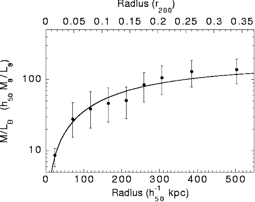
Figure 11: The integrated radial mass-to-light ratio. Errors are derived quadratically from the mass and luminosity errors in each bin. The solid line is the mass-to-light ratio determined from the best-fitting NFW mass model.

6.3 Mass to light ratio

The extensive optical observations of A1983 can be used to derive the radial mass-to-light ratio, which is an indication of the extent to which the light traces the mass.

The contribution of the Central galaxy (cG) was the first to be estimated. The photometric data of Saglia et al. (saglia (1997)) was used: a blue magnitude of $B=16.0$ measured in an aperture of $\theta_{\rm ap}=14.95\arcsec$, together with a surface brightness profile following a de Vaucouleurs law with an effective radius of $\theta_{\rm e}=14\arcsec$. A total B magnitude of $B=15.3$ was derived, which corresponds to a total blue luminosity of $L_{\rm B,cG}=8.8\times 10^{10}\leavevmode\nobreak\ \rm h_{50}^{-2}\leavevmode\nobreak\ L_{\odot}$ for a galactic extinction of $A_{\rm B}=0.112$ (Schlegel et al.  schlegel (1998)). The luminosity within any radius of interest was estimated using the aproximation of Mellier & Mathez (mellier (1987)) for deprojecting the de Vaucouleur surface brightness profile.

Girardi et al. (getal02 (2002)) derive a total $B_{\rm j}$ luminosity of A1983 from APS data. After correcting for the completeness limit they obtain $L_{\rm B_{\rm j}}=5.97/7.44\times 10^{11}\leavevmode\nobreak\ {\rm L_{\odot}}$ within $0.99$ Mpc for a Hubble constant of 100 km $s^{-1}$ Mpc^-1. The two luminosity values are derived using different procedures for the fore/background correction, so the average of the two values was used. The luminosity was then converted to the B band assuming $L_{\rm B_{\rm j}}/{\rm L_{B_{j},\odot}}=1.1\leavevmode\nobreak\ L_{\rm B}/{\rm L_{B,\odot}}$ (Girardi et al.  getal02 (2002)), and the luminosity of the cG subtracted. The resulting luminosity (excluding the cG) is then $L_{\rm B}=(2.4\pm 0.2)\times 10^{12}\leavevmode\nobreak\ \rm h_{50}^{-2}\leavevmode\nobreak\ L_{\odot}$ within a projected radius of $1.98\leavevmode\nobreak\ {\rm h_{50}^{-1}}$ Mpc. A modified King profile with core radius of $r_{\rm c}=20\leavevmode\nobreak\ {\rm h_{50}^{-1}}$ kpc and $\alpha$ = 0.61 (Girardi et al.  getal95 (1995)) can then be used to model the galaxy distribution and thus interpolate the luminosity to the radius of interest. The $68\%$ errors on the profile parameters are large: $r_{\rm c}<100\leavevmode\nobreak\ {\rm h_{50}^{-1}}$ kpc and $0.5<\alpha<0.77$ (M. Girardi, private communication), and are the main sources of uncertainty. This luminosity profile was then added to the cG luminosity profile to derive the total cluster luminosity profile.

The final total mass-to-light ratio is shown in Fig. 11, where the errors are computed quadratically from the mass and luminosity errors in each bin.

6.4 Iron mass over luminosity ratio

The Iron Mass over Luminosity ratio (IMLR = $M_{\rm Fe}/L_{\rm B}$) is a fundamental quantity for the understanding of ICM enrichment (e.g. Renzini renzini (1997)). Using the Fe abundance measured at large scale ($[Fe/H]\sim 0.3$ with typically $15\%$ error) the IMLR within $0.3\leavevmode\nobreak\ r_{200}$ is IMLR $=(5.3\pm 2.2)\times 10^{-3}\leavevmode\nobreak\ \rm h_{50}^{-1/2}\leavevmode\nobreak\ M_{\odot}/L_{\odot}$. An overall IMLR was also derived by extrapolating the gas mass to $r_{200}$ and assuming that the abundance remains constant. In this case, a great deal of extrapolation is needed, and caution is advised in the interpretation of the results. On the other hand, the luminosity estimate within that radius is more robust, being less sensitive to the assumed light distribution. The overall IMLR obtained using this method is IMLR $=(8.9\pm 1.8)\times 10^{-3}\leavevmode\nobreak\ \rm h_{50}^{-1/2}\leavevmode\nobreak\ M_{\odot}/L_{\odot}$.

7 Discussion

7.1 Mass profile: comparison with theoretical expectations

There is now converging evidence that the mass profile of relatively hot clusters follows the cusped distribution predicted from numerical simulations of dark matter collapse (David et al.  david01 (2001); Arabadjis, Bautz & Garmire abg02 (2002); Allen et al.  asf01 (2001), Pratt & Arnaud pa02 (2002)). Our results suggest that this is also true for cool clusters.

The NFW profile is a relatively good fit to the A1983 data, but not as good as for instance for A1413 (Pratt & Arnaud pa02 (2002)). However, there are a several points of note. For the calculation of the mass profile, the radial temperature and gas density distributions have been used. The first and most obvious point is that the temperature distribution is not smooth. The radial temperature data used for this mass analysis exhibit fluctuations on the order of $\sim 20\%$, and this will inevitably have an effect on the quality of the NFW fit to a mass model derived using these data. Secondly, there is a point of inflection in the mass profile around $170\leavevmode\nobreak\ {\rm h_{50}^{-1}\leavevmode\nobreak\ kpc}$, corresponding to the boundary between the two $\beta$ models used to fit the surface brightness profile. In the future, our intention is to develop more robust models for the surface brightness modelling, but that is beyond the scope of this paper.

The theory of cluster formation predicts that the concentration parameter should be higher for lower mass systems (e.g. NFW). The concentration parameter of A1983, $c=3.75\pm 0.74$, is lower than would be expected for a cluster of this mass, $c\sim 9$ (e.g Eke, Navarro & Frenk enf (1998)). It is also significantly lower than the value $c=5.4\pm 0.2$ derived for A1413, a cluster about 5 times more massive (Pratt & Arnaud pa02 (2002)). However, studies of large numbers of simulated haloes by Bullock et al. (bull01 (2001)) and Thomas et al. (pat01 (2001)) has shown that there is a wide dispersion in the value of $c$, so the result is perhaps not surprising. In addition, the original NFW profile was derived from the mass distributions of equilibrium haloes; in fact NFW specifically considered earlier epochs for some of their simulated haloes, assuring equilibrium by excluding the most recently accreted subunit. As shown by Jing (jing00 (2000)), in a study of the diversity of density profiles of a large number of massive haloes, the quality of the NFW fit depends on whether the halo is in equilibrium. In particular, unrelaxed clusters yield concentration parameters lower than the NFW values. Observationally, a close look at the X-ray image of A1983 (Fig. 2) indicates that, while the isophotes are regular at large scale, there is an extension towards the NE in the central regions. Moreover, as the X-ray temperature analysis has shown (Sect. 4.7), there are radial and non-radial temperature variations of $\sim 20\%$. Lastly, previous optical observations (Escalera et al.  escetal94 (1994); Girardi et al.  getal97 (1997)) have found evidence for several substructures in the field of this cluster, at least one of which appears to cover the central region. These observational points seem to suggest that A1983 is not as relaxed as initially it may appear, presumably due to an earlier merging event which may still be detectable in the X-ray temperature and galaxy distributions. This shows the importance of knowing in detail the dynamical state of a cluster for the interpretation of the mass profile.

Large simulations, like the Hubble Volume simulation, indicate a tight correlation between $M_{200}$ and the dark matter velocity dispersion in the form of $\sigma=1075\leavevmode\nobreak\ [(E(z)\leavevmode\nobreak\ M_{200}/(10^{15}\leavevmode\nobreak\ {\rm h_{100}^{-1}\leavevmode\nobreak\ M_{\odot}})]^{1/3}$ km s^-1 (Evrard & Gioia eg (2002)), where $E(z)=H(z)/H_{0}$. The best fit NFW mass model, $M_{200}=2.15\times 10^{14}\leavevmode\nobreak\ {\rm h_{50}^{-1}\leavevmode\nobreak\ M_{\odot}}$, gives $\sigma\sim 520$ km s^-1. This is consistent with the robust, optically-derived value of the galaxy velocity dispersion $\sigma=551^{+71}_{-47}$ km s^-1. This excellent agreement indicates: i) that the total mass estimate is probably not too much in error and that the cluster cannot be too far from equilibrium, and ii) gives further support to the current modelling of the dark matter collapse.

Finally, the normalisation of the $M_{200}$–$T$ relation for this cluster, defined as $M_{10}(200)=E(z)\leavevmode\nobreak\ M_{200}\leavevmode\nobreak\ T_{10}^{-3/2}$, where $T_{10}$ is the temperature in units of 10 keV, is $M_{10}(200)\sim 2.3\times 10^{15}\leavevmode\nobreak\ {\rm h_{50}^{-1}\leavevmode\nobreak\ M_{\odot}}$. This is about $25\%$ lower than the normalisation of Evrard et al. (emn96 (1996)). We thus confirm, at a lower mass, the offset between the observed and theoretical normalisation of the $M$–$T$ relation, already observed for hot clusters (Allen et al.  asf01 (2001); Pratt & Arnaud pa02 (2002)).

7.2 Mass versus light as a function of scale

At large radii, the light seems reasonably to trace the mass. Within the relatively large errors, the mass-to-light ratio flattens beyond $\sim 0.2\leavevmode\nobreak\ r_{200}$, reaching a value of $M/L_{\rm B}=(135\pm 45)\leavevmode\nobreak\ \rm h_{50}\leavevmode\nobreak\ M_{\odot}/L_{\odot}$ at $0.3\leavevmode\nobreak\ r_{200}$ (Fig. 11). The value extrapolated at $r_{200}$, using the best fit NFW mass profile, is similar: $M/L_{\rm B}=150\leavevmode\nobreak\ \rm h_{50}\leavevmode\nobreak\ M_{\odot}/L_{\odot}$, for a luminosity within that radius of $L_{\rm B}\sim 1.4\times 10^{12}\leavevmode\nobreak\ \rm h_{50}^{-2}\leavevmode\nobreak\ L_{\odot}$ (estimated as described in Sect. 6.3).

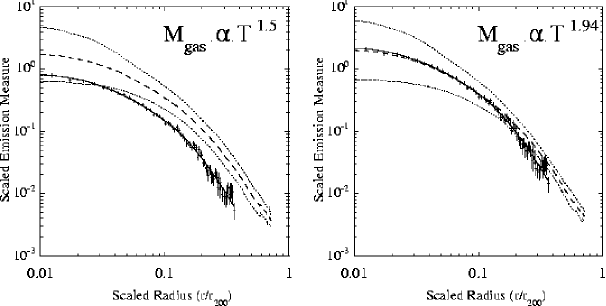
Figure 12: The scaled emission measure (EM) profile of A1983 (data points) compared to the mean scaled EM profile of the ensemble of hot clusters (${\rm k}T>3.5$ keV) observed by ROSAT and considered by Neumann & Arnaud (na01 (2001)). The latter is indicated by the dashed line; dotted lines show the dispersion. On the left, the EM profile of A1983 is scaled using the self-similar $M_{\rm gas}$$\propto T^{1.5}$ scaling. On the right, it is scaled using the empirical $M_{\rm gas}$$\propto T^{1.94}$ scaling of Neumann & Arnaud (na01 (2001))

This mass-to-light ratio value for a cluster of such a low luminosity is consistent with the general trend observed by Girardi et al. (getal02 (2002)) from poor groups to rich systems. Using a very large sample, these authors found a significant increase of $M/L$ with luminosity with a best fit power law of $M/{\rm M_{\odot}}=10^{-1.596}\leavevmode\nobreak\ (L_{\rm B}/{\rm L_{\odot}})^{1.338}$ for ${\rm H_{0}}=100$ km s^-1 Mpc^-1. Rescaling their results for ${\rm h_{50}}=1$, and using the luminosity estimated at $r_{200}$, leads to a mass-to-light ratio of $M/L_{\rm B}\sim(100\pm 20)\leavevmode\nobreak\ \rm h_{50}\leavevmode\nobreak\ M_{\odot}/L_{\odot}$, taking into account the typical dispersion around the correlation. This is within the error bars of the observed value, although somewhat on the low side.

On the other hand, David, Jones & Forman (david (1995)), who used X-ray mass estimates for a much smaller sample of 7 groups and clusters, did not find any evidence of mass-to light variation with mass. All objects in their sample fall in the range $M/L_{\rm V}=100-150\leavevmode\nobreak\ \rm h_{50}\leavevmode\nobreak\ M_{\odot}/L_{\odot}$. Similar values were derived by Cirimele, Nesci & Trevese (cirimele (1997)) from a sample of 12 clusters in the temperature range from 2 to 10 keV. Assuming $(L_{\rm V}/L_{\rm V,\odot})=1.3\leavevmode\nobreak\ (L_{\rm B}/L_{\rm B,\odot})$, relevant for early type galaxies, this translates into a mass-to-light ratio in the B band of $M/L_{\rm B}=130-200\leavevmode\nobreak\ \rm h_{50}\leavevmode\nobreak\ M_{\odot}/L_{\odot}$. It must be noted that the mass-to-light ratio of A1983 is also consistent with the David et al. (david (1995)) finding. Clearly larger homogeneous X-ray samples, of size similar to those now available in optical, are needed to see if there is a real contradiction between $M/L$ trends derived respectively from X-ray and optical mass determination methods.

The mass-to-light ratio decreases towards the central part of the cluster, where the light is dominated by the central galaxy (Fig. 11). The mass-to-light ratio in the central bin, located at 23 kpc or about 1.4 times the effective radius of the central galaxy (Sect. 6.3), is $M/L_{\rm B}=9\pm 2$. This value is consistent with the typical mass-to-light ratio of the stellar population (e.g. Gerhard et al.  gerhard (2001) and references therein). This suggests that there is little if any dark matter component in the central part of the galaxy. At $r\sim 2.8r_{e}$ the $M/L_{\rm B}$ ratio has increased to a value of $\sim 30$. Interestingly, similar values and trends have been observed both around M87, the central very bright galaxy in the Virgo cluster (Matsushita et al.  mat02 (2002)) and in isolated elliptical galaxies (Gerhard et al.  gerhard (2001)), two very different environments.

7.3 Scaling law tests

7.3.1 Testing the $M_{\rm gas}$$-T$ relation

The surface brightness profile of A1983 can be used to test the $M_{\rm gas}$$-T$ relation. The surface brightness profile of the cluster was converted into an emission measure ($EM$) profile using

$$EM(r)=\frac{4\pi(1+z)^{4}S(\theta)}{\Lambda(T,z)};\ \ r=d_{\rm A}(z),\theta$$ (9)

where $\Lambda(T,z)$ is the emissivity, taking into account the interstellar absorption and the spectral response, and $r=d_{A}(z)$ is the angular distance at redshift $z$.

This EM profile was then scaled according to the self-similar model, using the standard scaling relations of cluster properties with redshift and temperature. In the first instance, the profile was scaled using the standard relation $M_{\rm gas}$$\propto T^{1.5}$. In the left-hand panel of Fig. 12, this scaled EM profile is compared to the mean scaled EM profile of the ensemble of hot (${\rm k}T>3.5$ keV), nearby ($z<0.06$) clusters observed by ROSAT and considered by Neumann & Arnaud (na01 (2001)). It can clearly be seen that the form of the profile is similar to that observed for hotter clusters. This is interesting, as is implies that the gas distribution of this poor cluster is not more inflated than that observed for hotter clusters. In the BB model (Sect. 3.3) the outer regions are modelled using a standard $\beta$-model: the best-fit $\beta$ value is $\beta=0.76^{+0.13}_{-0.08}$, a value which is roughly consistent with (but maybe a little higher than) the average value for hotter clusters, $\beta=0.67$, found by Neumann & Arnaud (na01 (2001)).

Figure 13: The scaled XMM-Newton entropy profiles of A1983 and A1413. The points show the data. The solid line running through the A1983 points is the entropy obtained when the temperature profile is modelled using Eqn. 2; the dotted line running through the A1413 points is the entropy obtained when the temperature profile is modelled by a polytropic model with $\gamma=1.07$ (see Pratt & Arnaud pa02 (2002) for details). In the left hand panel, the profiles are scaled with the self-similar $S\propto(1+z)^{-2}T$ scaling. In the right panel, the profiles are scaled using $S\propto(1+z)^{-2}T^{0.65}$. The dashed line in the right-hand panel shows the $S\propto r^{1.1}$ behaviour expected from shock heating, normalised to the scaled entropy of a 10 keV cluster from Ponman et al.  (psf03 (2003))

However, there is an obvious problem with the normalisation (there is a factor of two difference between the reference profile and that of A1983). In the right-hand panel of Fig. 12, the EM profile has been scaled using the relation $M_{\rm gas}$$\propto T^{1.94}$. This relation, empirically-determined by Neumann & Arnaud (na01 (2001)), was found significantly to reduce the scatter in the scaled profile of nearby hot clusters. It is clear that using this $M_{\rm gas}$$-T$ relation, in other words, allowing a variable $f_{\rm gas}$, has considerably improved the normalisation, allowing A1983 to fall within the dispersion observed in the scaled EM profiles for hotter clusters.

In summary, the gas distribution of this poor cluster is not more inflated than that observed for hotter clusters, and the scaling of the EM profile of A1983 is consistent with the steepening of the $M_{\rm gas}$$-T$ relation observed for hotter clusters.

7.3.2 The entropy profile and the $S-T$ relation

Here the XMM-Newton entropy profile of A1983 is compared with the XMM-Newton entropy profile of the hot (${\rm k}T=6.9\leavevmode\nobreak\ \rm keV$) cluster A1413 (for more details see Pratt & Arnaud pa02 (2002)). In a self-similar case, where $f_{\rm gas}$ is constant, $S\propto(1+z)^{-2}\leavevmode\nobreak\ T$. This scaling is shown in the the left-hand panel of Fig. 13. It can immediately be seen that the profiles are practically identical in form. This is itself is a remarkable result which will be discussed in detail later on.

Ponman et al. (psf03 (2003)) have shown, with a sample of 66 virialised systems, that the entropy measured at $0.1r_{200}$ in fact scales as $S\propto T^{\sim 0.65}$. Implicit in this scaling is a dependence of the gas density $n_{\rm e}$, with system temperature. Applying this scaling to the entropy profiles of A1983 and A1413, shown in the right hand panel of Fig. 13, shows that the normalisation between the two profiles is considerably improved. This Figure also shows the $S\propto r^{1.1}$ behaviour, expected from analytical modelling of shock heating in spherical collapse (Tozzi & Norman tn01 (2001)) and normalised to the scaled entropy of a 10 keV cluster from Ponman et al.  (psf03 (2003)). It can be seen that overall, and down to surprisingly small radius, both profiles agree remarkably well with this prediction. It is also clear that, although the profiles flatten somewhat below about $0.1\leavevmode\nobreak\ r_{200}$, there is no evidence of an isentropic core.

7.3.3 Discussion

The role of non-gravitational processes and the breaking of self-similarity in clusters has long been a hot topic. Approaches have included analytic, semi-analytic and numerical modelling, including pre-heating, internal heating by AGNs and SNs and/or cooling (see Voit et al. vbbb02 (2002) for a full review).

A dependence of $f_{\rm gas}$ on temperature has been predicted in some numerical simulations (Davé et al.  dave02 (2002)), and, as $L_{\rm X}\propto n_{\rm e}^{2}$, has been suggested as a principal cause of the similarity break in the $L_{\rm X}$–$T$ relation. However, this variation has only been hinted at in the observations (Mohr et al. mme99 (1999) ; Arnaud & Evrard ae99 (1999)). Both of these papers determined global $f_{\rm gas}$ values using either $\beta$-model or virial estimates for the total mass of the system. This approach, as stressed by the authors, is obviously model-dependent. The new XMM-Newton data allow the derivation of much more precise $f_{\rm gas}$ values, and allow the tracing of the $f_{\rm gas}$ with radius.

A1983 is obviously gas poor compared to the hotter cluster A1413. This can be seen not only in the raw $f_{\rm gas}$ values (at $0.3r_{200}$, for A1983 $f_{\rm gas}=0.08$ for A1983, while for A1413, $f_{\rm gas}=0.16$) but also in the scaling behaviour of the emission measure profiles. Interestingly, Mushotzky et al. (mfls03 (2003)) also find remarkably low $f_{\rm gas}$ values in their analysis of XMM-Newton data from two galaxy groups (NGC2563 and NGC4325; gas mass fraction of $\sim 4-6\%$ at $0.3r_{200}$). Thus there is strong evidence for some process, proportionally more important in low mass systems, which either biases intergalactic gas accretion, and/or removes gas from the hot X-ray emitting phase of the ICM after collapse. Note that the similarity of the profiles over a wide temperature range indicates that the observed variation of $f_{\rm gas}$ is not simply due to a displacement of gas from the central regions to the outer regions.

Closely related to the question of a variation of $f_{\rm gas}$, and independent confirmation of that fact, is the entropy scaling behaviour. The relation $S\propto T^{0.65}$, observed by Ponman et al. (psf03 (2003)) acts to considerably improve the normalisation between the entropy profiles. This sort of modified $S$–$T$ relation has been seen in numerical simulations incorporating radiative cooling Davé et al. (dave02 (2002)).

Perhaps the most interesting aspect of the A1983 and A1413 entropy profiles is their obvious similarity. There is no isentropic core and both profiles converge rapidly to the $S(r)\propto r^{1.1}$ value favoured by models of the shock-dominated regime. The scaled core sizes are exactly the same.

As seen in e.g., Tozzi & Norman (tn01 (2001)) and Babul et al. ( bblp02 (2002)), preheating models suggest that in the lowest mass systems the accretion of the gas onto a potential well is isentropic, with the shock heating regime becoming dominant at higher masses. As a result the entropy profiles of the lowest mass systems have large isentropic cores, and these cores become progressively smaller with increasing mass because of the increasing importance of shock heating. This is clearly inconsistent with the present results (as also seen in Ponman et al.  psf03 (2003) and Mushotzky et al.  mfls03 (2003)).

Given the evidence that preheating models cannot describe the observed entropy profiles, one is forced to look towards models for which the observational tests are much less evident. These models invoke radiative cooling or heating by supernovae or AGN, or a combination of the two, as a mechanism for modifying the entropy of the ICM in lower mass systems.

Pure cooling models, while yielding results which are qualitatively similar to the observations, seem to have problems with overcooling, which furthermore is affected by the finite resolution of the simulations (Muanwong et al. muan02 (2002); Davé et al. dave02 (2002)). It thus seems unlikely that pure cooling models can work without the addition of some form of feedback of energy into the baryonic component. This feedback may be due to star formation, or AGN heating, or any other plausible but undiscovered mechanism. Moreover, there is a potential problem with the fate of the cooled gas, which must not exceed the observed mass fraction of the stellar component (e.g. Balogh et al.  bpbk01 (2001); Davé et al. dave02 (2002); Borgani et al.  borg02 (2002)).

An interesting analytical treatment is that of Voit et al.  (vbbb02 (2002)), where the problem is attacked using a phenomenonological treatment of the entropy distribution of the gas. The ICM entropy is either truncated such that all the gas with a cooling time less than a Hubble time is removed (analagous to radiative cooling), or shifted by raising the entropy level throughout (analagous to preheating). A generalised radiative loss model is also used, which corresponds to a variable truncation of the entropy distribution (analagous to some form of cooling with feedback). In common with other treatments, the preheated entropy distribution tends to show a larger isentropic core, and also the pure radiative cooling model seems to suffer from overcooling. The authors suggest that feedback is necessary to prevent this.

It thus seems clear that for cooling to be a viable alternative to the more popular preheating scenario, some form of heating/feedback is needed to prevent the overcooling. The question now is how to identify and distinguish between the competing processes, but from an observational point of view it is unclear how this is to be done without more stringent constraints from modelling and numerical simulation.

7.4 ICM enrichment

It is instructive to compare the IMLR of A1983 with the ratio observed in hotter clusters. The results must however be treated with some care, in view of the heterogenity of the various analyses.

From a compilation of the literature, Renzini (renzini (1997)) found a relatively small scatter in the IMLR down to a temperature of 2.2 keV, with a average value of $0.02\leavevmode\nobreak\ \rm h_{50}^{-1/2}\leavevmode\nobreak\ M_{\odot}/L_{\odot}$. The IMLR then drops suddenly with temperature, to IMLR $<0.01\leavevmode\nobreak\ \rm h_{50}^{-1/2}\leavevmode\nobreak\ M_{\odot}/L_{\odot}$, for groups (${\rm k}T<1.8\leavevmode\nobreak\ \rm keV$). With an IMLR of $8.9\pm 1.8\leavevmode\nobreak\ 10^{-3}$ (at $r_{200}$) for a temperature of $2.1\leavevmode\nobreak\ \rm keV$, A1983 lies at the boundary of the two regimes. It must be noted however the IMLR values considered by Renzini (renzini (1997)) are not consistently estimated within the cluster virial radii. This is a potential source of bias, since the IMLR is expected to increase with radius: whereas the Fe abundance profiles are flat at large scale (De Grandi & Molendi dm01 (2001)), there is evidence that the gas distribution is more inflated than the galaxy distribution (e.g. Cirimele et al. cirimele (1997)). For instance, above 3.5 keV, the data rely on the work of Arnaud et al. (ar92 (1992)). These authors estimated the IMLR within a fixed radius of $3$ Mpc. This corresponds to $r_{200}$ for a $\sim 6.6\leavevmode\nobreak\ \rm keV$ cluster. The IMLR ratios of cooler (hotter) clusters are thus estimated at a larger (smaller) fraction of the virial radius and thus are probably over (under) estimated. It is beyond the scope of this paper to correct for this effect. It should however be emphasized that once this correction is made, one could well find a systematic increase of IMLR with temperature, across the whole temperature range, and that the IMLR of A1983 is clearly about two times less than for ‘hot’ clusters.

An increase of IMLR from groups to rich clusters was observed by Finoguenov, Arnaud & David (fad (2001), Figure 8) for an IMLR estimated consistently at a fixed fraction of the virial radius ($0.2$ and $0.4\leavevmode\nobreak\ r_{200}$). Unfortunately the large error bars and considerable scatter did not allow them to establish whether the IMLR systematically increases with temperature or tends to a constant above some temperature limit. Again the IMLR ratio of A1983, $5.3\pm 2.2\leavevmode\nobreak\ 10^{-3}$ at $0.3\leavevmode\nobreak\ r_{200}$, lies well within the observed trend and is again about two times smaller that the IMLR above $5\leavevmode\nobreak\ \rm keV$.

On the other hand the abundance of 0.3 is similar to the abundance found in hot clusters (De Grandi & Molendi dm01 (2001)). If confirmed, such an increase of IMLR with system temperature (i.e mass) while the abundance remains constant, will provide interesting information on the evolutionary history of the gas.

A dependence on system mass of the Fe mass produced by unit of stellar light is unlikely. The abundance is set by the ratio of the IMLR to the $M_{\rm gas}$$/L$ ratio. It would require an unlikely conspiracy to keep the abundance constant: a similar increase of the $IMLR$ and the $M_{\rm gas}$$/L$ ratio, quantities which are obviously not driven by the same physics. Furthermore, such a variable IMLR is unlikely on theoretical grounds. In view of the abscence of abundance evolution with $z$, it is commonly assumed that the bulk of the Fe now seen in the gaseous phase was produced in galaxies at early epochs (probably before $z\sim 2$), and ejected through early galactic winds. Neither the heavy element production, determined by the chemical evolution of the galaxies, nor the ejection efficiency are expected to vary with system mass.

A more natural explanation of the observed variation of the IMLR is that we do not see all the Fe mass ever produced and ejected by the galaxies. This issue is actually closely related to the question of the variation of $f_{\rm gas}$ with system mass. If the heavy elements ejected by galaxies are homogeneously distributed in the intergalactic medium, the X–ray determined IMLR_X will scale with the fraction of the gas with is now in the hot phase of the virialised part of the IGM, i.e with the gas mass fraction, $f_{\rm gas}$, as determined from X-ray observations. On the other hand the abundance will rest constant. Whatever mechanism explains an increase of $f_{\rm gas}$ with T, the increase naturally implies a corresponding increase in IMLR_X.

8 Conclusions

The main conclusions are summarised below.

• Results have been presented from the XMM-Newton observation of the poor cluster A1983 (${\rm k}T=2.1\leavevmode\nobreak\ \rm keV$), at $z=0.044$.

• The gas density profile has been measured out to $\sim 8\arcmin.4$ and the temperature profile out to $\sim 7\arcmin$, or $\sim 500\leavevmode\nobreak\ {\rm h_{50}^{-1}\leavevmode\nobreak\ kpc}$, corresponding to $\sim 0.35\leavevmode\nobreak\ r_{200}$. The mass profile has been calculated out to the same distance assuming HE and spherical symmetry.

• The gas density profile is adequately modelled with a double isothermal $\beta$-model (BB), in which the gas density profile inside and outside a radius $r_{\rm cut}$ is modelled by two different $\beta$-models. The outer region $\beta$-model parameter is $\beta=0.74$.

• The temperature profile exhibits a small drop towards the centre, but remains roughly constant out to the detection limit. Both the radial and hardness ratio temperature information suggest fluctuations in temperature of $<20\%$. There is no evidence for multiphase gas except in the very central annulus, where a two-temperature or a cooling flow model gives a marginally better description of the data.

• The mass profile is consistent with an NFW profile with scale radius $r_{\rm s}=394$ kpc and a concentration parameter $c=3.75\pm 0.74$. A Moore et al. (mqgsl99 (1999)) profile is unconstrained, due to the lack of data at large radii. The low value of $c$ may be indicative of the dispersion at lower masses observed in numerical simulations, or may suggest that the cluster is not completely relaxed. However, best fit NFW mass model gives a dark matter velocity dispersion of $\sigma\sim 520$ km s^-1, in excellent agreement with the optically derived galaxy velocity dispersion of $\sigma=551^{+71}_{-47}$ km s^-1. Finally, the normalisation of the $M_{200}-T$ relation for this cluster is $\sim 25\%$ too low with respect to the numerical simulations of Evrard et al. (emn96 (1996)).

• The gas mass fraction at $0.35r_{200}$ is $f_{\rm gas}$$=8\%$.

• When scaled using the self-similar relation $M_{\rm gas}$$\propto T^{1.5}$, the emission measure (EM) profile of A1983 lies a factor of $\sim 2$ lower than the mean scaled profile of hot, nearby clusters discussed in Neumann & Arnaud (na01 (2001)), but has a similar shape. If the empirically determined relation, $M_{\rm gas}$$\propto T^{1.94}$, is used instead, the scaled EM profile of A1983 matches well the reference profile for hotter clusters. This is direct evidence for a variation of $f_{\rm gas}$ with temperature.

• A direct comparison of the entropy profile of A1983 with the XMM-Newton entropy profile of A1413 (${\rm k}T=6.9\leavevmode\nobreak\ \rm keV$; Pratt & Arnaud 2002) shows that the scaling between the profiles is much improved when the empirically-determined relation $S\propto T^{0.65}$ is used, again supporting the suggestion of a variation of $f_{\rm gas}$ with temperature.

• The entropy profiles of A1983 and A1413 are remarkably similar in form, with no evidence of an isentropic core, suggesting that simple preheating models are not predicting the correct behaviour. This is in agreement with recent XMM-Newton and ASCA/ROSAT results, favoring models which change the ICM entropy by internal heating, cooling, or a combination of the two.

• The mass-to-light ratio rises from $M/L_{B}=9\pm 2\rm h_{50}\leavevmode\nobreak\ M_{\odot}/L_{\odot}$ at $23h_{50}^{-1}$ kpc (typical of the mass-to-light ratio of the stellar population), to $M/L_{B}=135\pm 45\rm h_{50}\leavevmode\nobreak\ M_{\odot}/L_{\odot}$ at $500{\rm h}_{50}^{-1}$ kpc ($0.35r_{200}$; consistent with the trend of $M/L_{B}$ with system mass noted by previous optical observations).

• The iron mass over luminosity within $0.35\leavevmode\nobreak\ r_{200}$ is IMLR $=(5.3\pm 2.2)\times 10^{-3}\leavevmode\nobreak\ \rm h_{50}^{-1/2}\leavevmode\nobreak\ M_{\odot}/L_{\odot}$. Extrapolating the gas mass to $r_{200}$ and assuming that the abundance remains constant, the overall IMLR is $=(8.9\pm 1.8)\times 10^{-3}\leavevmode\nobreak\ \rm h_{50}^{-1/2}\leavevmode\nobreak\ M_{\odot}/L_{\odot}$. The IMLR is about two times less than the IMLR observed for clusters above 5 keV. This may also be connected to the variation of $f_{\rm gas}$ with system mass.

The results presented here have given some indication that the cluster population remains self-similar in shape down to low temperature, that the fundamental departure from the simplest self-similar model is an increase of $f_{\rm gas}$ with temperature, and that there may indeed be some dispersion in NFW fit parameters at the low mass end. Often in astronomy however, the prototype is the exception. In a forthcoming paper the results presented here will be tested with a larger sample of observations of poor clusters.

- (1) Allen, S.W., Schmidt, R.W., & Fabian, A.C. 2001, MNRAS, 328, L37
- (2) Anders, E., & Grevesse, N. 1989, GeCoA, 53, 197
- (3) Arabadjis, J.S., Bautz, M.W., & Garmire, G.P. 2002, ApJ, 572, 66
- (4) Arnaud, M., Rothenflug, R., Boulade, O., Vigroux, L., & Vangioni-Flam, E. 1992, A&A, 254, 49
- (5) Arnaud, M., & Evrard, A.E. 1999, MNRAS, 305, 631
- (6) Arnaud, M., Neumann, D., Aghanim, N. et al. 2001, A&A, 365, L80
- (7) Arnaud, M., Majerowicz, S., Lumb, D., et al. 2002, A&A, 390, 27
- (8) Babul, A., Balogh, M.L., Lewis, G.F., & Poole, G.B. 2002, MNRAS, 330, 329
- (9) Balogh, M., Pearce, F.R., Bower, R.G., & Kay, S.T. 2001, MNRAS, 326, 1228
- (10) Bertschinger, E. 1985, ApJS, 58, 39
- (11) Borgani, S., Governato, F., Wadsley,J. et al. 2002, ApJ, 2002, MNRAS, 336, 409
- (12) Bryan, G.L. 2000, ApJ, 544,L1
- (13) Bullock, J.S., Kollatt, T.S., Sigad, Y., et al. 2001, MNRAS, 321, 559
- (14) Cavaliere, A., Menci, N., & Tozzi, P. 1999, MNRAS, 308, 599
- (15) Cirimele, G., Nesci, R., & Trèvese, D. 1997, ApJ, 475, 11
- (16) Davé, R., Katz, N., & Weinberg, D.H. 2002, ApJ, 579, 23
- (17) David, L., Jones, C., & Forman, W. 1995, ApJ, 445, 578
- (18) David, L.P., Nulsen, P.E.J., McMamara, B.R., et al. 2001, ApJ, 557, 546
- (19) De Grandi, S., & Molendi, S. 2001, ApJ, 551, 153
- (20) Dickey, J.M., & Lockman, F.J. 1990, ARA&A, 28, 215
- (21) Dressler, A., & Shectman, S.S 1988, AJ, 95, 284
- (22) Ebeling, H., Edge, A.C., Boehringer H., et al. 1998, 301, 881
- (23) Edge, A.C., & Stewart, G. 1991, MNRAS, 252, 414
- (24) Eke, V., Navarro, J.F., & Frenk, C.S. 1998,ApJ, 503, 569
- (25) Escalera, E., Biviano, A., Girardi, M., et al. 1994, ApJ, 423, 539
- (26) Evrard A.E., Henry J.P, 1991, ApJ, 383, 95
- (27) Evrard, A.E., Metzler, C.A.,& Navarro, J.F., 1996, ApJ, 469, 494
- (28) Evrard, A.E., & Gioia, I. 2002, Merging Processes in Galaxy Clusters, ed. L. Feretti, I.M. Gioia, G. Giovannini, Astrophysics and Space Science Library, Vol. 272, 253
- (29) Finoguenov, A., Arnaud, M., & David, L.P 2001, ApJ, 555, 191
- (30) Gerhard, O., Kronawitter, A., Saglia, R.P.,& Bender, R. 2001, ApJ, 121, 1936
- (31) Girardi, M., Biviano, A., Giuricin, G., Mardirossian, F.,& Mezzetti, M. 1993, ApJ, 404, 38
- (32) Girardi, M., Biviano, A., Giuricin, G., Mardirossian, F., & Mezzetti, M. 1995, ApJ, 438, 527
- (33) Girardi, M., Escalera, E., Fadda, D., et al. 1997, ApJ, 482, 41
- (34) Girardi, M., Manzato, P., Mezzetti, M., Giuricin, G., & Limboz, F., 2002, ApJ, 569, 720
- (35) Jing, Y.P. 2000, ApJ, 535, 30
- (36) Jones, C., & Forman, W. 1984, ApJ, 276, 38
- (37) Kaiser, N. 1991, ApJ, 383, 104
- (38) Lloyd-Davies, E.J., Ponman, & T.J., Cannon, D.B 2000, MNRAS, 315, 689
- (39) Lowenstein, M. 2000, ApJ, 532, 17
- (40) Lumb, D. 2002, XMM-SOC-CAL-TN-0016
- (41) Markevitch, M. 2002, astro-ph/0205333
- (42) Matsushita, K.,Belsole, E., Finoguenov, A., & Böhringer, H. 2002, A&A, 386, 77
- (43) Mellier, Y., & Mathez, G. 1987, A&A, 175, 1
- (44) Mohr, J.J., Mathiesen, B., & Evrard, A.E. 1999, ApJ, 627, 649
- (45) Moore, B., Quinn, T., Governato, F., Stadel, J., & Lake, G. 1999, MNRAS, 310, 1147
- (46) Muanwong, O., Thomas, P.A., Kay, S.T., Pearce, F.R., & Couchman, H.M.P. 2001, ApJ, 552, L27
- (47) Muanwong, O., Thomas, P.A., Kay, S.T., & Pearce, F.R. 2002, MNRAS, 336, 527
- (48) Mushotzky, R., Figueroa-Feliciano, E., Loewenstein, M., & Snowden S.L. 2003, astro-ph/0302267
- (49) Navarro, J.F., Frenk, C.S., & White, S.D.M. 1997, ApJ, 490, 493
- (50) Neumann, D., & Böhringer, H. 1995, A&A, 301, 865
- (51) Neuman, D., & Arnaud, M. 1999, ApJ, 542, 35
- (52) Neuman, D., & Arnaud, M. 2001, A&A, 373, L33
- (53) Ponman, T.J., Cannon, D.B., & Navarro, J.F. 1999, Nature, 397, 135
- (54) Ponman, T.J., Sanderson, A.J.R., & Finoguenov, A. 2003, MNRAS submitted
- (55) Postman, M., & Lauer, T.R. 1995, ApJ, 440, 28
- (56) Pratt, G.W., Arnaud, M., & Aghanim, N. 2001, Proc. XXXVI Rencontres de Moriond: Galaxy Clusters and the High-Redshift Universe, eds. D.M. Neumann, F. Durret and J. Trân Thanh Van: astro-ph/0105431.
- (57) Pratt, G.W., & Arnaud, M. 2002, A&A, 394, 375
- (58) Renzini, A. 1997, ApJ, 488, 35
- (59) Roussel, H., Sadat, R., & Blanchard, A. 2000, A&A, 361, 429
- (60) Saglia, R.P., Burstein, D., Baggley, G., et al. 1997, MNRAS, 292, 499
- (61) Sarazin, C., 1986, Rev. Mod. Phys., 58, 1
- (62) Schlegel, D.J., Finkbeiner, D. P., & Davis, M. 1998, ApJ, 500, 525
- (63) Snowden, S., Egger, R., Freyberg, M.J., et al. 1997, ApJ, 485, 125
- (64) Thomas, P.A., Muanwong, O., Pearce, F.R., et al. 2001, MNRAS, 324, 450
- (65) Tozzi, P., & Norman, C., 2001, ApJ, 546, 63
- (66) Valageas, P., & Silk, J. 1999, A&A 347,1
- (67) Voit, G.M., Bryan, G.L., Balogh, M.L., & Bower, R.G. 2002, ApJ, 576, 601
- (68) Voit, G.M., Balogh, M.L., Bower, R.G., Lacey, C.G., & Bryan, G.L., 2003, ApJ, in press (astro-ph/0304447)
- (69) Wegner, G., Colless, M., Baggley, G., et al. 1996, ApJSS, 106, 1
- (70) Wegner, G., Colless, M., Saglia, R.P., et al. 1999, MNRAS, 305, 259
- (71) White, D.A., Jones, C., & Forman, W. 1997, MNRAS, 292, 419