On the tidal interaction of massive extra-solar planets on highly eccentric orbit

Abstract

In this paper we develop a theory of disturbances induced by the stellar tidal field in a fully convective slowly rotating planet orbiting on a highly eccentric orbit around a central star. In that case it is appropriate to treat the tidal influence as a succession of impulsive tidal interactions occurring at periastron passage. For a fully convective planet mainly the $l=2$ fundamental mode of oscillation is excited. We show that there are two contributions to the mode energy and angular momentum gain due to impulsive tidal interaction: a) ’the quasi-static’ contribution which requires dissipative processes operating in the planet; b) the dynamical contribution associated with excitation of modes of oscillation. These contributions are obtained self-consistently from a single set of the governing equations. We calculate a critical ’equilibrium’ value of angular velocity of the planet $\Omega_{crit}$ determined by the condition that action of the dynamical tides does not alter the angular velocity at that rotation rate. We show that this can be much larger than the corresponding rate associated with quasi-static tides and that at this angular velocity, the rate of energy exchange is minimised. We also investigate the conditions for the stochastic increase in oscillation energy that may occur if many periastron passages are considered and dissipation is not important. We provide a simple criterion for this instability to occur.

Finally, we make some simple estimates of time scale of evolution of the orbital semi-major axis and circularization of initially eccentric orbit due to tides, using a realistic model of the planet and its cooling history, for orbits with periods after circularization typical of those observed for extra-solar planets $P_{obs}\mathrel{\hbox to0.0pt{\lower 3.0pt\hbox{$\mathchar 536\relax$}\hss}\raise 2.0pt\hbox{$\mathchar 318\relax$}}3days$. Quasi-static tides are found to be ineffective for semi-major axes $\mathrel{\hbox to0.0pt{\lower 3.0pt\hbox{$\mathchar 536\relax$}\hss}\raise 2.0pt\hbox{$\mathchar 318\relax$}}0.1Au$. On the other hand, dynamic tides could have produced a very large decrease of the semi-major axis of a planet with mass of the order of the Jupiter mass $M_{J}$ and final period $P_{obs}\sim 1-4.5days$ on a time-scale $\mathrel{\hbox to0.0pt{\lower 3.0pt\hbox{$\mathchar 536\relax$}\hss}\raise 2.0pt\hbox{$\mathchar 316\relax$}}$ a few Gyrs. In that case the original semi-major axis may be as large as $\mathrel{\hbox to0.0pt{\lower 3.0pt\hbox{$\mathchar 536\relax$}\hss}\raise 2.0pt\hbox{$\mathchar 318\relax$}}10^{2}Au.$

For planets with masses $\mathrel{\hbox to0.0pt{\lower 3.0pt\hbox{$\mathchar 536\relax$}\hss}\raise 2.0pt\hbox{$\mathchar 318\relax$}}5M_{J}$ dynamical tides excited in the star appear to be more important than the tides excited in the planet. They may also, in principle, result in orbital evolution in a time less than or comparable to the life time of the planetary systems. Finally we point out that there are several issues in the context of the scenario of the circularization of the orbit solely due to dynamic tides that remain to be resolved. Their possible resolution is discussed.

1 Introduction

The recently discovered 100 or so extra-solar giant planets have masses in the range $0.12-11$ Jupiter masses. They may be found at distances of several $Au$ or close to the central star with periods of a few days. High orbital eccentricities are common (e.g. Mayor & Queloz 1995; Marcy & Butler 1998; Marcy et al 2000).

It has been suggested that giant planets may form through gravitational instability in a disc at large radii (e.g.. Boss 2002) or through the ‘critical core mass’ model in which a critical $\sim 15$ M_⊕ core is formed in a disc by accumulation of solids and then undergoes rapid gas accretion (see e.g. Papaloizou, Terquem & Nelson 1999, for a review and appropriate references). In this case it is expected that the cores of gas giant planets should begin to form beyond a radius of $r\sim 4$ $Au$, the so–called ‘ice condensation radius’ where the existence of ices facilitates the accumulation of solids.

In order to explain the existence of the closely orbiting extra-solar giant planets one is then led to propose orbital migration. In principle this may occur through the gravitational interaction between a protoplanet and the protostellar disc (e.g. Lin & Papaloizou 1986, Nelson et al 2000 and references therein) or through mutual gravitational interactions among a strongly interacting system of protoplanets, and further circularization by tides. In this Paper we explore the second possibility.

The presence of high orbital eccentricities amongst extra solar planets is suggestive of a strong orbital relaxation or scattering process. The gaseous environment of a disc may act to inhibit such interactions until it is removed. Gas free dynamical interactions of coplanar protoplanets formed on neighbouring circular orbits have been considered by Weidenschilling & Mazari (1996) and Rasio & Ford (1996). These may produce close scattering and high eccentricities but the observed distribution of extra solar planets is not reproduced.

Papaloizou & Terquem (2001) investigate a scenario in which $5\leq N\leq 100$ planetary objects in the range of several Jupiter masses are assumed to form rapidly through fragmentation or gravitational instability occurring a disc or protostellar envelope on a scale of $R_{max}=100Au$. If these objects are put down in circular orbits about a solar mass star, at random in a volume contained within a spherical shell with inner and outer radii of $0.1R_{max}$ and $R_{max}$ respectively, the system relax on a time-scale $\sim 100$ orbits and the final state of the system is independent of details of initial conditions. In fact, the evolution is similar to that of a stellar cluster, most objects escape leaving at most 3 bound planets. Close encounters or collisions with the central star occurred for about 10% of cases in which a planet goes through a phase where it is in a highly eccentric orbit that has close approaches to the central star.

These simulations naturally lead us to a situation where tidal interaction leading to orbital circularization and to the formation of a very closely orbiting giant planet may become a possibility. In this Paper we analyse the tidal interactions in detail. For simplicity we neglect the influence of gravitational interactions between the planets and consider only the tidal interactions between the planet and the central star.

We develop the theory of disturbances induced by tides in a giant planet in Section 2. We consider the case of a highly eccentric orbit and a fully convective slowly rotating planet taking into account all the specific features of this situation. This is such that the theory of tidal disturbances is sufficiently simple that it is possible to obtain compact analytical expressions for the energy and angular momentum gained by the planet after a close encounter with the star, see equations (44,45,47) for quasi-static tides associated with frictional processes in the planet and (60-65) for dynamic tides associated with excitation of the oscillation modes.

It has been mentioned by a number of authors (Press $\&$ Teukolsky 1977, hereafter PT, Kochanek 1992, Mardling 1995 a,b) that when there are many periastron passages, energy can flow backwards and forwards between the orbit and oscillation mode. This happens in a situation where the dissipation time of the normal mode is larger than the orbital period of the planet. The direction of energy transfer resulting from a particular periastron passage depends on the phase of the pulsation at the moment of periastron passage. We address this multiple passage problem in Section 2.9 and show that when the semi-major axis of the orbit is sufficiently large, the energy transfer is highly irregular as has been previously found numerically (Mardling 1995 a,b). Here we find a simple semi-analytic criterion for such irregular behaviour. When this criterion is fulfilled the mode energy grows on average proportional to the number of periastron passages and we can use calculations based on ’naive’ adding of the energy gained from the orbit by the normal mode in order to make estimates of the evolution time-scale. The similar situation occurs if one simply assumes that the energy transferred to normal modes is dissipated between successive periastron passages.

In Section 3 we adopt the above approach to calculate time-scales required for significant orbital circularization due to tides. Finally in Section 4 we discuss our results and present conclusions.

2 The tidal interaction of a rotating convective planet in a weakly bound orbit

In this Section we consider the tidal perturbations induced in a rotating planet after a parabolic encounter with a central star. We derive expressions for the energy and angular momentum gained by the planet as a result of such an encounter. By considering successive encounters, the results can be used to discuss planets on highly eccentric orbits as well as parabolic ones. In the absence of explicit dissipation only the excitation of normal modes or dynamic tides play a role. For a non-rotating planet the energy gain has been calculated by PT. The equations for the perturbations induced in a rotating object have also been discussed (e.g. Lai 1997 and references therein). However, only dynamic tides were discussed and the treatment of viscous terms in the equations of motion was incorrect. Stationary or quasi-static tides for very eccentric orbits have been considered by Alexander (1973), Hut (1981), Zahn (e.g. Zahn 1989 and references therein) and more recently by Eggleton, Kiseleva and Hut (1998) using a very different approach based on calculating the phase lag of an assumed quasi-static tidal bulge. Here we demonstrate how the expressions for energy and angular momentum gain associated with the the quasi static and resonant dynamic tides follow from a single formulation of the problem leading to one governing equation.

In general, the linearised equations governing small perturbations of a rotating object are non-separable. However, for a fully convective planet and sufficiently slow rotation the angular velocity $\Omega_{r}$ is much smaller than the internal ’dynamical’ frequency $\Omega_{*}=\sqrt{{Gm_{pl}\over R_{pl}^{3}}}$, where $m_{pl}$ is the mass of the planet. Then it is possible to construct a self-consistent theory of perturbations based on an expansion in the small parameter $\Omega_{r}/\Omega_{*}$ . Here, only zeroth and first order terms in that expansion will be taken into account.

We introduce the inner product (e.g. PT)

$$<\mbox{\boldmath$\xi$}_{1}|\mbox{\boldmath$\xi$}_{2}>=\int d^{3}x\rho(\mbox{\boldmath$\xi$}_{1}\cdot\mbox{\boldmath$\xi$}_{2}),$$ (1)

where $(\mbox{\boldmath$\xi$}_{1}\cdot\mbox{\boldmath$\xi$}_{2})$ is the scalar product of two vectors, and $\rho$ is the density. For simplicity we consider only the $l=2$ component of the tidal perturbation which dominates for large orbital separations. Further since $g$ modes are absent in the fully convective objects we consider and the frequencies of the $p$ modes are always significantly larger than the frequency of the $f$ mode making their tidal excitation relatively small, we take account only of the fundamental mode when calculating the tidal response. .

2.1 Basic equations

We use the linearised equations of motion governing small perturbations in the inertial frame. These have been discussed and used by many authors (e.g.. Lynden-Bell & Ostriker 1967, Papaloizou & Pringle 1978) so we do not present a derivation here writing them in the form:

$${\partial^{2}\over\partial t^{2}}\mbox{\boldmath$\xi$}+2(\mbox{\boldmath$v$}_{0}\cdot\nabla){\partial\over\partial t}\mbox{\boldmath$\xi$}+{\bf C}(\mbox{\boldmath$\bf\xi$})=\nabla U+{\bf f}_{\nu}.$$ (2)

Here $\xi$ is the Lagrangian displacement, ${\bf C}(\mbox{\boldmath$\xi$})$ is the linear self-adjoint operator accounting for the action of pressure and self-gravity on perturbations (Chandrasekhar, 1964, Lynden-Bell $\&$ Ostriker 1967). $U$ is the tidal potential given by

$$U=GM\left({1\over|{\bf r}-\mbox{\boldmath$\bf D$}(t)|}-{{\bf r}\cdot{\bf D}(t)\over D(t)^{3}}\right)\approx{GM\over D(t)}\left[\sum_{m=-2,0,2}W_{m}{\left({r\over D(t)}\right)}^{2}e^{-im\Phi(t)}Y_{2m}(\theta,\phi)\right].$$ (3)

Here $(r,\theta,\phi)$ are spherical coordinates with origin at the center of the planet and polar axis coinciding with the rotational axis, all angular momenta being assumed aligned. The mass of the star is $M,$ ${\bf D}(t)$ is the position vector of the star assumed to orbit in the plane $\theta=\pi/2$ with $D(t)=|{\bf D}(t)|$ and $\Phi(t)$ being the associated azimuthal angle at some arbitrary moment of time $t.$ The moment $t=0$ is chosen to correspond to closest approach of star and planet. For $|m|=2,$ $W_{m}=\sqrt{3\pi/10}$ and $W_{0}=-\sqrt{\pi/5},$ with $Y_{lm}(\theta,\phi)$ being the usual spherical harmonic. Note, that in equation (3) the indirect term due to the acceleration of the coordinate system is included as the second term on the left hand side. On the right hand side we take into account only the leading term in the expansion in powers of $r/D(t)$.

The unperturbed steady state velocity field is ${\bf v}_{0}.$ For the problem considered here, this is associated with uniform rotation of the planet such that

$${\bf v}_{0}=\mbox{\boldmath$\Omega$}_{r}\times{\bf r}.$$ (4)

The viscous force per unit mass is ${\bf f}_{\nu}.$ This may be written in component form in Cartesian coordinates as

$$f^{\alpha}_{\nu}=(1/\rho)t^{\alpha\beta}_{,\beta}=(1/\rho)(\rho\nu(v^{\alpha}_{,\beta}+v^{\beta}_{,\alpha}-(2/3)v^{\gamma}_{,\gamma}\delta^{\beta}_{\alpha}))_{,\beta},$$ (5)

where the comma stands for differentiation and the usual summation convention over the Greek indices is adopted from now on.

The components of the viscous tensor are $t^{\alpha\beta}$ and $\nu$ is the kinematic viscosity. Since we assume uniform rotation of the unperturbed planet, the unperturbed velocity field (4) does not contribute to equation (5) so that the velocity components $v^{\alpha}$ may be considered to be solely due to the perturbations and are thus related to $\xi$ through

$${\bf v}={\partial\over\partial t}\mbox{\boldmath$\xi$}+\Omega_{r}{\partial\over\partial\phi}\mbox{\boldmath$\xi$}.$$ (6)

2.2 Normal Modes of the Rotating Planet

The solution for the perturbations of a planet occurring as a result of an encounter with a central star will naturally involve its normal modes $\mbox{\boldmath$\xi$}_{k}$ with their associated eigenfrequencies $\omega_{k}.$ These satisfy

$$-\omega_{k}^{2}\mbox{\boldmath$\xi$}_{k}-2i\omega_{k}({\bf v}_{0}\cdot\nabla)\mbox{\boldmath$\xi$}_{k}+{\bf C}(\mbox{\boldmath$\xi$}_{k})=0,$$ (7)

with the standard boundary conditions (e.g. Lynden-Bell & Ostriker 1967).

When the flow ${\bf v}_{0}$ is absent the eigenfunctions $\mbox{\boldmath$\xi$}_{k}$ reduce to $\mbox{\boldmath$\xi$}_{k0}$ and they become those appropriate to a spherical star (e.g. Tassoul 1978). The associated eigenvalues are then $\omega_{k0}.$ The $\mbox{\boldmath$\xi$}_{k0}$ may then be assumed to be orthogonal in terms of the product (1) and normalised by the standard condition

$$<\mbox{\boldmath$\xi$}^{*}_{k0}|\mbox{\boldmath$\xi$}_{k0}>=1,$$ (8)

In this non rotating limit the eigenfunctions have a simple dependence on $\phi$ through a factor $\exp(im\phi)$ with $m$ being the azimuthal mode number. We do not show this dependence explicitly here.

As we use an expansion in the small parameter $\Omega_{r}/\Omega_{*}$: $\mbox{\boldmath$\xi$}_{k}=\mbox{\boldmath$\xi$}_{k0}+\mbox{\boldmath$\xi$}_{k1}$ and $\omega_{k}=\omega_{k0}+\omega_{k1}$, where $\mbox{\boldmath$\xi$}_{k1}$ and the frequency correction $\omega_{k1}$ are first order in the small parameter. The frequency correction has the standard form (e.g. Tassoul 1978; Christensen-Dalsgaard 1998 and references therein)

$$\omega_{k1}=-i<{\bf\xi}^{*}_{k0}|({\bf v}_{0}\cdot\nabla){\bf\xi}_{k0}>.$$ (9)

2.3 Eigenfunction Expansion

We look for a solution to equation (2) in the form

$$\mbox{\boldmath$\xi$}=\sum_{k}b(t)_{k}\mbox{\boldmath$\xi$}_{k0}({\bf r}).$$ (10)

The eigenfunctions satisfy the standard equation for a non-rotating object:

$$-\omega_{k0}^{2}\mbox{\boldmath$\xi$}_{k0}+{\bf C}(\mbox{\boldmath$\xi$}_{k0})=0.$$ (11)

We shall ultimately retain only those corresponding to the $l=2$ fundamental mode and there are three of these corresponding to azimuthal mode number $m=-2,0,2.$ We use the standard representation

$$\mbox{\boldmath$\xi$}_{k0}=\xi(r)_{R}Y_{2m}(\theta,\phi){\bf e}_{r}+\xi(r)_{S}(r\nabla Y_{2m}(\theta,\phi)).$$ (12)

The components $\xi(r)_{R}$ and $\xi(r)_{S}$ are real and independent of $m,$ but not independent of each other. For a convective isentropic non-rotating planet the motion associated with a mode must be circulation free. Accordingly $\nabla\times\mbox{\boldmath$\xi$}_{k0}=0,$ which leads to

$${d\over dr}\xi_{S}={\xi_{R}-\xi_{S}\over r}.$$ (13)

2.4 Solution of the Tidal Problem

Substituting equation (10) into equation (2) and using equations (3 - 6) and equations (8 - 11) with the orthogonality of the eigenfunctions, we obtain under the assumptions of small unperturbed rotation rate, small viscous forces and dominance of the $f$ modes:

$$\ddot{b}_{k}+\omega^{2}_{k0}b_{k}+2i\omega_{k1}\dot{b}_{k}+\gamma(\dot{b}_{k}+im\Omega_{r}b_{k})=f^{T}_{k}.$$ (14)

There are three equations of the above form for the modes with $m=-2,0,2$ respectively. From now on we accordingly find it convenient to make the equivalence $k\equiv m.$

The viscous damping rate $\gamma$ has the form

$$\gamma={1\over 2}\int d^{3}x\nu\rho\sigma^{*\alpha}_{\beta}\sigma^{\beta}_{\alpha},$$ (15)

where

$$\sigma^{\alpha}_{\beta}=\xi^{\alpha}_{,\beta}+\xi^{\beta}_{,\alpha}-(2/3)\xi^{\gamma}_{,\gamma}\delta^{\alpha}_{\beta}.$$ (16)

One can readily verify that for a normalised eigenfunction, $\gamma^{-1}$ has the dimension of time and corresponds to a viscous diffusion time across the planet.

The quantity $f_{k}^{T}$ determines the tidal coupling and is given by

$$f_{k}^{T}=<\mbox{\boldmath$\xi$}^{*}_{k0}|\nabla U>.$$ (17)

The coefficients in equation (14) can be obtained in explicit form. Substituting equations (4), (11) into equation (14) we obtain (e.g. Christensen-Dalsgaard 1998 and references therein)

$$\omega_{k1}=m\beta\Omega_{r},$$ (18)

where

$$\beta=1-\int^{R_{pl}}_{0}r^{2}dr\rho(2\xi_{R}\xi_{S}+\xi_{S}^{2}).$$ (19)

An explicit expression for the damping rate $\gamma$ is derived in Appendix. The result is

$$\gamma=4\int^{R_{pl}}_{0}r^{2}dr\rho\nu\{{1\over 3}(\xi_{R}^{{}^{\prime}}-{\xi_{R}\over r}+3{\xi_{S}\over r})^{2}+{1\over r^{2}}({(\xi_{R}-3\xi_{S})}^{2}+2\xi_{R}^{2}+3{(\xi_{R}-\xi_{S})}^{2})\},$$ (20)

where the prime stands for differentiation with respect to $r$. Finally, the quantity $f_{k}^{T}$ has the form

$$f_{k}^{T}={GMQ\over D(t)^{3}}W_{m}e^{-im\Phi(t)},$$ (21)

where the overlap integral $Q$ is expressed as (PT)

$$Q=2\int^{R_{pl}}_{0}dr\rho r^{3}(\xi_{R}+3\xi_{S}).$$ (22)

Equation (14) is close to that obtained by Lai (1997). The only difference relates to the treatment of the the last term on the left hand side. We give the explicit expression for the damping rate $\gamma$ (see equation (20)). Note the contribution proportional to $(im\Omega_{r}b_{m})$ in equation (14). This arises from converting Eulerian velocity perturbations to Lagrangian displacements. It is necessary to include this term in order to obtain correct expressions for the energy and angular momentum exchange between planet and orbit associated with quasi static tides (see below).

It is convenient to introduce the real quantities

$$a_{+}={1\over\sqrt{2}}(b_{2}+b_{-2}),\quad a_{-}={i\over\sqrt{2}}(b_{2}-b_{-2}),\quad a_{0}=b_{0},$$ (23)

and

$$f^{T}_{+}={1\over\sqrt{2}}(f_{2}^{T}+f_{-2}^{T})=\sqrt{2}{GMQ\over D(t)^{3}}W_{2}\cos{(2\Phi(t))},$$ (24)

$$f^{T}_{-}={i\over\sqrt{2}}(f_{2}^{T}-f_{-2}^{T})=\sqrt{2}{GMQ\over D(t)^{3}}W_{2}\sin{(2\Phi(t))},$$ (25)

and rewrite equation (14) in terms of them to obtain

$$\ddot{a}_{+}+\omega^{2}_{00}a_{+}+\sigma\dot{a}_{-}+\gamma(\dot{a}_{+}+2\Omega_{r}a_{-})=f^{T}_{+},$$ (26)

$$\ddot{a}_{-}+\omega^{2}_{00}a_{-}-\sigma\dot{a}_{+}+\gamma(\dot{a}_{-}-2\Omega_{r}a_{+})=f^{T}_{-},$$ (27)

$$\ddot{a}_{0}+\omega^{2}_{00}a_{0}+\gamma\dot{a}_{0}=f^{T}_{0},$$ (28)

where $\sigma=2|\omega_{k1}|$.

2.5 Energy and Angular Momentum Exchanges

As we wish to consider tidally induced exchanges of energy and angular momentum between planet and orbit, we first consider the energy and angular momentum associated with the perturbations.

The canonical energy $E$ and angular momentum $L$ of perturbations can be expressed as (e.g. Friedman and Schutz 1978)

$$E={1\over 2}({\dot{a}_{0}}^{2}+{\dot{a}_{+}}^{2}+{\dot{a}_{-}}^{2})+{\omega_{00}^{2}\over 2}(a_{0}^{2}+a_{+}^{2}+a_{-}^{2}),$$ (29)

and

$$L=2(a_{+}\dot{a}_{-}-a_{-}\dot{a}_{+}-{\sigma\over 2}(a_{+}^{2}+a_{-}^{2})).$$ (30)

Equations governing their time evolution are readily found from equations (26 - 28). Writing ${dE\over dt}={dE^{T}\over dt}+{dE^{\nu}\over dt}$, and ${dL\over dt}={dL^{T}\over dt}+{dL^{\nu}\over dt}$, the result can be expressed in the form

$${dE^{T}\over dt}=\dot{a}_{0}f^{T}_{0}+\dot{a}_{+}f^{T}_{+}+\dot{a}_{-}f^{T}_{-},$$ (31)

$${dE^{\nu}\over dt}=-\gamma({\dot{a}_{0}}^{2}+{\dot{a}_{+}}^{2}+{\dot{a}_{-}}^{2}-2\Omega_{r}(a_{+}\dot{a}_{-}-a_{-}\dot{a}_{+})),$$ (32)

$${dL^{T}\over dt}=2(a_{+}f^{T}_{-}-a_{-}f^{T}_{+})$$ (33)

and

$${dL^{\nu}\over dt}=-2\gamma(a_{+}\dot{a}_{-}-a_{-}\dot{a}_{+}-2\Omega_{r}(a_{+}^{2}+a_{-}^{2})).$$ (34)

One may regard ${dE^{T}/dt}$, ${dL^{T}/dt},$ ${dE^{\nu}/dt}$, ${dL^{\nu}/dt}$ as determining the increase of the perturbation energy and angular momentum arising from tides and viscosity . These quantities can be easily calculated with the help of equations (26 - 28).

2.6 Quasi-Static Tides

In the limit when the time-scale associated with changes at closest approach is much longer than the internal dynamical time-scale, the planet responds by evolving through a sequence of quasi-hydrostatic equilibria. In this approximation, significant perturbations are only induced by tides in the vicinity of closest approach. Energy and angular momentum transfer to the planet occurs only by the action of viscosity.

The energy and angular momentum gained by the planet is equal to that dissipated in perturbations and can be expressed as

$$\Delta E_{st}=-\int^{+\infty}_{-\infty}dt{dE^{\nu}\over dt},$$ (35)

$$\Delta L_{st}=-\int^{+\infty}_{-\infty}dt{dL^{\nu}\over dt},$$ (36)

where $t=0$ corresponds to the moment of closest approach. To evaluate the above integrals, we look for the solution to equations (26 - 28) in the form of an expansion in terms of the small parameter $\Omega_{p}/\Omega_{*}$, where

$$\Omega_{p}=\sqrt{GM\over D_{min}^{3}}$$ (37)

and $D_{min}$ is the value of periastron distance.

We also assume that $\omega_{00}\sim\Omega_{*}$ and $\Omega_{r}\sim\Omega_{p}$. In the leading approximation the solution is trivial:

$$a_{0}={f_{0}^{T}\over\omega_{00}^{2}},\quad a_{\pm}={f_{\pm}^{T}\over\omega_{00}^{2}}.$$ (38)

Substituting (38) into (32) and (34), and evaluating the integrals in (35) and (36) we obtain

$$\Delta E_{st}={\gamma\over\omega_{00}^{4}}(I_{1}-2\Omega_{r}I_{2}),\quad\Delta L_{st}={2\gamma\over\omega_{00}^{4}}(I_{2}-2\Omega_{r}I_{3}),$$ (39)

where

$$I_{1}=\int^{+\infty}_{-\infty}dt({(\dot{f}^{T}_{0})}^{2}+{(\dot{f}^{T}_{+})}^{2}+{(\dot{f}^{T}_{-})}^{2}),\quad I_{2}=\int^{+\infty}_{-\infty}dt(f_{+}^{T}\dot{f}^{T}_{-}-f_{-}^{T}\dot{f}^{T}_{+}),$$

$$I_{3}=\int^{+\infty}_{-\infty}dt({(f^{T}_{+})}^{2}+{(f^{T}_{-})}^{2}).$$ (40)

For a parabolic orbit, the evaluation of the integrals in equations (40) is straightforward. After elementary, but rather tedious calculations we obtain

$$\Delta E_{st}=\beta_{1}{\gamma\Omega_{p}\over\omega_{00}^{4}}{{(GMQ)}^{2}\over D_{min}^{6}}(1-{112\over 117}{\Omega_{r}\over\sqrt{2}\Omega_{p}}),$$ (41)

$$\Delta L_{st}=\beta_{2}{\gamma\over\omega_{00}^{4}}{{(GMQ)}^{2}\over D_{min}^{6}}(1-{40\over 33}{\Omega_{r}\over\sqrt{2}\Omega_{p}}),$$ (42)

where $\beta_{1}={11583\over 5120}\sqrt{2}\pi^{2}\approx 31,6$, $\beta_{2}={693\over 320}\pi^{2}\approx 21,4$. It is very helpful to introduce new dimensionless variables in equations (41 - 42). Instead of using $D_{min}$ directly, we specify the closest approach distance by use of the Press-Teukolsky parameter $\eta$ defined as

$$\eta={\Omega_{*}\over\Omega_{p}}=\sqrt{{m_{pl}\over M}{D_{min}^{3}\over R_{pl}^{3}}}.$$ (43)

The linear theory of perturbations is valid only for sufficiently large values of $\eta$. As we will see in the next Section, in our problem we have typically $\eta\sim 10$, and the use of the linear theory is fully justified.

We find it convenient to express $Q$, $\omega_{00}$, $\gamma$, $\Omega_{r}$ in terms of natural units. In so doing we introduce dimensionless variables indicated with a tilde. These are specified through $Q=\tilde{Q}\sqrt{m}_{pl}R_{pl}$, $\omega_{00}=\tilde{\omega}_{00}\Omega_{*}$, $\gamma=\tilde{\gamma}\Omega_{*}$, $\Omega_{r}=\tilde{\Omega}_{r}\Omega_{*}$. Note that $\gamma^{-1},$ being related to the internal viscous diffusion time is expressed in units of the internal dynamical time. Thus although it is dimensionless, $\tilde{\gamma}$ may be a very small quantity. Using the dimensionless variables, the energy and angular momentum changes may be expressed as

$$\Delta E_{st}=\beta_{1}{\tilde{\gamma}\tilde{Q}^{2}\over\tilde{\omega}_{00}^{4}}{E_{pl}\over\eta^{5}}(1-{112\over 117}{\eta\tilde{\Omega}_{r}\over\sqrt{2}}),$$ (44)

and

$$\Delta L_{st}=\beta_{2}{\tilde{\gamma}\tilde{Q}^{2}\over\tilde{\omega}_{00}^{4}}{L_{pl}\over\eta^{4}}(1-{40\over 33}{\eta\tilde{\Omega}_{r}\over\sqrt{2}}).$$ (45)

Here these are normalised in terms of the energy and angular momentum scales $E_{pl}=Gm_{pl}^{2}/R_{pl}$ and $L_{pl}=m_{pl}\sqrt{Gm_{pl}R_{pl}}$ respectively. However, these values may only be approached for very close encounters and comparable viscous and dynamical times.

Equations (44) and (45) are formally identical to the equations obtained by Hut (1981) who used a weak friction model in the limit of the planet orbit being marginally bound to the star, provided that we make the identification

$${k\over\tilde{T}}={5\over 8\pi}{\tilde{\gamma}\tilde{Q}^{2}\over\tilde{\omega}_{00}^{4}},$$ (46)

where $k$ is the apsidal motion constant, $\tilde{T}=1/(\Omega_{*}\tau)$, with $\tau$ being the time lag between the tidal forcing and the response of the planet that occurs through frictional processes.

The advantage of our approach is that it allows us to obtain the correct expressions for the energy and angular momentum exchange due to the stationary tides. In this way the otherwise unspecified time lag $\tau$ may be expressed in terms of quantities determined by the form of viscosity in the planet, the planet’s structure, and also by the mode of oscillation responding to the tidal field. Note that in framework of the standard theory of quasi-static tides the similar relations have been obtained by Zahn (Zahn 1989 and references therein) and by Eggleton, Kiseleva and Hut (1998).

As can be seen from equations (44) and (45), in the limiting case $\eta\rightarrow\infty$, the planetary angular velocity tends to evolve faster than its orbital energy with the consequence that if there are repeated encounters, the planet achieves a state of pseudo-synchronisation with $\Omega_{r}=\Omega_{ps}\equiv{33\sqrt{2}\over 40\eta}\Omega_{*}\ll\Omega_{*}$, at which point, exchange of angular momentum between the orbit and the planet ceases (Hut 1981). For $\Omega_{r}=\Omega_{ps}$ the energy gain follows from equation (44) as

$$\Delta E_{st}=\beta_{3}{\tilde{\gamma}\tilde{Q}^{2}\over\tilde{\omega}_{00}^{4}}{E_{pl}\over\eta^{5}},$$ (47)

where $\beta_{3}={41\over 195}\beta_{1}\approx 6.64$. We comment that the angular velocity $\Omega_{ps}$ roughly corresponds to the orbital angular velocity at closest approach. In the next Section we use equation (47) to estimate the importance of stationary tides for the orbital evolution of the planet.

2.7 Dynamic Tides and the Tidal Excitation of Normal Modes

When the tidal encounter with the central star occurs on a time-scale which is long but not extremely long compared to the internal dynamical time the planet can be left with a normal mode excited at some non-negligible amplitude. There will be energy and angular momentum associated with this mode that is transferred from the orbit. In contrast to the situation for quasi-static tides the effect does not depend on viscosity. We refer to it as the non-stationary or dynamic contribution to the energy and angular momentum transfer.

In order to calculate the non-stationary contribution to the energy and angular momentum gain we can neglect the viscosity term $\propto\gamma$ in equations (26 - 28) which may then be written in the form

$$\ddot{a}_{\pm}+\omega^{2}_{00}a_{\pm}\pm\sigma\dot{a}_{\mp}=f^{T}_{\pm},\quad\ddot{a}_{0}+\omega^{2}_{00}a_{0}=f^{T}_{0}.$$ (48)

We use below the solution to equation (48) obtained by the method of variation of parameters correct to first order in $\sigma/\omega_{00}$ in the form

$$a_{\pm}={1\over 2\omega_{00}}\int^{t}_{-\infty}dt^{{}^{\prime}}\{f_{\pm}(\sin\omega_{\pm}(t-t^{{}^{\prime}})+\sin\omega_{\mp}(t-t^{{}^{\prime}}))+f_{\mp}(\cos\omega_{\pm}(t-t^{{}^{\prime}})-\cos\omega_{\mp}(t-t^{{}^{\prime}}))\},$$ (49)

$$a_{0}={1\over\omega_{00}}\int^{t}_{-\infty}dt^{{}^{\prime}}f_{0}\sin\omega_{00}(t-t^{{}^{\prime}}),$$ (50)

where $\omega_{\pm}=\omega_{00}\pm{\sigma\over 2}$. In equations (49 - 50) we assume that the perturbations of the planet are absent before the close encounter ($t=-\infty$) (the so-called first passage problem). General expressions appropriate to repeated encounters may easily obtained from the expressions derived for the first passage problem (see below).

In the limit $t\rightarrow\infty$ the coefficients multiplying $\sin(\omega_{00}(t))$, $\sin(\omega_{\pm}(t))$, and $\cos(\omega_{00}(t))$, $\cos(\omega_{\pm}(t))$ in equations (49 - 50) contain converging integrals. These contain the information about the residual mode excitation after the encounter. Extending the upper limit of integration in these integrals to infinity, we have

$$a_{+}={1\over 2\omega_{00}}(I_{+}(\omega_{+})\sin(\omega_{+}t)+I_{-}(\omega_{-})\sin(\omega_{-}t)),$$ (51)

$$a_{-}={1\over 2\omega_{00}}(I_{-}(\omega_{-})\cos(\omega_{-}t)-I_{+}(\omega_{+})\cos(\omega_{+}t)),$$ (52)

and

$$a_{0}={1\over\omega_{00}}I_{0}(\omega_{00})\sin(\omega_{00}t),$$ (53)

where

$$I_{\pm}(\omega)=\int^{+\infty}_{-\infty}dt(f_{+}\cos(\omega t)\pm f_{-}\sin(\omega t)),\quad I_{0}(\omega)=\int^{+\infty}_{-\infty}dtf_{0}\cos(\omega t).$$ (54)

These integrals can be represented in the form

$$I_{\pm}=2\sqrt{2}\pi{GMQ\over\Omega_{p}D_{min}^{3}}K_{m},\quad I_{0}=2\pi{GMQ\over\Omega_{p}D_{min}^{3}}K_{0},$$ (55)

where $m=\mp 2$ for $(\pm)$, and

$$K_{m}={W_{m}\over 2\pi}\int^{+\infty}_{-\infty}{d(\Omega_{p}t)\over x(t)^{3}}\cos(\omega t+m\Phi(t)),$$ (56)

and $x(t)=D(t)/D_{min}$. The integrals (56) have been calculated numerically and approximated analytically by Press and Teukolsky (1977). Lai (1997) has obtained useful analytical expressions for these integrals in the limit $(\omega\eta)\rightarrow\infty$ in the form

$$K_{-2}\approx{2{z}^{3/2}e^{-{2\over 3}z}\over\sqrt{15}}(1-{\sqrt{\pi}\over 4\sqrt{z}}),\quad K_{0}\approx-{z^{1/2}e^{-{2\over 3}z}\over 2\sqrt{1}0}(1+{\sqrt{\pi}\over 2\sqrt{z}}),\quad K_{2}\approx\sqrt{({3\over 5z})}{e^{-{2\over 3}z}\over 32}(1-{89\over 48z}),$$ (57)

where $z=\sqrt{2}\omega\eta$. In that limit we have $|K_{-2}(z)|>|K_{0}(z)|>|K_{2}(z)|$

Substituting equations (51 - 52) into equation (30), we obtain the gain of angular momentum after “the first” periastron passage

$$\Delta L_{ns}={1\over 2\omega_{00}}\{I_{+}^{2}(\omega_{+})-I_{-}^{2}(\omega_{-})\}.$$ (58)

Analogously substituting equations (51 - 53) into equation (29), we obtain the expression for the gain of energy

$$\Delta E_{ns}={I_{0}^{2}(\omega_{00})\over 2}+{1\over 4}((1+{\sigma\over 2\omega_{00}})I^{2}_{+}(\omega_{+})+(1-{\sigma\over 2\omega_{00}})I^{2}_{-}(\omega_{-}))\approx{I_{0}^{2}(\omega_{00})\over 2}+{1\over 4}(I^{2}_{+}(\omega_{+})+I^{2}_{-}(\omega_{-})),$$ (59)

where in the last equality we distinguish between $\omega_{\pm}$ and $\omega_{00}$ only in the factors depending on $\omega$ exponentially.

In contrast to related expressions calculated in the approximation of quasi-static tides, the expressions (58 - 59) give the energy and angular momentum gain associated with some particular (in our case, fundamental) mode of pulsation. The transfer of the energy and angular momentum from the mode to the planet proceeds during some dissipation time $t_{diss}=\gamma_{00}^{-1}$ which could be much larger than the orbital period of the planet. Note that, in general, the mode damping rate $\gamma_{00}$ is different from the damping rate $\gamma$ introduced for quasi-static tides.

The expressions (58 - 59) can be significantly simplified. For a non-rotating planet ($\Omega_{r}=0$) and large values of $\eta$, we can neglect the contribution of $(-)$ and $(0)$ terms, and obtain from equations (55), (57) and (59)

$$\Delta E_{ns}(\Omega_{r}=0)\approx{I^{2}_{+}(\omega_{00})\over 4}\approx{16\sqrt{2}\over 15}\tilde{\omega}_{00}^{3}\tilde{Q}^{2}\eta e^{-{4\sqrt{2}\over 3}(\tilde{\omega}_{00}\eta)}E_{pl},$$ (60)

and $\Delta L_{ns}\approx{I_{+}^{2}(\omega_{00})\over 2\omega_{00}}\approx{2\Delta E_{ns}\over\omega_{00}}$. Of course, these expressions follow directly from the general expression for the energy gain provided by PT and the general relation between the mode energy and angular momentum for $m=-2$ (e.g. Friedman and Schutz 1978).

In the general case of a rotating planet, we can substitute the asymptotic expressions (57) in equation (58) and obtain

$$\Delta L_{ns}\approx{32\sqrt{2}\over 15}{(\tilde{\omega}_{00}\tilde{Q})}^{2}\eta e^{-{4\sqrt{2}\over 3}(\tilde{\omega}_{+}\eta)}(1-{9\over 2^{14}{(\tilde{\omega}_{00}\eta)}^{4}}e^{{4\sqrt{2}\over 3}(\tilde{\sigma}\eta)})L_{pl},$$ (61)

where $\tilde{\sigma}=\sigma/\Omega_{*}$.

It follows from this expression that the non-stationary tides can spin up the planet up to the angular velocity which when inserted into the right hand side of equation (61) gives no additional increase in planet angular momentum or $\Delta L_{ns}=0.$ It is readily seen that this angular velocity is given by

$$\tilde{\Omega}_{crit}\equiv{\tilde{\sigma}_{crit}\over 4\beta}={3\over 4\sqrt{2}\beta\eta}\ln{(({4\over 9})^{1/4}8\tilde{\omega}_{00}\eta)}\approx{0.53\over\beta\eta}\ln{(6.53\tilde{\omega}_{00}\eta)},$$ (62)

where we have used equation (18) and the definition of $\sigma$.

Typically $\beta\approx 0.5$, $\tilde{\omega}_{00}\sim 1$ and we have

$$\Omega_{crit}\approx{2+\ln{\eta}\over\eta}\Omega_{*}.$$ (63)

It is interesting to note that for distant encounters $\tilde{\omega}_{00}\eta$ may be much larger than unity. This has the effect that, in contrast to the situation with quasi-static tides, the critical angular velocity may easily exceed the orbital angular velocity at periastron. For closer encounters with sufficiently small values of $\eta$ (but still larger than one) the critical angular velocity can even be of the order of the characteristic frequency $\Omega_{*}.$ This comes about because in simple terms, the pattern speed of the excited normal mode is also characteristically $\Omega_{*}$ and the star has to rotate by an amount approaching this before the mode excitation process is significantly affected.

Thus in principle, the non-stationary tides might lead to rotational break-up of the planet at values of periastron beyond the Roche limit. However, our approximations are clearly invalid at such high angular velocities.

Substituting equation (57) into equation (59), we have the similar expression for the energy gain

$$\Delta E_{ns}\approx{16\sqrt{2}\over 15}\tilde{\omega}_{00}^{3}\tilde{Q}^{2}\eta e^{-{4\sqrt{2}\over 3}(\tilde{\omega}_{+}\eta)}(1+{3\over 2^{6}{(\tilde{\omega}_{00}\eta)}^{2}}e^{{2\sqrt{2}\over 3}(\tilde{\sigma}\eta)}+{9\over 2^{14}{(\tilde{\omega}_{00}\eta)}^{4}}e^{{4\sqrt{2}\over 3}(\tilde{\sigma}\eta)})E_{pl}.$$ (64)

It is easy to see that the energy gain attain its minimal value at $\Omega=\Omega_{crit}$. Taking into account that the expression in the round brackets in equation (64) is equal to $4$ for $\Omega=\Omega_{crit}$, we have

$$\Delta E_{min}=\Delta E_{ns}(\Omega=\Omega_{crit})={3\over 32}{\Delta E_{0}\over{(\omega_{f}\eta)}^{2}}={1\over 5\sqrt{2}}{\tilde{\omega}_{f}\tilde{Q}^{2}\over\eta}e^{-{4\sqrt{2}\over 3}(\tilde{\omega}_{00}\eta)}E_{pl}.$$ (65)

2.8 Energy and angular momentum gain resulting from multiple encounters

A planet in a highly eccentric orbit will undergo multiple periastron passages each of which is associated with an energy and angular momentum exchange. If dissipative processes are sufficiently weak, normal modes remain excited between periastron passages with the consequence that successive passages are not independent. We here analyse such a situation and find that for highly elongated orbits there may be a stochastic build up of normal mode energy at the expense of orbital energy and provide an estimate of when this will occur.

As pointed out by several authors (PT, Kochanek 1992, Mardling 1995 a,b) the amount of energy and angular momentum gained (or released) during a close approach by some particular mode of oscillation depends on the mode amplitude and the phase of oscillation at the moment of periastron passage. Let us consider this effect in more detail. As indicated above, we assume that the mode damping time $\sim\gamma_{f}^{-1}$ is much larger than the orbital period of the planet

$$P_{orb}=\pi\sqrt{{GM\over 2E^{3}_{orb}}}$$ (66)

and thus neglect the effect of dissipation. Here $E_{orb}={GM\over 2a_{orb}}$ is the specific binding energy of the planet’s orbit (from now on called the orbital energy) and $a_{orb}$ is the semi-major axis.

We assume that the tidal interaction occurs impulsively. The energy and angular momentum exchanges are assumed to occur at the moment of periastron passage and at any other time the mode evolution is described by solutions of equations (26-28) without external forcing terms in the form

$$a_{+}=B_{+}(j)\sin(\omega_{+}t+\psi_{+}(j))+B_{-}(j)\sin(\omega_{-}t(j)+\psi_{-}(j)),$$ (67)

$$a_{-}=B_{-}(j)\cos(\omega_{-}t+\psi_{-}(j))-B_{+}(j)\cos(\omega_{+}t+\psi_{+}(j)),$$ (68)

$$a_{0}=\sqrt{2}B_{0}(j)\sin(\omega_{00}t+\psi_{0}(j)).$$ (69)

Here $B_{i}(j)$, $\psi_{i}(j)$ are the mode amplitudes and phases after $(j-1)$ periastron passages and we have introduced the index $(i)$ which can be one of $(+,-,0)$.

The phases have been adjusted to make the time $t=0$ correspond to the $j$th periastron passage. To take into account the interaction at the $j$th periastron passage we appropriately add in the expressions (51-53) to (67-69).

The result can also be represented in the generic form (67-69) but with new amplitudes $B_{i}(j+1)$ and phases $\psi_{i}(j+1)$ given by

$$B_{i}(j+1)=\sqrt{B^{2}_{i}(j)+b_{i}^{2}+2B_{i}(j)b_{i}\cos(\psi_{i}(j))},$$ (70)

$$\psi_{i}(j+1)=\arctan({B_{i}(j)\sin(\psi_{i}(j))\over B_{i}(j)\cos(\psi_{i}(j))+b_{i}})+\phi_{i}(j),$$ (71)

where $b_{i}={I_{i}(\omega_{i})\over 2\omega_{00}}$ for $i=(+,-)$ and $b_{0}={I_{0}(\omega_{00})\over\sqrt{2}\omega_{00}}$ (see also Mardling 1995 a, Mardling $\&$ Aarseth 2001). The additional phase $\phi_{i}(j)=\omega_{i}P_{orb}(j)$ being the normal mode phase shift during the orbital period immediately after the $j$th periastron passage is added in to make the time $t=0$ now correspond to the $j+1$th periastron passage. We assign the index $(j)$ to the orbital period stressing the fact that the period can change with time. Obviously, the first term in (71) $\sim\psi_{i}(j)$ when $B_{i}(j)\gg b_{i}$.

The expressions for the mode energy and angular momentum just before the $j$th periastron passage follow from equations (29-30) together with equations (67-69) as

$$E_{m}(j)=\sum_{i}{(\omega_{00}^{2}+\omega_{i}^{2})\over 2}B^{2}_{i}(j)\approx\omega_{00}^{2}\sum_{i}B^{2}_{i}(j),$$ (72)

$$L_{m}(j)=2\omega_{00}(B_{+}^{2}(j)-B_{-}^{2}(j)).$$ (73)

The gain of energy and angular momentum after the $j$th periastron passage follows from equations (70), (72) and (73) as

$$\Delta E_{m}(j)=\omega_{00}^{2}\sum_{i}\left((b_{i}^{2}+2b_{i}B_{i}(j)\cos(\psi_{i}(j)))\right),$$ (74)

$$\Delta L_{m}(j)=2\omega_{00}\{b_{+}^{2}+2b_{+}B_{+}(j)\cos(\phi_{+}(j))-(b_{-}^{2}+2b_{-}B_{-}(j)\cos(\phi_{-}(j)))\}.$$ (75)

According to equations (74) and (75), the energy and angular momentum can either increase or decrease after periastron passage depending on sign of $cos(\psi_{i}(j))$ and the value of $B_{i}(j)$ (PT; Kochanek 1992; Mardling 1995 a,b).

2.9 A two dimensional map for successive encounters

Equations (70) and (71) define an iterative map. This can be brought into a simpler form by introducing the two-dimensional vectors ${\bf x}_{i}(j)$ with components

$$x^{1}_{i}={B_{i}(j)\over b_{i}}\cos(\psi_{i}(j)),\quad x^{2}_{i}={B_{i}(j)\over b_{i}}\sin(\psi_{i}(j)).$$ (76)

We obtain from equations (70) and (71)

$${\bf x}_{i}(j+1)={\bf R}(\phi_{i})({\bf x}_{i}(j)+{\bf e}),$$ (77)

where ${\bf R}(\phi_{i})$ is a two-dimensional rotational matrix corresponding to a rotation through an angle $-\phi_{i}$, and ${\bf e}$ is a two-dimensional constant vector with components $e^{1}=1$, $e^{2}=0$. The mode energy is expressed in terms of the new variables as

$$E_{m}(j)=\Delta E_{ns}\sum_{i}\beta_{i}{|{\bf x}_{i}|}^{2},$$ (78)

where $\Delta E_{ns}$ is given by equation (64), and the dimensionless coefficients $\beta_{i}={{(\omega_{00}b_{i})}^{2}\over\Delta E_{ns}}$. Note that $\sum_{i}\beta_{i}=1$.

For a constant period $P_{orb}(j)=P_{orb}$, the angles $\phi_{i}$ are constant, and the general solution for the mapping given by equation (77) can be easily found in the form

$${\bf x}_{i}(j)={\bf x}^{st}_{i}+{\bf A}(j\phi_{i}){\bf x}_{0},$$ (79)

where the constant vectors ${\bf x}^{st}_{i}$ give the stationary point under the mapping defined by equation (77) and are found from the condition that ${\bf x}_{i}(j+1)={\bf x}_{i}(j).$ They have the components

$$x^{st(1)}_{i}=-{1\over 2},\quad x^{st(2)}_{i}={\sin(\phi_{i})\over 2(1-\cos(\phi_{i}))}.$$ (80)

${\bf A}(j\phi_{i})$ is the two-dimensional rotational matrix corresponding to a rotation through an angle $-j\phi_{i}$, and the constant vectors ${\bf x}^{0}$ are determined by the initial conditions. According to equation (79), the vectors ${\bf x}_{i}(j)$ lie on closed circles centred on the stationary points ${\bf x}^{st}$ with radii determined by the initial conditions. Obviously, no persistent transfer of energy from the orbit to the planet is possible in that case.

When the orbital period changes, the situation is much more complicated. It is clear from equations (76) and (77) that only the values of $\phi_{i}(j)$, $\psi_{i}(j)$ mod $2\pi$ are significant. Provided that the change of orbital period from one periastron passage to the next is sufficiently large (namely $\Delta P_{orb}>2\pi/\omega_{00}$), successive phases $\phi_{i}(j)$ mod $2\pi$, and consequently the angles $\psi_{i}(j)$ behave in a complicated manner. These quantities can be approximately represented as uniformly distributed random variables. With this assumption we can average over $\cos(\psi_{i}(j))$ in equations (70) and (74) to obtain

$$<B_{i}(j)^{2}>=b_{i}^{2}j,\quad<E_{m}>=\Delta E_{ns}j.$$ (81)

This indicates a secular increase of mode energy on average and thus may be thought of as a stochastic instability. Note that contrary to the usual random walk problem, in our case dispersion grows as fast as the average value: $\sqrt{<E_{m}^{2}>-<E_{m}>^{2}}\approx<E_{m}>$. Nevertheless, in our estimates of orbital evolution of the planet we assume that the energy gain is determined by from equations (81).

In a standard approach to the problem the change of the period is caused by exchange of energy between the orbit and the mode due to tidal interaction. Assuming that there is no dissipation and radiation of energy away from the planet, the sum of the orbital energy and the mode energy is conserved, and the Keplerian relation (66) can be used to express the change of orbital energy in terms of change of the mode energy and close the set of equations (77) and (78). Mardling (1995a, 1995b) numerically investigated the problem of evolution of the orbital parameters and the mode energy for two convective polytropic stars of comparable masses. It was found that systems with a substantial eccentricity exhibit stochastic behaviour. The origin of this result is clear from qualitative point of view. Indeed, more eccentric orbits have larger semi-major axes $a$, and therefore larger fractional changes of the orbital period following from a periastron passage. We have

$$\Delta P_{orb}(j)=-{3\over 2}{P_{orb}\over E_{orb}}{\Delta E_{m}(j)\over m_{pl}}=-6\pi\sqrt{{a^{5}\over{(GM)}^{3}}}{\Delta E_{m}(j)\over m_{pl}}.$$ (82)

For our problem it is important to establish a condition of onset of stochastic instability. To do this we consider a situation where the mode energy is much smaller than the orbital energy of the planet, so that the orbital period does not change significantly from some ’initial’ value $P_{0}$. In that case we can express the angles $\phi_{i}$ in terms of the mode energy $E_{m}(j)$ through

$$\phi_{i}(j)=\phi_{i}(0)-\alpha_{i}\tilde{E}_{m}(j),$$ (83)

where $\phi_{i}(0)=\omega_{i}P_{0}$. The dimensionless quantities $\alpha_{i}$ determine how fast $\phi_{i}(j)$ changes with $E_{m}(j)$, and follow from equation (82). Thus

$$\alpha_{i}=6\pi{\omega_{i}a^{5/2}\over{(GM)}^{3/2}}{\Delta E_{ns}\over m_{pl}}.$$ (84)

The dimensionless mode energy $\tilde{E}_{m}(j)$ is defined as

$$\tilde{E}_{m}(j)=E_{m}(j)/\Delta E_{ns}=\sum_{i}\beta_{i}{|{\bf x}_{i}|}^{2}.$$ (85)

Equations (77) and (83 - 85) form a closed set of equations, which depend parametrically on the values of $\phi_{i}(0)$ mod $2\pi$, $\alpha_{i}$ and $\beta_{i}$. As initial conditions we can use the result of the first passage: $x_{i}^{1}(0)=1,\quad x_{i}^{2}(0)=0$.

We analyse the evolution of this set of equations for $\Omega_{r}=0$. In that case we can suppress the index $i$ in all expressions and the problem depends parametrically only on the values of $\alpha$ and $\phi_{0}$ mod $2\pi$. For a fixed value of $\phi_{0}$ and sufficiently small values of $\alpha,$ the solution generated from equation (77) is attracted to a stationary point near to the one that exists for $\alpha=0$ and which satisfies equation (80) (see figure 1). We comment that the map is not area preserving in general and that for $\alpha\neq 0$, there are an infinite number of fixed points that have angles $\phi$ that can be found from the equation

$$\phi=\phi(0)-{\alpha\over 2(1-\cos(\phi))}.$$ (86)

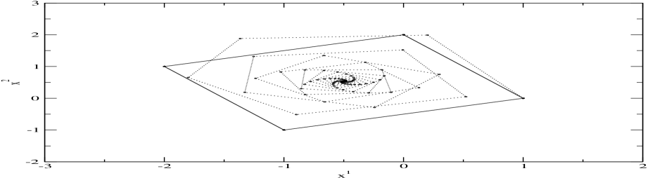
Figure 1: The evolution of the mapping (77) is shown in the $(x^{1},x^{2})$ plane for $\alpha=0$ and $\alpha=0.1$. Circles correspond to positions of the vector ${\bf x}(j)$ for different $j$. Circles connected by the solid and dotted lines represent the cases $\alpha=0$, $\alpha=0.1$, respectively. The angle $\phi_{0}=\pi/2$. Both curves start at the initial value of ${\bf x}(0)$ with coordinates: $x_{i}^{1}(0)=1,\quad x_{i}^{2}(0)=0$. The closed curve corresponding to $\alpha=0$ is a parallelogram where successive values of ${\bf x}(j)$ are situated at vertexes. The curve corresponding to $\alpha=0.1$ is a spiral which ultimately approaches a stationary point with coordinates defined by equation (80).

When $\alpha$ exceeds some value $\alpha_{*}$, this stationary point described above becomes unstable, and the solution exhibits a complicated behaviour, but stochastic growth is not observed (see figure 2).

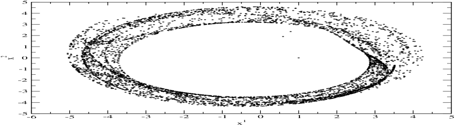
Figure 2: Same as figure 1, but with $\alpha=0.3$. We represent here $5000$ point corresponding to $5000$ iterations of the map (77). The stationary point referred to in the text is unstable in this case, but all points are confined to a small region around it. We have checked for a much larger number of iterations that $|{\bf x}(j)|$ remains bounded. The case is intermediate between attraction to a fixed point and stochastic behaviour.

Finally, when $\alpha$ exceeds some critical value $\alpha_{crit}$, the solution starts to exhibit stochastic behaviour and the mode energy grows on average (see figure 3).

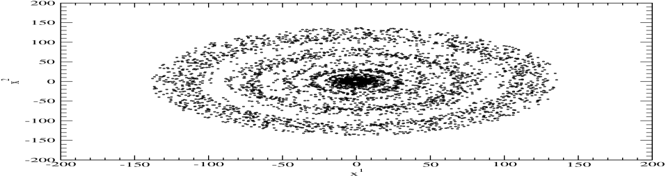
Figure 3: Same as Fig. 1 and Fig. 2, but with $\alpha=0.35$. This value of $\alpha$ approximately corresponds to $\alpha_{crit}$ for $\phi_{0}=\pi/2$ (see Fig. 4). The evolution can be approximately described as a jumping of ${\bf x}(j)$ for successive $j$ between different points on circles. The radius of the circles (proportional to the mode energy) grows on average.

Analytical calculation of $\alpha_{crit}$ is a very complicated mathematical problem so we use a simple numerical method in order to establish the dependence of $\alpha_{crit}$ on $\phi_{0}$. Namely, we iterate the map (77) for a large number $n$ of iterations ($n=5\cdot 10^{4}$, $10^{5}$, $1.5\cdot 10^{5}$) and different values of $\alpha$ and $\phi_{0}$ and find the boundary between stochastic and stable solutions. We solve the system starting with $\alpha=0$, and steadily increase $\alpha$ until $\tilde{E}_{m}(n)$ exceeds the iteration number $n$. The corresponding value of $\alpha$ is associated with $\alpha_{crit}$. We present the dependence of $\alpha_{crit}$ on $\phi_{0}$ in figure 4. One can see from this plot that this value very weakly depends on the iteration number $n$. For our estimates below we use the averaged value of $\alpha_{crit}$

$$\bar{\alpha}_{crit}={1\over 2\pi}\int^{2\pi}_{0}d\phi_{0}\alpha_{crit}\approx 0.67.$$ (87)

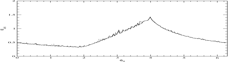
Figure 4: The dependence of $\alpha_{crit}$ on $\phi_{0}$ is shown. The solid, dashed, and dotted lines correspond to $n=1.5\cdot 10^{5}$, $10^{5}$, $5\cdot 10^{4}$, respectively.

One can see from equation (84) that $\alpha\propto a^{5/2}$. Therefore, the stochastic instability always sets in when the semi-major axis $a$ is sufficiently large: $a>a_{st}\equiv a(\alpha=\alpha_{crit})$. To calculate $a_{st}$ explicitly one should specify a particular model of the planet. We calculate it in Section 3.5 below.

The case of rotating planet can be treated by a similar way, but in this case we have a large number of parameters defining the map. The increased number of degrees of freedom in that case is likely to result in decrease of $\alpha_{crit}$ with $\Omega_{r}$. Therefore, we assume that we can use $\alpha_{crit}(\Omega_{r}=0)$ as an approximate upper boundary for the rotating case.

3 Orbital evolution of a massive fully convective planet due to tidal interaction

In this Section we apply the results of the previous section to estimate the effect of tides induced by the central star on the orbital evolution of a massive planet. Consider a planetary system consisting of several massive fully convective planets orbiting a central star at typical separation distances $\sim 1-100Au.$ Suppose that one of these has lost a significant amount of angular momentum (most probably due to interaction with other planets) and has settled into a highly eccentric orbit. The orbital semi-major axis $a$ would then be of the order of ’initial’ separation distance $\sim 1-100Au.$ The minimal separation distance $D_{min}$ is related to the orbital angular momentum per unit of mass $L_{orb}$ through $D_{min}={L^{2}_{orb}\over CM}$ and could be of the order of several stellar radii $R_{*}.$ Situations of this type occur in simulations of gravitating interacting planets (Papaloizou & Terquem 2001, Adams & Laughlin 2003). If close enough approaches to the central star occur, tidal interaction could become important for determining the subsequent orbital evolution of the planet. Below we estimate the relative contribution of stationary and dynamical tides, both exerted by star on planet and planet on star on the orbital evolution. In particular we specify at which separation distances we can expect tidal effects to become significant.

If we assume that the orbital evolution of the planet is determined by tides, while the orbit remains highly eccentric, the total relative change of the orbital angular momentum is much smaller than that of the orbital energy. Thus we may suppose the orbital momentum to be approximately conserved. That leads to the well known result that the ’final’ separation distance of the planet in the ’final’ circular orbit attained at the end of tidal evolution, $D_{fin}$, is twice as large as $D_{min}.$ The shortest observed periods are typically $3$ days for Jovian mass planets around solar type stars (Butler et al 2002). Thus $D_{min}$ is directly related to the observed period $P_{obs}$ of the planet through

$$D_{min}={D_{fin}\over 2}={{(GM)}^{1/3}\over 2}{({P_{obs}\over 2\pi})}^{2/3}=4.36{(P_{3})^{2/3}}({R_{\odot}\over R_{*}})R_{*},$$ (88)

where $R_{\odot}=7\cdot 10^{10}cm$ is the radius of the Sun, and $P_{3}=P_{obs}/(3days)$. Using equation (43) we can also express the parameter $\eta$ in terms of $P_{3}$:

$$\eta=9.1\eta_{0}{({R_{\odot}\over R_{*}})}^{3/2}P_{3},$$ (89)

where

$$\eta_{0}=\sqrt{{m_{pl}\over M}{R^{3}_{*}\over R^{3}_{pl}}}.$$ (90)

For a planet of one Jupiter mass and radius, and a central solar type star, $\eta_{0}\approx 1$.

3.1 The planet model

For a close encounter with the central star occurring with a given distance of closest approach, the strength of tidal effects acting in a planet is sensitive to the magnitude of its radius. This is because the energy gain through the action of dynamical tides decreases exponentially with $\eta$ (see equation(64)) and $\eta\propto R_{pl}^{-3/2}$ is a monotonically decreasing function of the radius of the planet. The energy gain associated with stationary tides being $\propto\eta^{-5}$ also decreases rapidly with $\eta.$

In order to determine the radius, a model for the structure of the planet taking account its history is needed. The radius decreases as the planet cools on a thermal time-scale. Accordingly the model should specify the planetary structure and radius as a function of age.

A young gravitationally contracting planet will be fully convective. If we assume that a turbulent viscosity arising from convection determines the damping rate $\gamma,$ it will be a function of the planet radius and luminosity both of which are functions of time. In this case too, estimation of the importance of tidal interaction requires specification of a time dependent model of the planet.

Because convection is extremely efficient, a fully convective planet can be considered as an isentropic body. For a given composition isentropic models of a given mass can be conveniently parametrised by the planet radius $R_{pl}.$ We have calculated such models using the equation of state of Saumon, Chabrier $\&$ Van Horn (1995) for solar composition neglecting the possible presence of a central small solid core. We have considered the masses $m_{pl}=1M_{J},5M_{J},$ where $M_{J}\approx 1.9\cdot 10^{30}g$ is the mass of Jupiter, with radii in the range $1R_{J}-2.1R_{J}$, where the Jovian radius $R_{J}\approx 7\cdot 10^{9}cm$. The dimensionless density distribution $\tilde{\rho}(r)$ as a function of the dimensionless radius $r/R_{pl}$ is shown in figure 5.

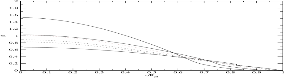
Figure 5: The dimensionless density $\tilde{\rho}$ as a function of the dimensionless radius $r/R_{pl}$. The three solid lines represent $m_{pl}=1M_{J}$ with $R_{pl}=1R_{J}$, $1.5R_{J}$ and $2R_{J}$ respectively. The three dotted lines are for $m_{pl}=5M_{J}$ with $R_{pl}=1.03R_{J}$, $1.54R_{J}$ and $2.06R_{J}.$ The central density grows with $R_{pl}$ for both masses.

Note that the models with larger radii are more centrally condensed, the effect being less prominent for $m_{pl}=5M_{J}.$ Also note the sharp change of the density at $r/R_{pl}\approx 0.82$ for the model with $m_{pl}=1M_{J}$ and $R_{pl}=1R_{J}.$ This is due to the phase transition between molecular and metallic Hydrogen that has been assumed to be first order. This effect is absent for the models with larger radii and larger mass. For these models, the corresponding adiabats have larger entropy and go above the critical point of the Saumon, Chabrier $\&$ Van Horn (1995) equation of state. We calculate the dimensionless frequencies of the fundamental mode $\tilde{\omega}_{00}$ and the dimensionless overlap integrals $\tilde{Q}$ for these models. The results of these calculations are presented in figures 6 and 7.

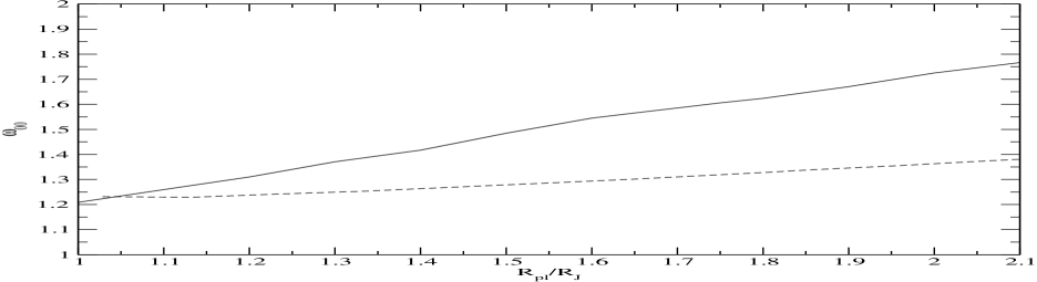
Figure 6: The dimensionless frequency $\tilde{\omega}_{00}$ as a function of the radius of the planet (in units of the Jovian radius). The solid and dashed curves correspond to $m_{pl}=1M_{J}$ and $5M_{J}$ respectively.

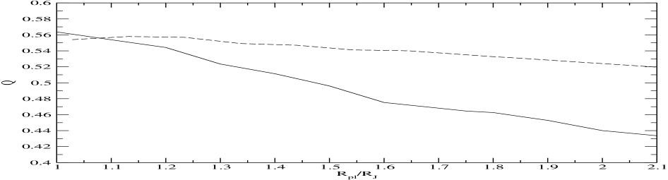
Figure 7: The dimensionless overlap integral $\tilde{Q}$ as a function of the radius of the planet (in units of the Jovian radius). The solid and dashed curves correspond to $m_{pl}=1M_{J}$ and $5M_{J}$, respectively.

The dimensionless frequencies increase, and the dimensionless overlap integrals decrease with $R_{pl}$ these effects being less prominent for $m_{pl}=5M_{J}.$ The value of $\tilde{\omega}_{00}$ for the model with $m_{pl}=1M_{J}$, $R_{pl}=1R_{J}$ is in a good agreement with earlier calculations by Vorontsov (1984), Vorontsov et al (1989), Lee (1993).

The coefficients $\beta$ (equation (19)) determining the frequency splitting due to rotation are close to $0.5$ for all models. Note that this would be exact for an incompressible model.

3.1.1 Evolution of the radius with time

In order to find the dependence of the planetary radius on time, a model of the planetary atmosphere is needed. For a given mass and radius, this is required to determine the luminosity which in turn determines the cooling rate as a function of radius. This is a highly non trivial problem given significant difficulties in calculating molecular opacities for the low temperatures and high densities of interest. Other complications may arise from the possible presence of clouds of different condensed chemical species, etc. We use the relationship between radius and luminosity and hence the planetary age calculated by Burrows et al (1997) in the framework of a non-gray atmospheric model. The results of these calculations are shown in figures 8 and 9. As one can see from figure 8, the radius of the planet decreases from $\sim 1.7R_{J}$ at $t=10^{6}yr$ to $\sim R_{J}$ at $t\sim 8\cdot 10^{9}yr$. Note that this result is close to that obtained by Graboske et al (1975) for their model of the evolution of Jupiter.

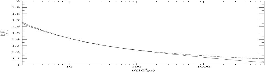
Figure 8: The radius of the planet (in units of the Jovian radius) as a function of time (in units $10^{6}yr$). The solid and dashed curves correspond to $m_{pl}=1M_{J}$, $5M_{J}$, respectively. Note that the dependence of radius on time is rather similar for both models.

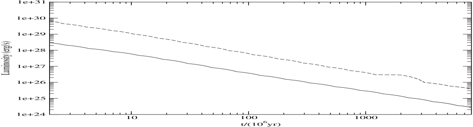
Figure 9: The internal luminosity of the planet (erg/s) as a function of time (in units $10^{6}yr$). The solid and dashed curves correspond to $m_{pl}=1M_{J}$ and $5M_{J}$, respectively. The more massive planet is more than ten times more luminous.

We here point out that tidal heating might significantly delay or even reverse the cooling of the planet. This effect is not considered here as we focus on the initial stages of tidal evolution and so do not solve a self-consistent problem for the thermodynamics of a planet with an energy source due to tidal heating.

3.1.2 The convective time scale

An important time scale is the characteristic time associated with convective eddies $t_{c}$. These will be of large scale in the fully convective planetary interior. This characteristic time has been estimated by Zahn (1977) to be

$$t_{c}\sim t_{zh}\equiv{\left({m_{pl}R_{pl}^{2}\over\dot{E}_{th}}\right)}^{1/3},$$ (91)

where $\dot{E}_{th}$ is the energy transport rate due to convection. This is comparable to the total luminosity. The dependence of $t_{zh}$ on time is shown in figure 10.

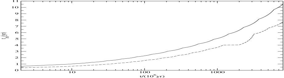
Figure 10: The convective time scale $t_{zh}$ as a function of time (in units $10^{6}yr$). The solid and dashed curves correspond to $m_{pl}=1M_{J}$ and $5M_{J}$ respectively. Note that this time scale is the same order of magnitude for both masses.

One can see from figure 10 that $t_{zh}$ grows with time from $\sim 0.5yr$ at an age of $10^{6}yr$ to $\sim 10yr$ at an age of $10^{9}yr.$ Assuming that dissipation is determined by a turbulent viscosity that acts like an anomalously large molecular viscosity, we can express the dissipation rate given by equation (20) as

$$\gamma={\lambda(m_{pl},R_{pl})\over t_{zh}},$$ (92)

where the coefficient $\lambda(m_{pl},R_{pl})\sim 10^{-2}-10^{-1}$ for different models of the planet.

In fact the dissipation rate may be much smaller than that given by equation (92). This is because as the largest convective eddies have the size of order of the mixing length, which in the deep interior is on the order of the local radius, they can only fully distribute the energy and momentum of the hydrodynamical motion induced by the tidal field on the mixing length scale in a time $\sim t_{c}\gg t_{f}$, where $t_{f}\sim 1day$ is the characteristic time associated with tidal forcing (Goldreich $\&$ Nicholson 1977). This leads to a correction factor $\sim{({t_{f}\over t_{c}})}^{n}$ in equation (92). In the literature it has been suggested that $n$ may be equal either to $2$ (e.g. Goldreich $\&$ Nicholson 1977) or to $1$ (Zahn 1989). Neglecting the contribution of layers close to the surface of the planet, we adopt $t_{c}\sim t_{zh}$, and modify the expression (92) taking into account the correction factor so obtaining

$$\gamma_{m}\sim{({t_{f}\over t_{zh}})}^{n}({\lambda(m_{pl},R_{pl})\over t_{zh}}).$$ (93)

3.2 Orbital evolution due to quasi-static tides

We show here that in our approximation, the time scale for orbital evolution due to quasi-static tides of a planet in a highly eccentric orbit is exceedingly large. In order to make an estimate of the evolution time scale we assume the planet to be rotating at its ’equilibrium’ angular velocity $\Omega_{ps}$ and therefore evolving at fixed orbital angular momentum. This is reasonable on account of the low moment of inertia associated with the planetary rotation compared to that of the orbit. The planet in a highly eccentric orbit can be considered to have a sequence of impulsive energy gains occurring at periastron passage. Each energy gain $\Delta E_{st}$ is given by equation (47). Since the energy gain depends on orbital parameters only through the dependence of $\eta$ on the minimum separation distance and for highly eccentric orbits the minimum separation distance is determined by the value of the orbital angular momentum, the energy gain $\Delta E_{st}$ is constant during the orbital evolution.

The law of energy conservation gives

$${\Delta E_{st}\over P_{orb}}+{GMm_{pl}\over 2a^{2}}\dot{a}=0,$$ (94)

where $a$ is the semi-major axis, and $P_{orb}=2\pi\sqrt{{a^{3}\over GM}}$ is the orbital period (also see equation (66)). From equation (94) we obtain the evolution equation for the semi-major axis in the form

$${\dot{a}\over a}=-{1\over t_{ev}},$$ (95)

with

$$t_{ev}=\pi\left({GMm_{pl}\over a\Delta E_{st}}\right)\sqrt{{a^{3}\over GM}}.$$ (96)

It is convenient to introduce a scale $a_{*}$ defined by the condition that the planetary internal energy is approximately equal to the orbital energy in the form

$$a_{*}={M\over m_{pl}}R_{pl}\approx 7\cdot 10^{12}\times\left({R_{pl}\over R_{J}}\right)\left({MM_{J}\over M_{\odot}m_{pl}}\right)cm.$$ (97)

Using this we can express $t_{ev}$ in the form

$$t_{ev}={E_{pl}\over 2\Delta E_{st}}{\left({a\over a_{*}}\right)}^{1/2}P_{*},$$ (98)

where

$$P_{*}\equiv P_{orb}(a=a_{*})=0.32\left({M\over M_{\odot}}\right){\left({M_{J}R_{pl}\over m_{pl}R_{J}}\right)}^{3/2}yr.$$ (99)

One can easily estimate from equation (98) that $t_{ev}$ is very large. Indeed, $\Delta E_{st}/E_{pl}$ can be estimated from equation (47) to be

$$\Delta E_{st}/E_{pl}\sim{\tilde{\gamma}\over\eta^{5}},$$ (100)

where we have assumed that $\tilde{\omega}_{00}$ and $\tilde{Q}\sim 1$. Taking into account that $t_{zh}\sim 1-10yr$, and $\lambda\sim 10^{-2}$, we find $\tilde{\gamma}$ using equation (92) to be $\tilde{\gamma}\mathrel{\hbox to0.0pt{\lower 3.0pt\hbox{$\mathchar 536\relax$}\hss}\raise 2.0pt\hbox{$\mathchar 316\relax$}}10^{-6}$. Since $\eta\sim 10$ in our problem, we obtain $\Delta E_{st}/E_{pl}\mathrel{\hbox to0.0pt{\lower 3.0pt\hbox{$\mathchar 536\relax$}\hss}\raise 2.0pt\hbox{$\mathchar 316\relax$}}10^{-11}$, and thus

$$t_{ev}\sim 10^{11}{({a\over a_{*}})}^{1/2}{({M_{J}\over m_{pl}})}^{3/2}yr.$$

More accurately, we can take into account the fact that $\Delta E_{st}$ depends on several quantities which are functions of time, making in turn $t_{ev}$ a function of time also. We show the dependence of $t_{ev}$ on $t$ in figure 11 assuming that $\eta=10$, $a=a_{*}$ and the damping rate is given by equation (92).

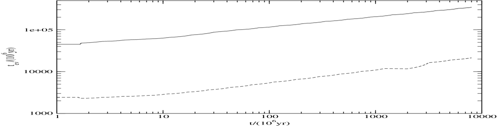
Figure 11: The time scale of evolution due to quasi-static tides, $t_{ev},$ (in units of $10^{6}$yr) as a function of time ( in the same units) for $a=a_{*}$. The solid and dashed curves correspond to $m_{pl}=1M_{J}$ and $5M_{J}$ respectively.

One can see from figure 11 that the time scale of orbital evolution due to quasi-static tides is very large, being typically the order of $\sim 10^{9}-10^{10}yr$ for $m_{pl}=5M_{J}$, and order of magnitude larger for $m_{pl}=M_{J}$. In fact, the evolution time may even be much larger if we take into account the correction factor to the damping rate (equation (93)). Therefore, if we assume that the viscous damping rate is determined by convective turbulent viscosity, the evolution of a planet’s orbit due to quasi-static tides appears to be impossible for semi-major axes $\mathrel{\hbox to0.0pt{\lower 3.0pt\hbox{$\mathchar 536\relax$}\hss}\raise 2.0pt\hbox{$\mathchar 318\relax$}}0.1Au$.

We have also made simple estimates of the evolution due to quasi-static tides acting in a star with a solar-like convective envelope and found that the rate of evolution of a planet orbit with orbital parameters typical of our problem due to tides in the star also seems to be rather weak.

3.3 Dynamic Tides in the star versus Dynamic Tides in the planet

In order to estimate effects due to dynamic tides in the star we model it as a simple $n=3$ polytrope and calculate the energy gain due to dynamic tides, $\Delta E_{ns*}$ using the expressions given by PT. Our results agree well with those of Lee and Ostriker (1986), but we include the contribution of a larger number of $g$ modes to $\Delta E_{ns*}$ and therefore obtain a slightly larger value of $\Delta E_{ns*}$ for large separation distances. It is important to note that the quantity $\eta_{*}$ associated with tides in the star is different from that associated with the planet (equation (43)) being given by the expression (PT)

$$\eta_{*}={({D_{min}\over R_{*}})}^{3/2}\approx 9{({R_{\odot}\over R_{*}})}^{3/2}P_{3}.$$ (101)

In order to show the values of $\Delta E_{ns}$ and $\Delta E_{ns*}$ in the same figure, we use the orbital period $P_{obs}$ as independent variable. These quantities are represented in figure 12 and figure 13 for $m_{pl}=1M_{J}$ and $m_{pl}=5M_{J}$ respectively.

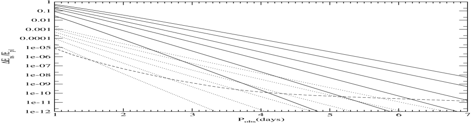
Figure 12: The energy gains $\Delta E_{ns}$, $\Delta E_{ns*}$ obtained by the planet (solid and dotted curves) and by the star (the dashed curve) after ’the first’ periastron fly-by. The six solid curves correspond to a non-rotating planet ($\Omega_{r}=0$) and represent the expression 59) for the six different values $R_{pl}=1R_{J}$, $1.2R_{J}$, $1.4R_{J}$, $1.6R_{J}$, $1.8R_{J}$ and $2R_{J}$. Obviously, the curves corresponding to larger values of $R_{J}$ have larger values of $\Delta E_{ns}$. The six dotted curves represent the same quantities but calculated for a planet with ’critical’ rotation rate $\Omega_{r}=\Omega_{crit}$. They are given by the expression (65).

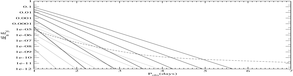
Figure 13: Same as 12, but calculated for $m_{pl}=5M_{J}$.

One can see from figure 12 that the energy gain $\Delta E_{ns}$ sharply decreases with $P_{obs}$. However, in most cases $\Delta E_{ns}\gg\Delta E_{ns*}$ at $P_{obs}\sim 1day$. For a non-rotating planet with $m_{pl}=1M_{J}$ tides in the planet are dominant for all interesting values of $\Delta E_{ns}$: $\Delta E_{ns}/E_{pl}\mathrel{\hbox to0.0pt{\lower 3.0pt\hbox{$\mathchar 536\relax$}\hss}\raise 2.0pt\hbox{$\mathchar 318\relax$}}10^{-10}-10^{-9}$. Even when the planet rotates at $\Omega=\Omega_{crit}$ (corresponding to minimal possible energy gain for a given $P_{obs}$, see equation (65)), the tides in the planet dominate for models with $R_{pl}>1.4R_{J}$. The planet with $m_{pl}=5M_{J}$ is more dense, and the role of tides operating in the planet is less prominent. In that case the curves corresponding to ’critical’ rotation are situated below the curve corresponding to the tides in the star for almost the whole range of $P_{obs}.$

3.4 Orbital evolution due to Dynamic Tides

If we assume that either each impulsive energy transfer to the planet is dissipated before the next, or that the condition of the stochastic build-up of mode energy is fulfilled, in either case we can write the equation for the evolution of the semi-major axis due to dynamical tides in a form similar to equation (95)

$${\dot{a}_{10}\over a_{10}}=-{1\over t_{10}(t)\sqrt{a_{10}}},$$ (102)

where $a_{10}=a/10Au.$ The time

$$t_{10}=7.4\cdot 10^{8}\left({MM_{J}\over M_{\odot}m_{pl}}\right)\left({R_{pl}\over R_{J}}\right)\epsilon_{ns}^{-1}yr,$$ (103)

is the ’local’ evolution time for the orbit with semi-major axis $\sim 10Au\gg a_{*}$ and $\epsilon_{ns}=10^{9}(\Delta E_{ns}+\Delta E_{ns*})/E_{pl}.$ We would like to stress that if the tidal energy transfer process is in the stochastic regime, equation (102) must be understood as describing the evolution of an average value of $a$ (see previous Section).

Equation(102) can be integrated to give

$$a_{10}=a_{in}\left(1-{1\over 2\sqrt{a_{in}}}\int^{t}_{t_{in}}{dt^{{}^{\prime}}\over t_{10}(t^{{}^{\prime}})}\right)^{2}=a_{in}\left(1-{\sqrt{a_{cap}\over a_{in}}}\right)^{2},$$ (104)

where $a_{in}$ and $t_{in}$ are the ’initial’ values of the semi-major axis (in units of $10Au$) and the initial time respectively. The quantity

$$a_{cap}={1\over 4}\left(\int^{t}_{t_{in}}{dt^{{}^{\prime}}\over t_{10}(t^{{}^{\prime}})}\right)^{2}$$ (105)

defines the typical ’capture’ scale. This is because at any moment of time $t,$ the orbits with initial values of the semi-major axes $a_{in}<a_{cap}(t)$ have changed their semi-major axes significantly before the time $t$ and the orbits with $a_{in}>a_{cap}(t)$ have $a\sim a_{in}.$

We can define the evolution time more accurately as the time when the term in brackets in equation (104) is equal to zero. Thus

$${1\over 2\sqrt{a_{in}}}\int^{t_{ev}}_{t_{in}}{dt^{{}^{\prime}}\over t_{10}(t^{{}^{\prime}})}=1.$$ (106)

Obviously, this time is a function of $a_{in}$ and $t_{in}$. For a constant value of $t_{10},$ $t_{ev}\approx 2\sqrt{a_{in}}t_{10}.$

The results of calculation of $t_{ev}$ and $a_{cap}$ are presented in figures 14-15. For our calculations we assume that $t_{in}\sim 10^{6}yr$ and note that results can be easily generalised for other values of $t_{in}$. In figure 14 we show results of calculations of $t_{ev}$ for the two planetary masses ($m_{pl}=1M_{J},5M_{J}$), and two values of the angular velocity of the planet ($\Omega_{r}=0,\Omega_{crit}$). The orbit of non-rotating $1M_{J}$ planet can be evolved by dynamical tides in a time $\mathrel{\hbox to0.0pt{\lower 3.0pt\hbox{$\mathchar 536\relax$}\hss}\raise 2.0pt\hbox{$\mathchar 316\relax$}}10^{10}yr$ for $P_{obs}<P_{max}\sim 5days$ (see the lower solid curve in figure 14 ). The orbit of a $1M_{J}$ planet with $\Omega_{r}=\Omega_{crit}$ has $P_{max}\approx 4days$. Orbits of non-rotating and rotating planets with $m_{pl}=5M_{J}$ have $P_{max}\sim 5-6days.$ In that case the evolution is determined by dynamical tides in the star for $P_{obs}\mathrel{\hbox to0.0pt{\lower 3.0pt\hbox{$\mathchar 536\relax$}\hss}\raise 2.0pt\hbox{$\mathchar 318\relax$}}3days$ (both dashed curves almost coincide in figure 14 for $P_{obs}\mathrel{\hbox to0.0pt{\lower 3.0pt\hbox{$\mathchar 536\relax$}\hss}\raise 2.0pt\hbox{$\mathchar 318\relax$}}3days$).

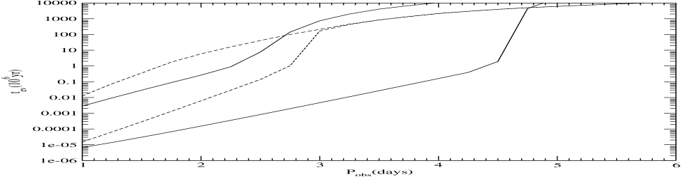
Figure 14: The time $t_{ev}$ (see equation (106) for definition) is shown as a function of $P_{obs}.$ The solid and dashed curves correspond to $m_{pl}=1M_{J},5M_{J}$, respectively. The lower and upper curves of the same type correspond to ($\Omega_{r}=0,\Omega_{crit}$). We choose $a_{in}=10Au$ for all curves.

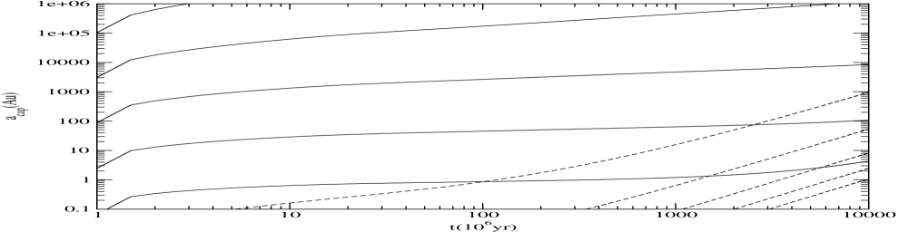
Figure 15: The dependence of $a_{cap}$ (in $Au$ ) on time (in units $10^{6}yr)$. The solid and dashed curves correspond to $\Omega_{r}=0,\Omega_{crit}$. The five curves of the same type correspond to different $P_{obs}=3,3.5,4,4.5,5day$. The lower curves correspond to larger periods.

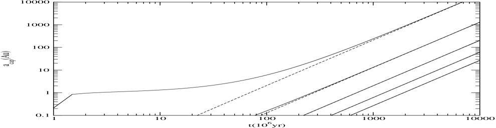
Figure 16: Same as figure 15, but for $m_{pl}=5M_{J}$. Note that all curves except the curve corresponding to $\Omega_{r}=0$ and $P_{obs}=3days$ are close to straight lines. Also, curves with the same period $P_{obs}$ are close to each other. This is due to the fact that the orbital evolution is mainly determined by dynamic tides in the star for $m_{pl}=5M_{J}$.

One can see from figure (14) that for a non-rotating planet and $P_{obs}\sim 1day$, $t_{ev}$ is about a few years and is of order of the orbital period. Such a fast tidal evolution may possibly lead to disruption of the planet (see also Discussion).

3.5 Onset of the stochastic instability

Finally, let us discuss the condition leading to stochastic build-up of the mode energy. From the results of Section 2.9 it follows that the stochastic instability sets in when the orbital semi-major axis is sufficiently large: $a\mathrel{\hbox to0.0pt{\lower 3.0pt\hbox{$\mathchar 536\relax$}\hss}\raise 2.0pt\hbox{$\mathchar 318\relax$}}a_{st}$, where $a_{st}$ can be expressed in term of the parameter $\bar{\alpha}_{crit}$ (see equation (87)) using equation (84)

$$a_{st}=({\alpha_{crit}E_{pl}\over 6\pi\tilde{\omega}_{00}(\Delta E_{ns}+\Delta E_{ns*})})^{2/5}({M\over m_{pl}})^{3/5}R_{pl}\approx 30.8(\tilde{\omega}_{00}\epsilon_{ns})^{-2/5}({M_{J}\over m_{pl}})^{3/5}({R_{pl}\over R_{J}})Au,$$

and we use the value $\bar{\alpha}_{crit}=0.67$ on the right hand side.

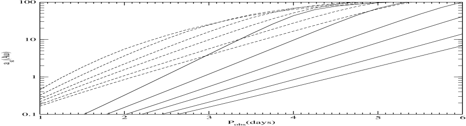
Figure 17: The dependence of $a_{st}$ (in $Au$) on $P_{obs}$ (in days). The solid and dashed curves correspond to $\Omega_{r}=0,\Omega_{crit}$. Six curves of the same type correspond to different $R_{pl}/R_{J}=1,1.2,1.4,1.6,1.8,2$. The smaller values of $a_{st}$ correspond to larger values of $R_{pl}$.

The result of calculation of $a_{st}$ for a $1M_{J}$ planet is shown in figure 17. One can see from this that the ’stochastic scale’ is of the order of the scales of interest $\sim 0.1-100Au$, with larger values corresponding to the planet with $\Omega_{r}=\Omega_{crit}$.

Accordingly, the stochastic build-up of mode energy may be difficult to achieve for planets rotating at the critical rate (see however Section 4). For non-rotating planets this problem is much less severe. For example, for the non-rotating planet with $R_{pl}\approx 1.6R_{J}$ and $P_{obs}\sim 4days$ we have $a_{st}\approx 2Au$ (figure 17). Thus an orbit with ’initial’ value of the semi-major axis $\sim 10Au$ can be evolved by stochastic tides in a time $t_{ev}\sim 10^{5}yr$ (see figure 14) which is much smaller than the planet’s cooling time $\sim 10^{6}yr$. Therefore dynamical tides can significantly change the semi-major axes of non-rotating planets with parameters appropriate for observed systems.

It is instructive to compare the analytic condition (107) with the results of numerical experiments (Mardling 1995 a, Mardling $\&$ Aarseth 2001). Madling (1995)a and Marldling $\&$ Aarseth (2001) define the boundary between stochastic and regular regimes of tidal evolution as a curve $D_{min}^{crit}(e)$ on the plane $(e,D_{min})$, where $e$ is the eccentricity of the orbit. The stochastic region is situated below this curve. For a $n=1.5$ polytrope Mardling (1995)a obtains: $D_{min}^{crit}(e\approx 0.9)\approx 3.75$, $D_{min}^{crit}(e\approx 0.95)\approx 4.2$, $D_{min}^{crit}(e\approx 0.99)\approx 4.5$, where the minimal separation or pericentre distance is expressed in units of stellar radii. Assuming that the mass ratio is equal to one and using the values $\tilde{\omega}_{00}\approx 1.45$ and $\tilde{Q}\approx 0.5$ (Lee $\&$ Ostriker 1986) we can obtain a similar curve $\tilde{D}_{min}^{crit}(e)$ from our criterion (107). This curve is qualitatively similar to $D_{min}^{crit}(e)$. We have $\tilde{D}_{min}^{crit}(e\approx 0.9)\approx 3.1$, $\tilde{D}_{min}^{crit}(e\approx 0.95)\approx 3.4$, $\tilde{D}_{min}^{crit}(e\approx 0.99)\approx 4$. Our curve lies below $D^{crit}_{min}(e)$ on the plane $(e,D_{min})$ and for a specified value of $e>0.9$ gives a value of $D_{min}$ that is $10-20$ percent smaller. A possible reason for this difference is the neglect of higher order terms in the tidal potential and the contribution of p-modes in our treatment of the problem which would enhance the tidal interaction and lead to larger values of $D_{min}$.

We do not discuss the condition for stochastic build-up of mode energy for planets with $m_{pl}=5M_{J}$. As was shown above, the semi-major axis of such a planet is mainly evolved as a result of dynamical tides in the star. These tides mainly excite $f$ and low order $g$ modes. These modes may interact effectively with high $l$ $g$-modes due to resonant non-linear mode-mode interaction (Kumar $\&$ Goodman 1996). Kumar and Goodman estimated the energy in tidally excited modes needed to be larger than $\sim 10^{36}ergs$ for the resonant parametric instability to occur. This is of the order of the energy obtained by the star after a fly-by of a $5M_{J}$ planet with minimal separation distances typical of our problem. The parametric instability may not only damp effectively the tidally exited modes but also lead to phase changes in these modes thus facilitating the stochastic build-up of mode energy in the star. However, this possibility needs further investigation.

4 Discussion and Conclusions

In this paper we have developed a theory of the tidal interaction between a central star and a massive convective planet moving on a highly eccentric orbit. We showed that it is possible to develop a self-consistent perturbative approach to the theory of disturbances induced in a slowly rotating planet by tidal interaction by regarding them as resulting from a sequence of impulsive interactions occurring at periastron (e.g.. Press & Teukolsky 1977). We obtained contributions to the energy and angular momentum exchanged during periastron passage from both quasi-static and dynamic tides that were derived from the same set of governing equations. Quasi-static tides require the existence of dissipative processes in order to produce net energy and angular momentum transfers from the orbit. However, dynamic tides may do this through the excitation of normal modes.

We found that if the planet was initially non rotating, dynamic tides would transfer angular momentum to it until a ’critical’ equilibrium prograde rotation rate, $\Omega_{crit},$ was attained. This is defined by the condition that dynamic tides acting on a planet rotating with the angular velocity $\Omega_{crit}$ at periastron result in no net angular momentum transfer and hence do not change the rotation rate of the planet . . We found that the rotation rate of the planet which minimised the energy gained as a result of a periastron passage was also equal to $\Omega_{crit}.$ We showed further that this rotation rate depends on the periastron distance between planet and star and that it can be larger than the similar equilibrium ’pseudo-synchronisation’ rotation rate $\Omega_{ps}$ obtained through the action of quasi-static tides. In fact, for sufficiently small periastron distances, our analysis indicates that $\Omega_{crit}$ can attain values of the order of the planet characteristic frequency $\Omega_{*}=\sqrt{{Gm_{pl}\over R_{pl}^{3}}}$ so that a planet rotating with $\Omega_{r}\sim\Omega_{crit}$ may be near to rotational break up. However, the analysis assumed slow rotation. Thus this issue requires further investigation and consideration of the tidal interaction when the planet rotates rapidly.

We examined the consequences of multiple periastron passages and energy exchanges, which, because they occur impulsively at periastron, could be modelled with a simple algebraic map. Multiple encounters can lead to a stochastic build-up of the energy contained in normal modes of oscillation (see Mardling 1995 a,b). We found a simple criterion for the instability of the dynamical system to such a stochastic build-up.

Our results can be applied not only to recently discovered planetary systems containing a star and massive planet, but also in the much more general context of the tidal interaction of a solar type star with a fully convective object or the tidal interaction between two fully convective objects (such as e.g. low mass stars, brown dwarfs, etc.).

We focused on the problem of the tidal evolution of a planet orbiting around a star on a highly eccentric orbit. Such a configuration might be produced as a result of gravitational interaction in a many planet system (e.g. Weidenschilling & Mazari 1996; Rasio & Ford 1996; Papaloizou & Terquem 2001; Adams & Laughlin 2003).

The minimum periastron distance of the orbit was assumed to be $\mathrel{\hbox to0.0pt{\lower 3.0pt\hbox{$\mathchar 536\relax$}\hss}\raise 2.0pt\hbox{$\mathchar 318\relax$}}4$ stellar radii corresponding to a final period $P_{obs}$, after an (assumed) stage of tidal circularization at constant orbital angular momentum, exceeding about $3days$. The initial semi-major axis $a$ was assumed to be of the order of some ’typical’ planet separation distance ranging from $1-100Au.$

We made some simple estimates of the possible tidal evolution of the orbit. We used a realistic model of the planet taking into account the fact that the radius and luminosity decrease with age as the planet cools. We first showed that quasi-static tides cannot account for a significant tidal evolution when the semi-major axes exceed $\sim 0.1Au$. However, dynamical tides can in principle lead to a large decrease of the semi-major axis and circularize the orbit on a time-scale $t_{ev}\mathrel{\hbox to0.0pt{\lower 3.0pt\hbox{$\mathchar 536\relax$}\hss}\raise 2.0pt\hbox{$\mathchar 316\relax$}}10^{9}-10^{10}yr$.

Note that for simplicity we did not take into account possible gravitational interaction of the planet with orbital parameters evolving due to tides with other planets in the planetary system. The possible characterization of this interaction could be decribed as follows. If the characteristic time of gravitational interaction $t_{gr}$ is smaller than $t_{ev}$ the orbital evolution would be mainly determined by the interaction with other planets. The interaction time $t_{gr}$ may increase significantly if the planet is scattered into a highly eccentric orbit by another planet that is itself ejected or scaterred to large distance. In addition $t_{ev}$ sharply decreases with decrease of orbital semi-major axis. For a sufficiently small semi-major axis one would expect that $t_{ev}<t_{gr}$ and the orbital evolution to be mainly determined by tides. Such a formulation of the problem is similar to the well-known loss cone problem in physics of stellar systems around super-massive black holes and is sufficiently complex to require analysis by numerical means.

In a fully convective planet dynamic tides cause the excitation of mainly the $l=2$ fundamental mode of pulsation. This mode has a period that is typically much smaller than a characteristic time of periastron passage corresponding to a typical orbital period $\sim P_{obs}.$ The amount of energy and angular momentum gained at periastron due to dynamical tides decreases exponentially with $P_{obs}.$ Therefore, the evolution time $t_{ev}$ is very sensitive to the value of $P_{obs}.$ Orbits of planets with mass $\sim 1M_{J}$ can be effectively circularized by the tides for final orbital periods $P_{obs}\sim 3-4days$ corresponding to the shortest observed periods in extra-solar planetary systems. However, the contribution of dynamic tides to the orbital circularization rate does not seem to be effective for larger periods $P_{obs}\mathrel{\hbox to0.0pt{\lower 3.0pt\hbox{$\mathchar 536\relax$}\hss}\raise 2.0pt\hbox{$\mathchar 318\relax$}}5days$. These results appear to be consistent with the observational result that the orbits of extra-solar planets are nearly circular (eccentricity $<0.06$) for periods $P_{obs}\mathrel{\hbox to0.0pt{\lower 3.0pt\hbox{$\mathchar 536\relax$}\hss}\raise 2.0pt\hbox{$\mathchar 316\relax$}}5days$. Dynamic tides raised in the star are not important for the orbital evolution of $1M_{J}$ planets. However, for planets with larger mass $\mathrel{\hbox to0.0pt{\lower 3.0pt\hbox{$\mathchar 536\relax$}\hss}\raise 2.0pt\hbox{$\mathchar 318\relax$}}5M_{J}$, the stellar dynamic tides are significant.

There are at least three possible problems with the scenario of tidal circularization we have discussed here. Firstly, dynamical tides can only transfer energy from the orbit to the planet effectively only for sufficiently large orbital semi-major axes $a>a_{st}.$ For orbits with $a<a_{st}$, stochastic instability leading to the energy transfer is ineffective so that the orbital evolution would instead be determined by the decay time of the fundamental mode of oscillation. This would lead to a very large circularization time-scale. This difficulty can possibly be overcome in the following way. Suppose that the planet starts its tidal evolution with $a>a_{st}.$ When $a$ has decreased to $a\sim a_{st}$, assuming little dissipation, a significant energy $\sim{GMm_{pl}\over a_{st}}$ would be contained in the oscillations of the planet. Eventually non linear effects should start to cause dissipation of this energy and a significant expansion of the radius which in turn produces a significant increase in the energy transfer from the orbit to the planet by tides. This could produce a form of tidal runaway (e.g.. Gu, Lin $\&$ Bodenheimer 2003) until possibly a balance between dissipation of energy due to nonlinear effects and tidal injection is attained. In this situation, a condition of effective stochastic instability may be fulfilled all the way down to the final quasi-circular orbit. Self-consistent calculations taking into account the non-linear effects of tidal heating on the structure of the planet are needed in order to evaluate this possibility .

On the other hand, if the dynamical tides operate effectively on scales $\ll a_{st}$ there is enough energy exchanged to destroy the planet. Indeed if the planet semi-major axis is smaller than $a_{*}={M\over m_{pl}}R_{pl}\approx 7\cdot 10^{12}({M_{J}\over m_{pl}})cm$, the magnitude of the orbital energy becomes larger than the internal energy of the planet. Therefore, in order to settle onto a tight circular orbit around the star, short period planet must dissipate and radiate away an amount of energy which is much larger than its internal energy. This issue needs to be discussed in the context of a non-linear analysis of the orbital evolution.

Finally, in our approximations, the influence of dynamical tides decreases exponentially with $P_{obs}$ and the tidal evolution as well as initial conditions of the problem are likely to be stochastic. Under such conditions there may exist other planets in the same system which have failed to circularize their orbits and have very high orbital eccentricities at the present time (the difference $1-e\sim 10^{-3}-10^{-4}$). This difficulty may appear less significant when one considers the possible contribution of other non-standard long period modes of oscillation. The energy transferred to these modes could lead to tidal evolution at larger separation distances (corresponding to $P_{obs}\mathrel{\hbox to0.0pt{\lower 3.0pt\hbox{$\mathchar 536\relax$}\hss}\raise 2.0pt\hbox{$\mathchar 318\relax$}}5$).

There are at least two possible candidates for such modes. Firstly, there is a low-frequency mode associated with the first order phase transition between molecular and metallic Hydrogen (Vorontsov 1984, Vorontsov, Gudkova and Zharkov 1989). This mode has a period approximately twice as long as the period of the fundamental mode. However this mode is probably not important for our problem. As we have mentioned before the phase transition is absent in hot young planets. Also, this mode disappears when the time scale of the transition of one phase to another is smaller than the period of the mode (Vorontsov 1984). Another very interesting possibility is to consider the inertial modes associated with rotation of the planet (e.g. Papaloizou $\&$ Pringle 1978). The modes have very low frequency and therefore their excitation does not decrease exponentially with distance. The density perturbation associated with these modes is small being of order $\Omega_{r}^{2}.$ However, the contribution of these modes to the energy gained from the orbit may be significant for large values of $P_{obs}$ where the contribution of the fundamental mode is exponentially small. We will to consider the excitation of these modes by dynamical tides in our future work.

Appendix A Derivation of the explicit expression for the damping rate

In order to obtain equation (20) from equation (15), we need to evaluate the following expression

$$a={1\over 2}\int d\Omega\sigma^{*\beta}_{\alpha}\sigma^{\alpha}_{\beta},$$

where $\sigma^{*\beta}_{\alpha}$ is related to the displacement through equation (16) and integration is performed over the solid angle $\Omega$. We assume an isentropic condition leading to a circulation free displacement such that $\nabla\times\mbox{\boldmath$\xi$}=0$ is fulfilled. We may then introduce a displacement potential $\Phi$ such that ${\mbox{\boldmath$\xi$}}=\nabla\Phi$, and rewrite (A1) in terms of it so obtaining

$$a=2\int d\Omega(\Phi^{*}_{,\alpha\beta}\Phi_{,\alpha\beta}-{1\over 3}\Delta\Phi^{*}\Delta\Phi).$$

We use the identity

$$\Phi^{*}_{,\alpha\beta}\Phi_{,\alpha\beta}={1\over 2}(\Delta(\Phi^{*}_{,\alpha}\Phi_{,\alpha})-(\Phi^{*}_{,\alpha}\Delta\Phi_{,\alpha}+\Phi_{,\alpha}\Delta\Phi^{*}_{,\alpha})),$$

to bring (A2) in the form

$$a=\int d\Omega(\Delta(\Phi^{*}_{,\alpha}\Phi_{,\alpha})-(\Phi^{*}_{,\alpha}\Delta\Phi_{,\alpha}+\Phi_{,\alpha}\Delta\Phi^{*}_{,\alpha})-{2\over 3}\Delta\Phi^{*}\Delta\Phi)$$

$$=\int d\Omega(\Delta(\mbox{\boldmath$\xi$}\cdot\mbox{\boldmath$\xi$}^{*})-\mbox{\boldmath$\xi$}^{*}\cdot\nabla(\nabla\cdot\mbox{\boldmath$\xi$})-\mbox{\boldmath$\xi$}\cdot\nabla(\nabla\cdot\mbox{\boldmath$\xi$}^{*})-{2\over 3}(\nabla\cdot\mbox{\boldmath$\xi$})(\nabla\cdot\mbox{\boldmath$\xi$}^{*})).$$

Now we substitute equation (12) into (A3), use the relation (13) and the known properties of the vector functions to obtain

$$a=2\{{2\over 3}(\xi_{R}^{{}^{\prime}}-{\xi_{R}\over r}+{L^{2}\over 2}{\xi_{S}\over r})^{2}+{1\over r^{2}}(2(\xi_{R}-{L^{2}\over 2}\xi_{S})^{2}+(L^{2}-2)\xi_{R}^{2}+L^{2}{(\xi_{R}-\xi_{S})}^{2})\},$$

where $L^{2}=l(l+1)$. Note that (A4) cannot be used for $l=0$. Multiplying equation (A4) on ($r^{2}\rho\nu$), setting $l=2$ ($L^{2}=6$) and integrating the result over $r$ we get equation (20).

References

- [] Adams, F.C., Laughlin, G., 2003, Icarus, in press
- [] Alexander, M. E., 1973, Astrophys. Space Sci., 23, 459
- [] Boss, A.,P., 2002, ApJ, 576, 462
- [] Burrows, A., Marley, M., Hubbard, W. B., Lunine, J. L., Guillot, T., Saumon, D., Freedman, R., Sudarsky, D., Sharp, C., 1997, ApJ, 491, 856
- [] Butler, R. P, Marcy, G. W., Vogt, S. S., Tinney, C. G., Jones, H. R. A., McCarthy, C., Penny, A. J., Apps, K. C., Brad, D., 2002, ApJ, 578, 565
- [] Chandrasekhar, S., 1964, ApJ, 139, 664
- [] Christensen-Dalsgaard, J., 1998, Lecture Notes on Stellar Oscillations, Forth Edition, Dept. of Physics and Astronomy, University of Aarhus, http://astro.phys.au.dk/ jcd/oscilnotes/
- [] Eggleton, P. P., Kiseleva, L. G., Hut, P., 1998, ApJ, 499, 853
- [] Friedman, J. L., Schutz, B. F., 1978, ApJ, 221, 937
- [] Goldreich, P., Nicholson, P. D., Icarus 1977, 30, 301
- [] Graboske, H. C., Pollack, J. B., Grossman, A. S., Olness, R. J., 1975, ApJ, 199, 265
- [] Gu, P., Lin, D., Bodenheimer, P, 2003, ApJ, in press
- [] Hut, P., 1981, A&A, 99, 126
- [] Kochanek, C. S., 1992, ApJ, 385, 604
- [] Kumar, P., Goodman, J., 1996, ApJ, 466, 946
- [] Lai, D., 1997, ApJ, 490, 847
- [] Lee, H. M., Ostriker, J. P., 1986, ApJ, 310, 176
- [] Lee, U., Ap. J., 1993, ApJ, 405, 359
- [] Lin, D. N. C., Papaloizou, J. C. B., 1986, ApJ, 309, 846
- [] Lynden-Bell, D., Ostriker, J. P., 1967, MNRAS, 136, 293
- [] Marcy, G. W., Butler, R. P., 1998, ARA, 36
- [] Marcy, G. W., Butler, R. P., 2000, PASP, 112, 137
- [] Marcy, G. W., Butler, R. P., Fischer, D., Vogt, S., Lissauer, J., Rivera, E., 2001, ApJ, 556,296
- [] Mardling, R. A., 1995, ApJ, 450, 722
- [] Mardling, R. A., 1995, ApJ, 450, 732
- [] Mardling, R. A., Aarseth, S. J., 2001, MNRAS, 321, 398
- [] Mayor, M., Queloz, D., 1995, Nat, 378, 355
- [] Nelson, R. P., Papaloizou, J. C. B., Masset, F., Kley, W., 2000, MNRAS, 318, 18
- [] Papaloizou, J. C. B., Terquem, C., Nelson, R. P., 1999, ASP Conference series, 160, 186
- [] Papaloizou, J. C. B., Terquem, C., 2001, MNRAS, 325, 221
- [] Podsiadlowski, P., 1996, MNRAS, 279, 1104
- [] Press, W. H., Teukolsky, S. A., 1977, ApJ, 213, 183 (PT)
- [] Rasio, F. A., Ford E. B., 1996, Science, 274, 954
- [] Saumon, D., Chabrier, G., van Horn, H. M., 1995, ApJ Suppl, 99, 713
- [] Tassoul, J. L., 1978, Theory of rotating stars, Princeton Series in Astrophysics, Princeton: University Press
- [] Vorontsov, S. V., 1984, SvAL, 28, 410
- [] Vorontsov, S. V., Gudkova, T. V., Zharkov, V. N., 1989, SvAL, 15, 278
- [] Weidenschilling, S. J., Mazari F., 1996, Nat, 384, 619
- [] Zahn, J. P., 1977, A& A, 57, 383
- [] Zahn, J. P., 1989, A& A, 220, 112