The 2dF Galaxy Redshift Survey: galaxy clustering per spectral type

Abstract

We have calculated the two-point correlation functions in redshift space, $\xi(\sigma,\pi)$, for galaxies of different spectral types in the 2dF Galaxy Redshift Survey. Using these correlation functions we are able to estimate values of the linear redshift-space distortion parameter, $\beta\equiv\Omega_{\rm m}^{0.6}/b$, the pairwise velocity dispersion, $a$, and the real-space correlation function, $\xi(r)$, for galaxies with both relatively low star-formation rates (for which the present rate of star formation is less than 10% of its past averaged value) and galaxies with higher current star-formation activity. At small separations, the real-space clustering of passive galaxies is very much stronger than that of the more actively star-forming galaxies; the correlation-function slopes are respectively 1.93 and 1.50, and the relative bias between the two classes is a declining function of radius. On scales larger than $10h^{-1}$ Mpc there is evidence that the relative bias tends to a constant, $b_{\rm passive}/b_{\rm active}\simeq 1$. This result is consistent with the similar degrees of redshift-space distortions seen in the correlation functions of the two classes – the contours of $\xi(\sigma,\pi)$ require $\beta_{\rm active}=0.49\pm 0.13$, and $\beta_{\rm passive}=0.48\pm 0.14$. The pairwise velocity dispersion is highly correlated with $\beta$. However, despite this a significant difference is seen between the two classes. Over the range $8-20\;h^{-1}$ Mpc, the pairwise velocity dispersion has mean values $416\pm 76\;{\rm km\,s}^{-1}$ and $612\pm 92\;{\rm km\,s}^{-1}$ for the active and passive galaxy samples respectively. This is consistent with the expectation from morphological segregation, in which passively evolving galaxies preferentially inhabit the cores of high-mass virialised regions.

1 Introduction

It is now well established that the clustering of galaxies at low redshift depends on a variety of factors. Two of the most prominent of these, which have been discussed extensively in the literature, are luminosity (see e.g. Norberg et al. 2001 and references therein) and galaxy type (e.g. Davis & Geller 1976; Dressler 1980; Lahav, Nemiroff & Piran 1990; Loveday et al. 1995; Hermit et al. 1996; Loveday, Tresse & Maddox 1999; Norberg et al. 2002a). It is the latter of these which we wish to address in this paper, by making use of the 221,000 galaxies observed in the completed 2dF Galaxy Redshift Survey (2dFGRS; Colless et al. 2001).

Previous analyses of the clustering of galaxies as a function of morphological type have revealed that early-type galaxies are generally more strongly clustered than their late-type counterparts; their correlation function amplitudes being up to several times greater (e.g. Hermit et al. 1996). These results are also found to hold true if one separates galaxies by colour (Zehavi et al. 2001) or spectral type (Loveday, Tresse & Maddox 1999), both of which are intimately related to the galaxy morphology (see e.g. Kennicutt 1992).

The existence of this distinction in the clustering behaviour of different types of galaxies is to be expected if one considers galaxies to be biased tracers of the underlying mass distribution, since the amount of biasing should be related to a galaxy’s mass and formation history. However, the fact that the most recent analyses of the total galaxy population have revealed that galaxies are not on average strongly biased tracers of mass on large scales (Lahav et al. 2002; Verde et al. 2002) makes this behaviour even more interesting, and puts some degree of perspective on these results.

In this paper we attempt to make the most accurate measurements of this distinctive clustering behaviour, by calculating the two-dimensional correlation function, $\xi(\sigma,\pi)$, for the most quiescent and star-forming galaxies in our sample separately, where $\sigma$ is the galaxy separation perpendicular to the line–of–sight and $\pi$ parallel to the line–of–sight. This simple statistic allows us to easily visualise and quantify the variation in clustering properties on a variety of scales, picking out for example the distinctive ‘finger-of-God’ effect due to peculiar velocity dispersions in virialised regions, as well as the large scale flattening due to coherent inflows of galaxies towards over-dense regions.

By contrasting these observed effects we can gain significant insights into the properties of the galaxy population, particularly when these results are set against simple analytic models. For example, we can use the large–scale inflows to constrain the quantity $\beta\equiv\Omega^{0.6}/b$, and the small–scale ‘finger-of-God’ distortions to constrain the distribution of galaxy peculiar velocities $f(v)$ simultaneously. Such an analysis has already been performed using an earlier subset of the 2dFGRS by Peacock et al. (2001), and an updated version of that analysis is presented in Hawkins et al. (2003). This paper extends their analyses by incorporating the spectral classification of 2dFGRS galaxies presented in Madgwick et al. (2002a).

The outline of this paper is as follows. In Section 2 we briefly describe the 2dFGRS data-set and the spectral classification we are adopting. In Section 3 we then outline the methods we use for estimating the correlation function and the models we use when making fits to this function. The results of our parameter fits are presented in Section 4 and are compared to previous results in Section 5. In Section 6 we conclude this paper with a discussion of our results.

2 The 2dFGRS Data

The data-set used in this analysis consists of a subset of that presented in Hawkins et al. (2003) – including only those galaxies with spectral types (Section 2.1), which lie in the redshift interval $0.01<z<0.15$. Again we restrict ourselves to only considering the most complete sectors of the survey, for which $>70$% of the galaxies have successfully received redshifts. This leaves us with 96 791 galaxies for use in the analysis presented here. Further details of the data-set are presented in Hawkins et al. (2003).

2.1 Spectral types

We adopt here the spectral classification developed for the 2dFGRS in Madgwick et al. (2002a). This classification, $\eta$, is derived from a principal components analysis (PCA) of the galaxy spectra, and provides a continuous parameterisation of the spectral type of a galaxy based upon the strength of nebular emission present in its rest-frame optical spectrum. It is found that $\eta$ correlates relatively well with galaxy $B$-band morphology (Madgwick 2002). However, the most natural interpretation of $\eta$ is in terms of the relative amount of star formation occurring in each galaxy, parameterised in terms of the Scalo birthrate parameter, $b_{\rm Scalo}$ (Scalo 1986),

$$b_{\rm Scalo}=\frac{SFR_{\rm present}}{\langle SFR\rangle_{\rm past}}$$ (1)

as demonstrated in Madgwick et al. (2002b).

Although $\eta$ is a continuous variable we find it convenient to divide our sample of galaxies at $\eta=-1.4$. It is found that this cut of $\eta=-1.4$ corresponds to approximately $b_{\rm Scalo}=0.1$ (i.e. the current rate of star formation is 10% of its past averaged value).

The cut in $\eta$ we have adopted is the same as that used to distinguish the so-called ‘Type 1’ galaxies used in our calculation of the galaxy $b_{\rm J}$ luminosity functions (Madgwick et al. 2002a). In that paper two more cuts were made at $\eta=1.1$ and $\eta=3.5$, which we have not adopted in this analysis. It is found that using only two spectral types instead of four greatly increases the accuracy of our analysis, while the clustering properties of the most actively star-forming galaxies are found to be very similar (Section 3.2). The clustering with spectral type in the 2dFGRS has previously been considered by Norberg et al. (2002a); however the present paper extends this analysis by considering the full magnitude limited survey.

In the analysis that follows the two samples constructed by dividing at $\eta=-1.4$ will be referred to as the relatively passive and active star-forming galaxy samples. These two samples consist of a total of 36318 and 60473 galaxies respectively.

3 The two-point correlation function

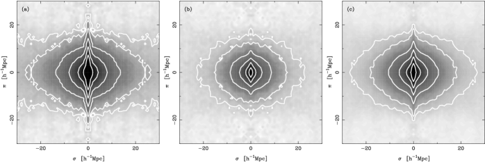
Figure 1: The $\xi(\sigma,\pi)$ grids for our different spectral types: (a) passive, (b) active and (c) full samples. The contour levels are at $\xi$ = 4.0, 2.0, 1.0, 0.5, 0.2 and 0.1.

The correlation function, $\xi$, is measured by comparing the actual galaxy distribution with a catalogue of randomly distributed galaxies. These randomly distributed galaxies are subject to the same redshift and mask constraints as the real data. $\xi(\sigma,\pi)$ is estimated by counting the pairs of galaxies in bins of separation along the line-of-sight, $\pi$, and across the line-of-sight, $\sigma$, using the following estimator,

$$\xi(\sigma,\pi)=\frac{\langle DD\rangle-2\langle DR\rangle-\langle RR\rangle}{\langle RR\rangle}\;,$$ (2)

from Landy & Szalay (1993). In this equation $\langle DD\rangle$ is the weighted number of galaxy-galaxy pairs with particular ($\sigma$,$\pi$) separation, $\langle RR\rangle$ the number of random-random pairs and $\langle DR\rangle$ the number of data-random pairs. The normalisation adopted is that the sum of weights for the real galaxy catalogue should match that of the random catalogue as a function of scale. As in Hawkins et al. (2003) we adopt the $J_{3}$ weighting scheme to minimise the variance in the estimated correlation function (Peebles 1980). We have also estimated the correlation functions using the estimator of Hamilton (1993), however because these give an essentially identical estimate for $\xi$ (well within the statistical uncertainties) we only present the results from the Landy & Szalay estimator in this paper.

The random catalogue is constructed by generating random positions on the sky and modulating the surface density of these points by the completeness variations of the 2dFGRS. Note that, in contrast to Hawkins et al. (2003), this completeness now also includes the that introduced by the spectral classification for galaxies with $z<0.15$ (Norberg 2001). The redshift distribution is then drawn from the selection function of each type as calculated from the 2dFGRS luminosity functions – which allow us to naturally incorporate the varying magnitude limit of the survey. These luminosity functions have been calculated as in Madgwick et al. (2002a) for the data used in this analysis in both the NGP and SGP regions separately for each spectral type.

Due to the design of the 2dF instrument, fibres cannot be placed closer than approximately 30 arcsec (Lewis et al. 2002). In Hawkins et al. (2003) the effects of these so-called ‘fibre collisions’ were taken into account in the estimation of the correlation functions by comparing the angular correlation functions of the parent and redshift catalogues. It was found that the effect was significant for separations $<0.2\,h^{-1}\,{\rm Mpc}$. This cannot be done for the present analysis because of the spectral type selection and so we ignore all separations $<0.2\,h^{-1}\,{\rm Mpc}$ in the fitting process.

The resulting estimates of $\xi(\sigma,\pi)$ are presented in Fig. 1 and clear differences are immediately visible. The rest of this paper is spent quantifying these differences.

3.1 De-correlating error bars

Many of the subsequent sections of this paper will involve attempting to fit a parametric form to $\xi(\sigma,\pi)$ or $\xi(r)$. Because the individual points we estimate for each of these quantities and their associated error bars are not independent (a single galaxy can contribute to correlations over all scales), a simple $\chi^{2}$ fit between the observed and model correlation functions may not yield the most accurate parameter fit. For this reason we must carefully account for these correlations in each of our subsequent fits.

When fitting the model correlation function to the observed $\xi$, we are interested in minimising the residual between the two. For this reason we make a simple change of variables to define,

$$\Delta(s_{i})=\frac{(\xi(s_{i})-\langle\xi(s_{i})\rangle)}{\sigma_{\xi}(s_{i})}\;.$$ (3)

Where here $\xi(s)$ is a given realisation of the correlation function we are estimating, $\langle\xi(s_{i})\rangle$ is the mean value of our ensemble of correlation functions at separation $s_{i}$, and $\sigma_{\xi}(s_{i})$ is the standard deviation of the estimates of the correlation function at this same separation, as deduced from the bootstrap analysis described below. We then construct the covariance matrix,

$$C_{ij}=\langle\Delta(s_{i})\Delta(s_{j})\rangle$$ (4)

in terms of these variables.

The best-fitting model correlation function $\xi^{\rm model}({{s}})$ can be found through minimising the residual between it and the observed correlation function $\xi^{\rm obs}({{s}})$ in terms of the $\chi^{2}$ difference between the two. The residual between the models and observations is defined by,

$$\Delta^{\rm(res)}(s_{i})=\frac{\bigl{(}\xi^{\rm obs}(s_{i})-\xi^{\rm model}(s_{i})\bigr{)}}{\sigma_{\xi}(s_{i})}\;,$$ (5)

in which case the $\chi^{2}$ can be found from,

$$\chi^{2}=(\vec{\Delta}^{\rm(res)})^{\rm T}C^{-1}\vec{\Delta}^{\rm(res)}\;.$$ (6)

Where $\vec{\Delta}^{\rm(res)}$ is the vector of elements given in Eqn. 5. The above equations can then easily be generalised for the gridded $\xi(\sigma,\pi)$. Because the points in the $\xi(\sigma,\pi)$ grid are highly correlated there are in fact very few independent components in the observed correlation function. For this reason it is also possible to extend this analysis as demonstrated by Porciani & Giavalisco (2001) by instead first performing a principal component analysis using our estimated covariance matrix, however we have not found this step to be necessary for this analysis.

One would require a set of independent realisations in order to determine unbiased estimates of $\sigma_{\xi}$ and the data covariance matrix $C$. However, this is of course not possible since we have at our disposal only one realisation of the Universe. In most cases a good determination of this covariance can nonetheless be determined from mock galaxy simulations (e.g. Cole et al. 1998). These simulations are very useful in that they represent the total expected cosmic variance.

The complication we encounter as opposed to other analyses (e.g. Hawkins et al. 2003) is that the simulations available to us cannot adequately account for the variation in galaxy clustering for different types of galaxies. For this reason these simulations can only provide us with rough estimates as to the magnitude of the cosmic variance – which we must somehow scale to correspond to our results.

Another method for determining the expected covariance of our data is to use a bootstrap re-sampling of the data-set (Ling, Barrow & Frenk 1986). The most important assumption in a bootstrap estimation of the covariance matrix is that each of the data-points sampled must be independent. This is not true of the galaxy distribution itself, but if we divide our survey area into a selection of contiguous regions and re-sample these in our bootstrap calculations this assumption will hold (so long as each of the sectors of sky is large enough to be representative). For this reason, in our subsequent analysis, we divide the SGP region of the 2dFGRS survey into eight sectors and the NGP into six. The selection of the regions has been made to ensure a statistically significant and roughly equal number of galaxies in each sector. These regions are then selected at random, with replacement, as in the standard bootstrap analysis. We make use of 20 bootstrap realisations in the analyses that follow, and use these to estimate the covariance matrix for each of our fits. The limitation of the bootstrap approach is that the samples are drawn from the observed volume of space, and may not represent the entire cosmic scatter. However, we find that error bars on parameters derived from the mocks using the procedure of Hawkins et al. (2003) are in reasonable agreement with those derived from our bootstrap approach (see Table 2).

3.2 The real-space correlation function

Because the various redshift distortions to the correlation function only affect its measurement along the line-of-sight, it is possible to make an estimate of the real-space correlation function $\xi(r)$ by first projecting the two-dimensional correlation function, $\xi(\sigma,\pi)$, onto the $\pi=0$ axis. This projected correlation function, $\Xi(\sigma)$, is given by,

$$\Xi(\sigma)=2\int_{0}^{\infty}\xi(\sigma,\pi)d\pi\;.$$ (7)

In practice the upper limit of the integration is taken to be a large finite separation for which the integral is found to converge. We find that limiting the integration to $\pi=70$ $h^{-1}$Mpc suffices for the analysis presented here, providing us with stable projections out to $\sigma=30\;h^{-1}$ Mpc.

The projected correlation function can then be written as an integral over the real-space correlation function (Davis & Peebles 1983),

$$\frac{\Xi(\sigma)}{\sigma}=\frac{2}{\sigma}\int_{\sigma}^{\infty}\frac{r\xi(r)dr}{(r^{2}-\sigma^{2})^{1/2}}\;.$$ (8)

If we assume a power law form; $\xi(r)=(r/r_{0})^{-\gamma}$, we can solve this equation for the unknown parameters,

$$\frac{\Xi(\sigma)}{\sigma}=\left(\frac{r_{0}}{\sigma}\right)^{\gamma}\frac{\Gamma(\frac{1}{2})\Gamma(\frac{\gamma-1}{2})}{\Gamma(\frac{\gamma}{2})}\;.$$ (9)

The projected correlation functions, $\Xi(\sigma)/\sigma$, are shown in Fig. 2, together with error bars derived from the bootstrap realisations. It can be seen that for both sets of galaxies the power law assumption we have made is justified on small scales, and is quite consistent with the observations on large scales. The results from fitting a power law form for $\xi(r)$ are given in Table 1 (Method $P$), together with those derived for the combined sample of all spectrally typed galaxies. Upon comparing with Hawkins et al. (2003), we find that our estimate of the combined correlation function is essentially identical – from which we can conclude that restricting our analysis to only those galaxies with spectral types has not biased our results in any noticeable way.

In order to independently verify our assumption of a power law $\xi(r)$, we have also calculated the real space correlation function, using the non-parametric method of Saunders, Rowan-Robinson & Lawrence (1992) (Fig. 3). It can be seen that this method also estimates a power-law form for $\xi(r)$ out to scales of $\sim 20\;h^{-1}$ Mpc and the best-fit parameters are shown in Table 1 (Method $I$). We note however that a clear shoulder appears to be present in both the correlation functions for separations $r\sim 8\,h^{-1}\,{\rm Mpc}$. It has recently been suggested that this may reflect the transition scale between a regime dominated by galaxy pairs in the same halo and a regime dominated by pairs in separate halos (e.g. Zehavi et al. 2003; Magliochetti & Porciani 2003).

To increase the accuracy of our results we have split the galaxy sample into only two sub-samples. To justify this choice we have repeated our analysis on two further sub-samples of the active sample. We found that the $\xi(r)$ estimates were essentially identical (and consistent within the estimated uncertainties), and so the clustering statistics are relatively insensitive to the exact amount of star-formation occurring in active star-forming galaxies.

Figure 2: The projected correlation function, $\Xi(\sigma)/\sigma$, is shown for both relatively passive and active galaxies in the 2dFGRS. It can be seen that the correlation function of both sets of galaxies has an approximate power law form for a large range of separations, and this is illustrated with the best-fitting power law determined from this data (solid line). The dashed lines are extrapolations of these fits to larger and smaller scales.

Figure 3: The non-parametric estimates of the real-space correlation functions are shown for both our spectral types, using the method of Saunders, Rowan-Robinson & Lawrence (1992). It can be seen that our assumption of a power law form for $\xi(r)$ is justified out to scales of up to $20\;h^{-1}$ Mpc. The solid lines are the best-fitting power law fits shown in Table 1, whereas the dashed lines are extrapolations of these fits.

Table 1: The derived parameters of the projected real-space correlation function. The fits have been determined using the range of separations $0.2<r<20\;h^{-1}$Mpc. The Method column refers to the projected ($P$) or inverted ($I$) values of the parameters. Also shown are the values of $\sigma_{8}^{\scriptscriptstyle\rm NL}$ derived from these correlation functions. Note that the lower limit of the fits ($0.2\;h^{-1}$ Mpc) was imposed to avoid biases from fibre collisions (see Hawkins et al. 2003).

Galaxy type	Method	$r_{0}$ ($h^{-1}$Mpc)	$\gamma$	$\sigma_{8}^{\scriptscriptstyle\rm NL}$
All	$P$	$4.69\pm 0.22$	$1.73\pm 0.03$	$0.83\pm 0.06$
Passive	$P$	$6.10\pm 0.34$	$1.95\pm 0.03$	$1.12\pm 0.10$
Active	$P$	$3.67\pm 0.30$	$1.60\pm 0.04$	$0.68\pm 0.10$
All	$I$	$5.01\pm 0.23$	$1.64\pm 0.03$	$0.88\pm 0.05$
Passive	$I$	$5.97\pm 0.29$	$1.93\pm 0.03$	$1.09\pm 0.08$
Active	$I$	$4.12\pm 0.32$	$1.50\pm 0.04$	$0.75\pm 0.09$

3.3 Relative bias

The term bias is used to describe the fact that it is possible for the distribution of galaxies to not trace the underlying mass density distribution precisely. The existence of such an effect would be a natural consequence if galaxy formation was enhanced, for example, in dense environments. The simplest model commonly assumed (somewhat ad-hoc) to quantify the degree of biasing present, is that of the linear bias parameter, $b$,

$$\left(\frac{\delta\rho}{\rho}\right)_{\rm galaxies}=b\left(\frac{\delta\rho}{\rho}\right)_{\rm mass}\;,$$ (10)

where $\rho$ is a measure of the density, of either the mass or the galaxies. A more specific model, based on the statistics of peaks (Kaiser 1984; Bardeen et al. 1986), is that the degree of clustering we observe in our galaxy sample, quantified in terms of the correlation function, $\xi(r)$, is related to the mass correlation function in terms of,

$$\xi(r)_{\rm galaxies}=b^{2}\xi(r)_{\rm mass}\;.$$ (11)

Where here $b$ is a constant that does not vary with scale, but more generally may depend on $r$.

It is possible to estimate the magnitude of the biasing present in a sample of galaxies through the use of ‘redshift-space distortions’, and this issue will be addressed later in this paper. However, before proceeding it is already possible for us to determine the degree of relative biasing between our galaxy types at different scales, since,

$$\frac{b^{2}_{\rm passive}(r)}{b^{2}_{\rm active}(r)}\equiv\frac{\xi_{\rm passive}(r)}{\xi_{\rm active}(r)}\;.$$ (12)

This relative bias between our two samples is shown in Fig. 4, where we have taken the ratio between the two estimates of the real-space correlation function, derived in the previous section. It can be seen that on small scales the clustering of the most passive galaxies in our sample is significantly larger than that of the more actively star-forming galaxies. The relative bias then appears to decrease significantly until on scales greater than about $\sim 10\;h^{-1}$ Mpc both samples display essentially the same degree of clustering (within the stated uncertainties).

Figure 4: The relative bias between the most passive and actively star-forming galaxies is shown, in terms of (the square-root of) the ratio of the real-space correlation functions of these two samples.

Another frequently used method of quantifying the degree of biasing present in a galaxy sample is through the parameter $\sigma_{8}^{\scriptscriptstyle\rm NL}$ – the dimensionless standard deviation of (in this case) counts of galaxies in spheres of $8\;h^{-1}$ Mpc radius. This quantity was deemed particularly useful because of the recognition (Peebles 1980) that for optically selected galaxies $\sigma_{8}^{\scriptscriptstyle\rm NL}\sim 1$, making the interpretation of $b$ particularly simple since,

$$b=\frac{\sigma_{8}^{\scriptscriptstyle\rm NL}(\rm galaxies)}{\sigma_{8}^{\scriptscriptstyle\rm NL}(\rm mass)}\;.$$ (13)

Note that we write explicitly $\sigma_{8}^{\scriptscriptstyle\rm NL}$ to emphasise that this is a quantity defined on the nonlinear density field. It is an unfortunate standard convention that, in the context of CDM models, $\sigma_{8}$ is used to denote an amplitude calculated according to linear theory. This is not the quantity considered here.

With $b$ defined in this way, the relative bias between our two spectral types is,

$$\frac{b_{\rm passive}}{b_{\rm active}}=\frac{\sigma_{8}^{\scriptscriptstyle\rm NL}(\rm passive)}{\sigma_{8}^{\scriptscriptstyle\rm NL}(\rm active)}\;.$$ (14)

The quantity $\sigma_{8}^{\scriptscriptstyle\rm NL}$ can be directly derived from our measured correlation functions in quite a straight-forward manner, since the expected variance of the galaxy counts in a randomly placed sphere is,

$$\langle(N-\bar{N})^{2}\rangle_{R}=\bar{N}+\left(\frac{\bar{N}}{V}\right)^{2}\int_{R}dV_{1}dV_{2}\xi({\bf{r}})\;.$$ (15)

The first term is the shot-noise contribution and depends on how sparsely we have sampled the galaxy distribution. If we assume a power law form for the real-space correlation function we can estimate the fluctuation amplitude with the shot noise removed as,

$$(\sigma_{8}^{\scriptscriptstyle\rm NL})^{2}\equiv J_{2}(\gamma)\left(\frac{r_{0}}{8}\right)^{\gamma}\;,$$ (16)

where,

$$J_{2}(\gamma)=\frac{72}{[(3-\gamma)(4-\gamma)(6-\gamma)2^{\gamma}]}\;,$$ (17)

(Peebles 1980).

Our derived values of $\sigma_{8}^{\scriptscriptstyle\rm NL}$, for each of the galaxy samples considered in the previous Section, are given in Table 1. It can be seen from this table that the relative bias of passive with respect to active galaxies (integrated over scales up to $8\;h^{-1}$ Mpc) is $b_{\rm passive}/b_{\rm active}=1.09/0.75=1.45\pm 0.14$.

3.4 Modelling $\xi(\sigma,\pi)$

There is much further information to be derived from the observed $\xi(\sigma,\pi)$ grids (Fig. 1) for each galaxy type. However, in order to do so we must first assume some model for the clustering of galaxies with which to contrast the observations. Here we follow the analysis presented in Hawkins et al. (2003) with only minor modifications. Because the most significant limitation to this analysis is inevitably the assumptions that must be enforced upon our model, we summarise here the most important aspects of this model.

In order to derive a model to fit the observed $\xi(\sigma,\pi)$ grid, we need three main ingredients. The first is to assume some form for the real-space correlation function $\xi(r)$. Because we are only going to be concerned with relatively small-scale separations between galaxies ($\leq 20\;h^{-1}$Mpc), we shall assume a power-law form of this function,

$$\xi(r)=\left(\frac{r}{r_{0}}\right)^{-\gamma}\;.$$ (18)

In converting from real space to redshift space the next step is to account for the distortions in the correlation function which are caused by the linear coherent in-fall of galaxies into cluster over-densities (Kaiser 1987; Hamilton 1992), combined with non-linear velocity dispersion (e.g. Peacock et al. 2001). The linear-theory in-fall distortion can be written as (Hamilton 1992):

$$\xi^{\prime}(\sigma,\pi)=\xi_{0}(s)P_{0}(\mu)+\xi_{2}(s)P_{2}(\mu)+\xi_{4}(s)P_{4}(\mu)\;,$$ (19)

where P${}_{\ell}(\mu)$ are Legendre polynomials, $\mu=\cos(\theta)$ and $\theta$ is the angle between $r$ and $\pi$. The relations between $\xi_{\ell}$, $\xi(r)$ and $\beta$ for a simple power-law $\xi(r)=(r/r_{0})^{-\gamma}$ are

$$\xi_{0}(s)=\left(1+\frac{2\beta}{3}+\frac{\beta^{2}}{5}\right)\xi(r)\;,$$ (20)

$$\xi_{2}(s)=\left(\frac{4\beta}{3}+\frac{4\beta^{2}}{7}\right)\left(\frac{\gamma}{\gamma-3}\right)\xi(r)\;,$$ (21)

$$\xi_{4}(s)=\frac{8\beta^{2}}{35}\left(\frac{\gamma(2+\gamma)}{(3-\gamma)(5-\gamma)}\right)\xi(r).$$ (22)

We use these relations to create a model $\xi^{\prime}(\sigma,\pi)$ which we then convolve with the distribution function of random pairwise motions, $f(v)$, to give the final model (Peebles 1980):

$$\xi(\sigma,\pi)=\int^{\infty}_{-\infty}\xi^{\prime}(\sigma,\pi-v/H_{0})f(v)dv$$ (23)

and we choose to represent the random motions by an exponential form,

$$f(v)=\frac{1}{a\sqrt{2}}\exp\left(-\frac{\sqrt{2}|v|}{a}\right)$$ (24)

where $a$ is the pairwise peculiar velocity dispersion (often known as $\sigma_{12}$). An exponential form for the random motions has been found to fit the observed data better than other functional forms (e.g. Ratcliffe et al. 1998; Landy 2002).

The factor $\beta\equiv\Omega_{\rm m}^{0.6}/b$ arises from the growth rate in linear theory,

$$f\equiv\frac{d\ln\delta}{d\ln a}\approx\Omega_{\rm m}^{0.6}\;,$$ (25)

which is almost independent of the cosmological constant (Lahav et al. 1991), combined with the scale-independent biasing parameter $b$. A simple consequence of this model is that the redshift-space power spectrum will also appear to be amplified compared to its real-space counterpart. It is worth explicitly re-stating that all of these derivations are based upon the assumptions of the linear theory of perturbations and linear bias, and assume the far-field approximation (although this is not a significant issue for the 2dFGRS, for which $z_{\rm median}=0.1$).

It is also interesting to note that there is another cosmological effect that can result in the flattening of the observed $\xi(\sigma,\pi)$ contours. It was first noted by Alcock & Paczynski (1979) that the presence of a significant cosmological constant, $\Lambda$, would result in geometric distortions of the inferred clustering if an incorrect geometry was assumed. However, Ballinger, Peacock & Heavens (1996) have shown that this is likely to be negligible for the low redshift data-set being considered here, for our assumed model of $\Omega_{\rm m}=1-\Omega_{\Lambda}=0.3$.

To summarise, the parameters of our model are therefore the real-space correlation function, $\xi(r)=(r/r_{0})^{-\gamma}$, $\beta$, and $f(v)$, parameterised in terms of the velocity dispersion $a$. The best-fitting parameters of this model can now be determined from the model correlation function that best matches the observed $\xi(\sigma,\pi)$.

4 Results

Table 2: The best fitting model parameters derived from the observed $\xi(\sigma,\pi)$ grid are shown. All fits have been made over the quasi-linear redshift-space separation range $8<s<20\;h^{-1}$ Mpc. The quoted uncertainties correspond to the $1\sigma$ scatter derived from the bootstrap estimates (see Fig. 6). For comparison, uncertainties in $\beta$ have also been estimated from sparsely sampled 2dFGRS mock galaxy catalogues (Cole et al., 1998) limited to $z<0.15$, and correspond to $\Delta\beta=0.12$ for the full sample and $\Delta\beta=0.16$ for a 1-in-2 random sampling. This demonstrates that the bootstrap approach has given a fair assessment of the cosmic scatter in these estimates.

Parameter	All galaxies	Passive galaxies	Active galaxies
$\beta$	$0.46\pm 0.10$	$0.48\pm 0.14$	$0.49\pm 0.13$
$a$	$537\pm 87$ km s-1	$612\pm 92$ km s-1	$416\pm 76$ km s-1
$r_{0}$	$5.47\pm 0.32$ $h^{-1}$ Mpc	$7.21\pm 0.34$ $h^{-1}$ Mpc	$4.24\pm 0.41$ $h^{-1}$ Mpc
$\gamma$	$1.75\pm 0.08$	$1.91\pm 0.10$	$1.60\pm 0.11$

4.1 Validation of assumptions

We have calculated the real-space correlation function, $\xi(r)$, independently using the non-parametric method of Saunders, Rowan-Robinson & Lawrence (1992), in order to confirm the range over which it is a power-law (see Fig. 3). For both samples of galaxies, $\xi(r)$ is adequately fit by a power-law to separations of $r<20$ $h^{-1}$ Mpc. This limit provides the upper bound to which we can compare the observed $\xi(\sigma,\pi)$ with our assumed model. In addition, because we have assumed the linear theory of perturbations in deriving our model we must impose a lower limit to the separations that we will use in our fit. To ensure that we have a sufficiently large fitting range we set this lower-limit to $s=8\;h^{-1}$ Mpc. In fact it is quite plausible that the assumptions of linear theory are no longer valid at this separation. However, as will be shown, the ability of our model to recover the observed $\xi(\sigma,\pi)$ at these scales is reassuring.

On large scales it is known that the correlation function must deviate from a pure power law form, and there is some evidence to support this in Section 3.2, on scales $\sim 20\;h^{-1}$ Mpc. A number of methods to account for this expected curvature in $\xi(r)$ were investigated in Hawkins et al. (2003). However, the analysis presented there suggests that so long as we restrict our fitting range to $r<20\;h^{-1}$ Mpc the curvature has a negligible impact upon our parameter estimation. For this reason we neglect the possibility of curvature in the present analysis and restrict ourselves to using the simple power-law form for $\xi(r)$.

The other major assumption we have made is that the peculiar velocity distribution, $f(v)$, has an exponential form. This can be tested using the method outlined by Landy, Szalay & Broadhurst (1998). This method makes a non-parametric estimate of the velocity distribution, using the Fourier decompositions of the observed $\xi(\sigma,\pi)$ grid along the $k_{\sigma}=0$ and $k_{\pi}=0$ axes. Unfortunately this method ignores the effects of coherent in-fall, which can substantially change the resulting estimate of $a$ (see Hawkins et al. 2003). However, it is found that the recovered $f(v)$ is well fit by an exponential form – for both types of galaxies. Hawkins et al. (2003) have shown that although incorporating the effects of coherent in-fall changes the estimated velocity dispersion, $a$, substantially, the method gives a robust estimate of the form for $f(v)$.

4.2 Parameter fits

All four of our parameters ($\beta$, $a$, $r_{0}$ and $\gamma$) are allowed to vary over a large range of possibilities and a downhill simplex multi-dimensional minimisation routine is adopted to find their best-fitting values (see e.g. Press et al. 1992). Our calculated $\xi(\sigma,\pi)$ contours are shown in Fig. 5, together with those of the best-fitting model correlation functions derived in this manner. The peak parameters of this best-fitting model are detailed in Table. 2 together with their estimated uncertainties. We find that there is quite a significant degeneracy between $\beta$ and $a$ (see Fig. 6). This is also exacerbated by the relatively noisy nature of $\xi(r)$ at these scales, which makes $r_{0}$ and $\gamma$ difficult to constrain accurately.

One immediate conclusion is that the velocity dispersions of the two galaxy populations are very distinct, even taking into account the substantial statistical uncertainties. This is an interesting result which has significant implications for the proportion of each of these galaxy types we expect to occupy large, virialised clusters of galaxies.

Another conclusion that we can easily make is to quantify the relative bias between our two spectral types, as described in Section 3.3. However, as demonstrated in that Section, the relative bias between our galaxy types is in fact essentially unity over the range for which our model assumptions are valid ($8-20\;h^{-1}$ Mpc), a result confirmed in this analysis. However, a much more important quantity that can be inferred from these redshift-space distortions, that could not be determined previously, is the absolute value of the biasing between the galaxy and mass distributions, $b$, as described in Section 3.3. We return to this point in the next Section of this paper.

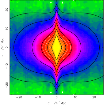
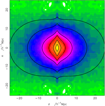
Figure 5: The full $\xi(\sigma,\pi)$ grids for our different spectral types: passive (left) and active (right). Also plotted (white lines) are the contour levels of the best-fitting model derived earlier. The contour levels are $\xi$ = 4.0, 2.0, 1.0, 0.5, 0.2, 0.1.

Figure 6: The estimates of $\beta$ and $a$ for the bootstrap samples are shown for both the passive (squares) and active (triangles) galaxy samples. It can be seen that a significant degeneracy exists between $\beta$ and $a$, for both samples. The fits have been made using only the quasi-linear regime of $8-20\;h^{-1}$Mpc. The crosses show the fits to the full samples together with the $1\sigma$ uncertainties shown in Table 2.

5 Comparison with Previous Results

Table 3: Comparison between biasing results derived using the 2dF Galaxy Redshift Survey by various authors. The results of Peacock et al. (2001) are derived from the redshift-space distortions in the two-point correlation function (Note that this galaxy sample was much deeper as galaxies without spectral types were used). Lahav et al. (2002) made their estimate of the bias through comparing the amplitude of fluctuations in both the 2dFGRS and the CMB. Verde et al. (2002) calculated the bi-spectrum of the 2dFGRS, which constrained the linear bias parameter, $b$, which we have converted to $\beta$ by assuming our concordance cosmological model of a flat Universe with $\Omega_{\rm m}=0.3$. Note that the results of Lahav et al. (2002) and Verde et al. (2002) are valid over scales expressed in terms of wavenumber $k$ rather than real-space distance. We have converted between the two by simply taking $r\sim 1/k$.

Galaxy type	Author	Scales ($h^{-1}$Mpc)	($z_{\rm s}$, $L_{\rm s}/L_{*}$)	$\beta(z_{\rm s},L_{\rm s})$	$\beta(0,L_{*})$
All	–	$8-20$	(0.11,1.06)	$0.46\pm 0.10$	$0.44\pm 0.09$
Passive	–	$8-20$	(0.11,1.26)	$0.48\pm 0.14$	$0.47\pm 0.14$
Active	–	$8-20$	(0.11,0.95)	$0.49\pm 0.13$	$0.48\pm 0.13$
All	Hawkins et al.	$8-20$	(0.15,1.4)	$0.49\pm 0.09$	$0.47\pm 0.08$
All	Peacock et al.	$8-25$	(0.17,1.9)	$0.43\pm 0.07$	$0.45\pm 0.07$
All	Lahav et al.	$7-50$	(0.17,1.9)	$0.48\pm 0.06$	$0.50\pm 0.06$
All	Verde et al.	$2-10$	(0.17,1.9)	$0.56\pm 0.06$	$0.59\pm 0.06$

Because previous estimates of $\beta$ have used slightly different galaxy samples, it is first necessary to correct for various effects before making a proper comparison (see Lahav et al. 2002). There are two main issues which affect the different estimates of the biasing; the effective redshift of the survey sample used, $z_{\rm s}$, and the effective luminosity of the galaxies in that sample, $L_{\rm s}$. These quantities vary between the samples used, depending on the weighting scheme adopted and the limiting redshift of the survey.

Because we have only used 2dFGRS galaxies for which a spectral type is available our sample is limited to $z_{\rm max}=0.15$. To determine the effective redshift of our sample it is necessary for us to determine the weighted average of the galaxies used in each of our calculations. Doing so reveals that for all three of our samples $z_{\rm s}=0.11$. In a similar way we can calculate the weighted mean luminosity of each of our samples, which are found to be as follows. Combined: $L_{\rm s}=1.06L_{*}$; Passive: $L_{\rm s}=1.26L_{*}$; Active: $L_{\rm s}=0.95L_{*}$; where we have taken $M^{*}-5\log_{10}(h)=-19.66$ (Norberg et al. 2002b).

Assuming linear dynamics and linear biasing, the redshift-distortion parameter, $\beta$, for a given sample redshift and luminosity can be written as,

$$\beta(L,z)\approx\frac{\Omega_{\rm m}^{0.6}(z)}{b(L,z)}\;.$$ (26)

The evolution of the matter density parameter, $\Omega_{\rm m}(z)$ is straight-forward to determine, assuming a given cosmological model,

$$\Omega_{\rm m}(z)=\Omega_{\rm m}(1+z)^{3}(H/H_{0})^{-2}\;,$$ (27)

where $\Omega_{\rm m}$ is the matter density at the present epoch and,

$$\left(\frac{H}{H_{0}}\right)^{2}=\Omega_{\rm m}(1+z)^{3}+(1-\Omega_{\rm m}-\Omega_{\Lambda})(1+z)^{2}+\Omega_{\Lambda}\;.$$ (28)

The determination of the variation in the biasing parameter, $b$, with redshift is much less straight-forward. As shown in Section 3.3, $b$ can be defined as,

$$b(z)=\frac{\sigma_{8}^{\scriptscriptstyle\rm NL}{}^{,\,\rm g}(z)}{\sigma_{8}^{\scriptscriptstyle\rm NL}{}^{,\,\rm m}(z)}\;,$$ (29)

where here we have added a redshift dependence, $b(z)$, and labelled the two $\sigma_{8}^{\scriptscriptstyle\rm NL}$’s by the superscripts $\rm g$ and $\rm m$ to denote galaxies and mass respectively. As described by Lahav et al. (2002), there is now much evidence to suggest that whilst the matter fluctuations continue to grow at low redshifts, the fluctuations in the galaxy distribution are relatively constant between $0<z<0.5$ (see e.g. Shepherd et al. 2001). If we assume that the matter fluctuations grow according to the linear theory of perturbations then, $\sigma_{8}^{\scriptscriptstyle\rm NL}{}^{,\,\rm m}(z)=\sigma_{8}^{\scriptscriptstyle\rm NL}{}^{,\,\rm m}(0)D(z)$, where $D(z)$ is the growing mode of fluctuations (Peebles 1980). Whereas, $\sigma_{8}^{\scriptscriptstyle\rm NL}{}^{,\,\rm g}(L,z)\approx\sigma_{8}^{\scriptscriptstyle\rm NL}{}^{,\,\rm g}(L,0)$. Therefore,

$$b(L,z)=\frac{b(L,0)}{D(z)}$$ (30)

The final step then is to correct the biasing parameter, $b$, for the luminosity of our sample. Norberg et al. (2001) found from the analysis of the galaxy correlation functions on scales $<10\;h^{-1}$ Mpc that,

$$\frac{b(L,0)}{b(L_{*},0)}=0.85+0.15\left(\frac{L}{L_{*}}\right)\;.$$ (31)

Assuming that this relation also holds in our quasi-linear regime of $8-20\;h^{-1}$ Mpc, then allows us to determine $\beta$ at redshift $z=0$ and luminosity $L=L_{*}$.

Table 3 shows the results for $\beta$ derived in the analysis presented here, both before and after converting to redshift $z=0$ and luminosity $L=L_{*}$. Also shown are other results derived from the 2dFGRS by previous authors. It can be seen that there is a remarkably good agreement between all the results presented. We note that these results have been derived by applying linear corrections to a selection of quasi-linear regimes, which may introduce systematic errors into our results. This is a particular concern for the results of Verde et al. (2002), which correspond to the smallest separation ranges used.

6 Discussion

We have derived a variety of different parameterisations for the 2dFGRS correlation function, $\xi(\sigma,\pi)$, for different spectral types. The two types we have used can roughly be interpreted as dividing our galaxy sample on the basis of their relative amount of current star-formation activity, and hence provide useful insight into how galaxy formation may relate to the large-scale structure of the galaxy distribution. The actual cut we have imposed is most naturally interpreted in terms of the Scalo birthrate parameter, $b_{\rm Scalo}$. This is defined to be the ratio of the current star-formation rate and the past averaged star-formation rate. Adopting this convention, our cut of $\eta=-1.4$ corresponds to dividing our sample into galaxies with $b_{\rm Scalo}=0.1$, i.e. between galaxies whose present star formation rate is greater or less than 10% of their past averaged rate.

6.1 Relative bias on small scales

On scales smaller than $\sim 8\;h^{-1}$ Mpc the clustering of passive galaxies is much stronger than that of the more actively star-forming galaxies. This was demonstrated quantitatively by the real-space correlation functions derived in Section 3.2, for which the passive galaxy sample were fit by a power-law with larger scale length, $r_{0}$ and steeper $\gamma$. In addition it was shown that the values of $\sigma_{8}^{\scriptscriptstyle\rm NL}$ derived for each of these samples were quite distinct, being $\sigma_{8}^{\scriptscriptstyle\rm NL}=1.09\pm 0.08$ for the passive galaxies and $\sigma_{8}^{\scriptscriptstyle\rm NL}=0.75\pm 0.09$ for the actively star-forming galaxies, implying an (integrated) relative bias between our two types of,

$$\frac{b_{\rm passive}}{b_{\rm active}}=1.45\pm 0.14\;,$$ (32)

at the effective redshift and luminosity of our galaxy samples (see Table 3). Note that this ratio quantifies the integrated relative bias between scales of $0-8\;h^{-1}$ Mpc.

Our correlation functions per type confirm that the slope of passive (early type) galaxies is steeper than that of active (late tape) galaxies (cf. Zehavi et al. 2001). On the other hand, the slope of the correlation functions derived for different luminosity ranges show no significant variation (Norberg et al. 2001, 2002a; Zehavi et al. 2001). These results call for theoretical explanations and they set important constraints on models for galaxy formation.

6.2 Velocity dispersions

The velocity distributions of our two samples were found to be distinct. The passive galaxy sample displayed a consistently larger velocity dispersion, $a$, than the actively star-forming sample on all scales, and in particular on separations of $8-20\;h^{-1}$ Mpc were found to be $612\pm 92$ and $416\pm 76$ km s^-1 respectively. This result is consistent with the observations of Dressler (1980), that a significant morphology-density relation exists – since a larger velocity dispersion would tend to suggest a higher proportion of galaxies occupying virialised (high-density) clusters.

6.3 Relative bias on large scales

The determination of the redshift-distortion parameter, $\beta$, was found to be much less straight-forward. The evidence from our analysis is that $\beta$ has only a relatively small dependence on the spectral type of the galaxy sample under investigation. We found that on scales of $8-20\;h^{-1}$ Mpc, the two redshift distortion parameters were; $\beta=0.48\pm 0.14$ and $\beta=0.49\pm 0.13$ for the passive and actively star-forming galaxy samples respectively, yielding a relative bias of only,

$$\frac{b_{\rm passive}}{b_{\rm active}}=1.02\pm 0.40.$$ (33)

The overall redshift-distortion parameter, $\beta$, independent of spectral type is found here to be $0.46\pm 0.10$ (on scales of $8-20\;h^{-1}$ Mpc), at our sample’s mean redshift and luminosity. By making various assumptions (Section 5) this result can be converted to redshift $z=0$ and $L_{*}$ luminosity, giving $\beta(0)=0.44\pm 0.09$. This result is is almost identical to the $\beta(0)=0.47\pm 0.08$ derived from the results of Hawkins et al. (2003), using the entire 2dFGRS data-set, over the same separation range.

In the analyses presented in this paper two fundamental limits were found to greatly inhibit our ability to accurately characterise the relative and absolute biases on different scales. The first of these was that on small scales – where the clustering of our two populations is most distinct – the assumptions of our model of the galaxy clustering were no longer accurate, and so we could not accurately determine $\beta$ or $a$ on these scales. Our second limitation was found on large scales ($s\sim 20\,h^{-1}\,{\rm Mpc}$), where the galaxy correlation functions became noisy and were no longer well parameterised by a power-law form.

The latter of these issues can be addressed to some degree simply by a change of formalism to incorporate the power spectrum estimations of each galaxy type or colour (Peacock 2003). Because this characterisation of the clustering is more sensitive to larger scales of separations it would allow us to more rigorously test whether the large-scale ($s>20\,h^{-1}\,{\rm Mpc}$) clustering of these populations are in fact distinct and also allow us to incorporate the possibility of scale-dependent bias. The derived correlation functions per type could also be used within the framework of halo occupation number to derive e.g. the mean number of galaxies of a given type per halo (e.g. Zehavi et al. 2003; Magliochetti & Porciani 2003).

References

- [1] Alcock C., Paczynski B., 1979, Nature, 281, 358
- [2] Ballinger W. E., Peacock J. A., Heavens A. F., 1996, MNRAS, 282, 877
- [3] Bardeen J. M., Bond J. R., Kaiser N., Szalay A. S., 1986, ApJ, 304, 15
- [4] Cole S., Hatton S., Weinberg D.H., Frenk C.S., 1998, MNRAS, 300, 945
- [5] Colless M. M., et al. (the 2dFGRS Team), 2001, MNRAS, 328, 1039
- [6] Davis M., Geller M. J., 1976, ApJ, 208, 13
- [7] Davis M., Peebles P. J. E., 1983, ApJ, 267, 465
- [8] Dekel A., Lahav O., 1999, ApJ, 520, 24
- [9] Dressler A., 1980, ApJ, 236, 351
- [10] Hamilton A. J. S., 1992, ApJ, 385, L5
- [11] Hamilton A. J. S., 1993, ApJ, 417, 19
- [12] Hawkins E., et al. (the 2dFGRS Team), 2003, MNRAS submitted (astro-ph/0212375)
- [13] Hermit S., Santiago B. X., Lahav O., Strauss M. A., Davis M., Dressler A., Huchra J. P. 1996, MNRAS, 283, 709
- [14] Kaiser N., 1984, ApJ, 284, 9
- [15] Kaiser N., 1987, MNRAS, 227, 1
- [16] Kennicutt R. C., Jr., 1992, ApJS, 79, 255
- [17] Lahav O., Nemiroff R. J., Piran T., 1990, ApJ, 350, 119
- [18] Lahav O., Rees M. J., Lilje P. B., Primack J. R., 1991, MNRAS, 251, 128
- [19] Lahav O., et al. (the 2dFGRS Team), 2002, MNRAS, 333, 961
- [20] Landy S. D., Szalay A. S., 1993, ApJ, 412, 64
- [21] Landy S. D., Szalay A. S., Broadhurst T. J., 1998, ApJ, 494, 133
- [22] Landy S. D., 2002, ApJ, 567, L1
- [23] Lewis I.J., et al., 2002, MNRAS, 333, 279
- [24] Ling E. N., Barrow J. D., Frenk C. S., 1986, MNRAS, 223, 21
- [25] Loveday J., Tresse L., Maddox S., 1999, MNRAS, 310, 281
- [26] Madgwick D. S., 2002, MNRAS, 338, 197
- [27] Madgwick D. S., et al. (the 2dFGRS Team), 2002a, MNRAS, 333, 133
- [28] Madgwick D., Somerville R., Lahav O., Ellis R., 2002b, MNRAS submitted (astro-ph/0210471)
- [29] Magliochetti M., Porciani C., 2003, in preparation
- [30] Norberg P., 2001, PhD Thesis, University of Durham
- [31] Norberg P., et al. (the 2dFGRS Team), 2001, MNRAS, 328, 64
- [32] Norberg P., et al. (the 2dFGRS Team), 2002a, MNRAS, 332, 827
- [33] Norberg P., et al. (the 2dFGRS Team), 2002b, MNRAS, 336, 907
- [34] Peacock J. A., et al. (the 2dFGRS Team), 2001, Nature, 410, 169
- [35] Peacock J. A., 2003, to appear in ’The Emergence of Cosmic Structure’, Eds. S. Holt & C. Reynolds (AIP), astro-ph/0301042
- [36] Peebles, P. J. E., 1980, ‘The Large Scale Structure of the Universe’, Princeton Univ. Press, Princeton
- [37] Pen U., 1998, ApJ, 504, 601
- [38] Porciani C., Giavalisco M., 2002, ApJ, 565, 24
- [39] Press W. H., Teukolsky S. A., Vetterling W. T., Flannery B. P., 1992, ‘Numerical Recipes’, Cambridge University Press, Cambridge U.K.
- [40] Ratcliffe A., Shanks T., Parker Q. A., Fong R., 1998, MNRAS, 296, 191
- [41] Saunders W., Rowan-Robinson M., Lawrence A., 1992, MNRAS, 258, 134
- [42] Scalo J. M., 1986, Fund. Cos. Phys., 11, 1
- [43] Shepherd C. W., et al. 2001, ApJ, 560, 72
- [44] Tegmark M., Hamilton A. J. S., Yongzhong X., 2001, MNRAS, 335, 887
- [45] Verde L., et al. (the 2dFGRS Team), 2002, MNRAS, 335, 432
- [46] Zehavi I., et al. (the SDSS collaboration), 2001, ApJ, 571, 172
- [47] Zehavi I., et al. (the SDSS collaboration), 2003, ApJ submitted (astro-ph/0301280)