Quantum impurity in an antiferromagnet:
non-linear sigma model theory

Abstract

We present a new formulation of the theory of an arbitrary quantum impurity in an antiferromagnet, using the O(3) non-linear sigma model. We obtain the low temperature expansion for the impurity spin susceptibilities of antiferromagnets with magnetic long-range order in the ground state. We also consider the bulk quantum phase transition in $d=2$ to the gapped paramagnet ($d$ is the spatial dimension): the impurity is described solely by a topological Berry phase term which is an exactly marginal perturbation to the critical theory. The physical properties of the quantum impurity near criticality are obtained by an expansion in $(d-1)$.

I Introduction

Recent papers sbv ; vbs have presented a general field theoretical discussion of the low energy properties of a spin $S$ impurity embedded in an antiferromagnet or a superconductor which is in the vicinity of a bulk spin-ordering quantum transition. These studies were motivated by a variety of recent experiments studying Zn and Ni impurities in the cuprate superconductors and spin-gap compounds. The motivations and prior work have been discussed in some detail in Ref. vbs, (hereafter referred to as I), and so will not be repeated here. Further theoretical sushkov ; stv , numerical troyer ; sandvik ; sandvik2 , and experimental vajk work on these issues has also appeared, and we will discuss some of these results below. There has also been related work on impurity models in systems with fermionic excitations si ; demler .

The purpose of this paper is to provide additional results for the same quantum impurity problem using a different field-theoretic formulation. The results in I were obtained using an expansion in $(3-d)$, where $d$ is the spatial dimensionality. Stimulated mainly by the recent results of Höglund and Sandvik sandvik , we have succeeded in obtaining a formulation which permits an expansion in $\epsilon=d-1$, and this will be described in the present paper. The universal scaling structure we shall describe below in the $(d-1)$ expansion turns out to be identical to that obtained in I using the $(3-d)$ expansion. This is strong evidence that a fixed point with the same scaling properties does indeed describe the physical situation in $d=2$.

Throughout this paper, we will implicitly assume in our discussion that $1<d<3$, unless stated otherwise. The only exception is Appendix C, where we will present results in $d=3$. Also we will set $\epsilon=(d-1)$, whereas in I the same symbol was used for $(3-d)$.

Let us outline the main results of I and those that will be presented here. Consider a simple two-dimensional quantum antiferromagnet which undergoes a quantum transition from a magnet Néel state to a gapped, confining paramagnet with only integer spin excitations e.g. a model of coupled spin ladders ladders . We tune the antiferromagnet across this transition with a generalized coupling $g_{0}$, such that there is Néel order for $g_{0}<g_{c}$, and a gapped paramagnet for $g_{0}>g_{c}$. Insert an arbitrary quantum impurity (e.g. a vacancy) which leads to a net deficit or excess of spin $S$ in its vicinity (after accounting for the sublattice alternation). At a temperature $T$ above the gapped paramagnet phase, with $g_{0}>g_{c}$ and a spin gap $\Delta$, this impurity will contribute an impurity spin susceptibility

$$\chi_{\rm imp}=\frac{S(S+1)}{3T}~{}~{}~{}~{}~{};~{}~{}~{}~{}~{}~{}g_{0}>g_{c}$$ (1)

with exponentially small corrections as $T\rightarrow 0$ (we set $\hbar=k_{B}=1$ and have absorbed factors of the gyromagnetic ratio and the Bohr magneton in the definition of the external magnetic field). We can view (1) as a definition of the value of $S$ (which must be an integer or half-odd-integer) for the quantum impurity. In the magnetically ordered phase with $g_{0}<g_{c}$, there are much stronger corrections to the isolated impurity behavior because of the presence of broken spin rotation symmetry at $T=0$ and gapless excitations in the bulk; in dimensions $d\leq 2$ the symmetry is restored at any $T>0$, and corrections to the impurity susceptibility can be written in the scaling formvbs

$$\chi_{\rm imp}=\frac{1}{T}\Phi\left(\frac{T}{[c^{(d-2)}\rho_{s}]^{1/(d-1)}}\right)~{}~{}~{}~{}~{};~{}~{}~{}~{}~{}g_{0}\leq g_{c}$$ (2)

where $\rho_{s}$ is the spin stiffness of the bulk ordered antiferromagnet in the absence of the impurity, and $c$ is the bulk spin-wave velocity. In the limit $T\rightarrow 0$, it was argued in I that $\Phi(0)=S^{2}/3$ exactly. This prediction has been verified recently in the numerical study by Höglund and Sandvik sandvik . On the basis of the $(3-d)$ expansion, the subleading behavior $\Phi(y\rightarrow 0)=S^{2}/3+\mathcal{C}_{3}y$, with $\mathcal{C}_{3}$ a universal number, was proposed for $d=2$ in I. Höglund and Sandvik sandvik also tested this subleading behavior, and argued that it did not hold—instead they proposed the presence of $\ln(1/T)$ term. We will show here that their proposal is indeed correct, and that precisely in $d=2$, the behavior in the limit $T\ll\rho_{s}$ is

$$\Phi(y\rightarrow 0)=\frac{S^{2}}{3}+\frac{S^{2}}{3\pi}y\ln(1/y)+\widetilde{\mathcal{C}_{3}}y$$

$$-\frac{S^{2}}{6\pi^{2}}y^{2}\ln(1/y)+\widetilde{\mathcal{C}}_{4}y^{2}+\ldots,$$ (3)

with $\widetilde{\mathcal{C}}_{3,4}$ unknown universal constants. The $\ln(1/y)$ dependence is special to $d=2$ and does not appear at any finite order in the $(3-d)$ expansion, and this is the reason it was overlooked in I. Subleading singularities in the small $y$ expansion do appear naturally in the $(d-1)$ expansion presented in this paper. We also note here that (3) was obtained with no assumptions on the value of $S$: the $S$ dependencies in the co-efficients are therefore exact.

The subdominant $\ln(1/T)$ dependence implied by (3) (and the anomalous powers of $y$ in (22)) is a consequence of spin-wave Goldstone fluctuations in $1<d\leq 2$, and does not involve the critical singularities at $g_{0}=g_{c}$ in an essential way. Consequently, in $d=2$, this $\ln(1/T)$ dependence should also be present in antiferromagnets with $g_{0}\ll g_{c}$, which are not especially close to any quantum critical point. In this situation can surmise that (3) implies

$$\chi_{\rm imp} = \frac{S^{2}}{3T}\Biggl{[}1+\frac{T}{\pi\rho_{s}}\ln\left(\frac{C_{1}\rho_{s}}{T}\right)-\frac{T^{2}}{2\pi^{2}\rho_{s}^{2}}\ln\left(\frac{C_{2}\rho_{s}}{T}\right)$$ (4)

$$+ \mathcal{O}\left(\frac{T}{\rho_{s}}\right)^{3}\Biggr{]}~{};~{}g_{0}\ll g_{c}~{},~{}T\rightarrow 0~{},~{}d=2~{}~{}~{}~{}$$

where, in general, the constants $C_{1,2}$ are non-universal; only as we approach the quantum critical point and $\rho_{s}\rightarrow 0$ do $C_{1,2}$ become universal, and then (4) is seen to be consistent with (3). The $\ln(1/T)$ correction in (4) is related to the logarithmic frequency dependencies discussed by Nagaosa et al.nagaosa and Chernyshev et al. castro . To the extent that sharp spin-waves are also present in ordered metallic antiferromagnets, (4) may also apply to such systems morr .

As we will see shortly, (4) is obtained for the case where the coupling between the impurity and the bulk antiferromagnet has scaled to infinity. This implies that at low energies the impurity moment is effectively locked along the direction of the local orientation of the bulk antiferromagnetic order. While such locking is appropriate near the quantum critical point, it is not a priori clear whether it should also hold at low $T$ above a well ordered antiferromagnet with $g_{0}\ll g_{c}$. We will briefly address this issue by also examining the case of finite coupling (see Appendix B): we find that the co-efficient of the $(1/\rho_{s})\ln(1/T)$ term in (4) remains universal, but there are non-universal corrections to the $T\ln(1/T)$ term.

A separate category of our results concern $\chi_{\rm imp}$ at the quantum critical point, $g_{0}=g_{c}$. These correspond to the large $y$, $T\gg\rho_{s}$, limit of (2). Here, it was argued in I that

$$\Phi(y\rightarrow\infty)=\mathcal{C}_{1}$$ (5)

with $\mathcal{C}_{1}$ a universal number. A $(3-d)$ expansion for $\mathcal{C}_{1}$ was provided in I, and it contained non-trivial corrections to the free moment value of $S(S+1)/3$. Sushkov sushkov has questioned the existence of such corrections, but we reply to his arguments in Appendix D. The present paper will show that (5) is obeyed also in the $(d-1)$ expansion: in this case the $(d-1)$ expansion provides terms as corrections to the ‘classical’ moment value of $S^{2}/3$, and details of this appear in the body of the text, and the final result is in (42).

A number of other results for universal properties of the impurity correlations were provided in I using the $(3-d)$ expansion. All of these can also be computed in the $(d-1)$ expansion, and in every case we find complete agreement in the structure of the scaling properties. Details of such computations also appear in the body of this paper.

The following section will introduce the non-linear sigma model field theory which describes the dynamics of an impurity in a quantum antiferromagnet. Section III will then discuss the perturbative structure of this theory, with details of the perturbative computations appearing in Appendix A. We will show how to deduce low temperature properties using this perturbation theory. Finally, Section IV presents a renormalization analysis which allows us to deduce the physical characteristics of the critical point.

II Field Theory

This section will introduce the field-theoretical formulation of the quantum impurity dynamics which enables an expansion of its universal properties in the $(d-1)$ expansion. In contrast to our earlier $(3-d)$ expansion, which used a ‘soft-spin’ formulation of the bulk antiferromagnetic fluctuations, the present $(d-1)$ expansion will use the ‘fixed-length’ representation of the O(3) non-linear sigma model.

We begin by recalling our earlier ‘soft-spin’ formulation. The bulk spin fluctuations of the antiferromagnet are represented by the real field $\phi_{\alpha}(x,\tau)$, with $\alpha=1\ldots 3$ an index representing the spin component, $x$ a $d$-dimensional spatial co-ordinate, and $\tau$ is imaginary time. The impurity spin is placed at the origin of co-ordinates $x=0$, and is represented by a unit length field $n_{\alpha}(\tau)$, and the bulk and impurity fluctuations are coupled in the partition function

$$\widetilde{\mathcal{Z}}=\int\mathcal{D}\phi_{\alpha}(x,\tau)\mathcal{D}n_{\alpha}(\tau)\delta\left(n_{\alpha}^{2}-1\right)$$

$$~{}~{}~{}~{}~{}~{}~{}~{}~{}~{}~{}~{}~{}~{}~{}~{}~{}~{}~{}~{}~{}~{}~{}~{}\exp\left(-\widetilde{\mathcal{S}}_{\text{b}}[\phi_{\alpha}]-\widetilde{\mathcal{S}}_{\text{imp}}\right)$$

$$\widetilde{\mathcal{S}}_{\text{imp}}=\int_{0}^{1/T}d\tau\bigg{[}iSA_{\alpha}(n)\frac{dn_{\alpha}(\tau)}{d\tau}$$

$$~{}~{}~{}~{}~{}~{}~{}~{}~{}~{}~{}~{}~{}~{}~{}~{}~{}~{}~{}~{}~{}~{}~{}~{}~{}-\gamma S\phi_{\alpha}(x=0,\tau)n_{\alpha}(\tau)\bigg{]}.$$ (6)

The transition in the bulk antiferromagnet is described by the usual $\phi_{\alpha}^{4}$ theory which is represented by $\widetilde{\mathcal{S}}_{b}[\phi_{\alpha}]$ as in I. The first term in the impurity action $\widetilde{\mathcal{S}}_{\text{imp}}$ is the Berry phase of the impurity at site $r$: and $A_{\alpha}(n)$ is a ‘Dirac monopole’ function which satisfies

$$\epsilon_{\alpha\beta\gamma}\frac{\partial A_{\gamma}(n)}{\partial n_{\beta}}=n_{\alpha}.$$ (7)

Finally, $\gamma$ is the coupling between the impurity and bulk degrees of freedom which will be important in our considerations below. At the $\gamma=0$ fixed point, the bulk and boundary degrees of freedom are decoupled, and the coupling $\gamma$ is a relevant perturbation with scaling dimension $(3-d-\eta)/2$ ($\eta$ is the anomalous dimension of the bulk critical point, and its value is very close to zero). The small scaling dimension of $\gamma$ near $d=3$ was the key feature which was used to generate the $(3-d)$ expansion of the coupled bulk-impurity theory.

Let us now turn to spatial dimensions just above $d=1$. For the bulk theory, it is known that an expansion of the critical properties can be generated in a $\epsilon=d-1$ expansion by representing the bulk spin fluctuations by a fixed-length field $N_{\alpha}(x,\tau)\propto\phi_{\alpha}(x,\tau)$, and with the action of the O(3) non-linear sigma model bz . At the same time, the coupling $\gamma$ has a scaling dimension $\approx 1$, and so is strongly relevant near $\gamma=0$. This suggests that a better approach now would be to start near the $\gamma=\infty$ limit. At $\gamma=\infty$, the impurity degrees of freedom $n_{\alpha}(\tau)$ would follow the bulk spin fluctuations perfectly, and hence $n_{\alpha}(\tau)=N_{\alpha}(x=0,\tau)$. In this manner we obtain the central field theory of interest in this paper

$$\mathcal{Z}=\int\mathcal{D}N_{\alpha}(x,\tau)\delta\left(N_{\alpha}^{2}-1\right)\exp\left(-\mathcal{S}_{\text{b}}[N_{\alpha}]-\mathcal{S}_{\text{imp}}\right)$$

$$\mathcal{S}_{\text{b}}[N_{\alpha}]=\frac{1}{2cg_{0}}\int d^{d}x\int_{0}^{1/T}d\tau\left[\left(\partial_{\tau}N_{\alpha}\right)^{2}+c^{2}\left(\nabla_{x}N_{\alpha}\right)^{2}\right]$$

$$\mathcal{S}_{\text{imp}}=\int_{0}^{1/T}d\tau\bigg{[}iSA_{\alpha}(n)\frac{dn_{\alpha}(\tau)}{d\tau}\bigg{]}$$

with $$n_{\alpha}(\tau)\equiv N_{\alpha}(x=0,\tau)$$ (8)

We will set $c=1$ in the remainder of the paper as it does not appear in any essential manner in any of our expressions, and it can be easily re-inserted by dimensional analysis. The Berry phase in $\mathcal{S}_{\text{imp}}$ is invariant under global spin rotations and is independent of the gauge choice for $A_{\alpha}$. Using an analysis very similar to that presented in I, it can be shown, order by order in $(d-1)$, that there are no relevant perturbations to the terms shown in (8) at the quantum critical point. Furthermore, the Berry phase $\mathcal{S}_{\text{imp}}$ turns out to be an exactly marginal perturbation to the bulk critical point, whose coupling constant ($S$) is protected by its topological nature. There is only a single remaining coupling constant in $\mathcal{Z}$, and that is the bulk coupling $g_{0}$, and its renormalization is unaffected by the presence of a single impurity spin. As in Ref. bz, , all bulk and impurity spin correlations can be computed order by order in $g_{0}$ in a diagrammatic perturbation theory. We defer discussion of the structure of this diagrammatic expansion to Appendix A. We note here that this perturbation theory makes no assumptions on the value of the impurity spin $S$, and the Berry phase is fully accounted for at each order in the perturbation theory in $g_{0}$.

It is worth noting here that a perturbation theory in powers of $g_{0}$ can also be generated for an arbitrary value of $\gamma$, with $n_{\alpha}(\tau)\neq N_{\alpha}(x=0,\tau)$ (no expansion in $\gamma$ or $S$ is needed here). In this case there is an additional gapped excitation corresponding to the deviation of the impurity spin from the bulk antiferromagnetic spin fluctuations (the gap of this excitation is of order $\gamma$). This perturbation theory is somewhat more cumbersome and is discussed briefly in Appendix B.

III Perturbation theory at low $T$

Before embarking upon the subtleties of a renormalization group analysis (and the associated analytic continuation in dimensionality), it is useful to examine the expressions in Appendix A.1 directly in $1<d\leq 2$, in a regime where perturbation theory is valid. Perturbation theory holds for small $g_{0}$, or alternatively for ‘large’ $\rho_{s}$. Consequently, direct perturbative results can be obtained in the renormalized-classical region with $T\ll\rho_{s}$.

We discuss some important features of the perturbation theory here, with further details appearing in Appendix A. For dimensions $1<d\leq 2$, there is long-range magnetic order for $g_{0}<g_{c}$ at $T=0$, but rotation symmetry is restored at any $T>0$. This singular phenomenon accounted for by a two-step integration procedure which has been discussed in detail in Sections 6.3.2 and 7.1.2 of Ref. book, : first we integrate out the modes with Matsubara frequency $\omega_{n}\neq 0$, and then subsequently perform a rotational average over the static modes by an exact procedure. The first step is easily performed by a perturbation theory in which we assume that the local magnetic order is polarized along, say, the $(0,0,1)$ direction. We obtain an expansion for the free energy in the presence of an applied magnetic field $H_{\alpha}$, which we assume has the value

$$H_{\alpha}=(H_{\perp},0,H_{\parallel}).$$ (9)

This expansion is discussed in some detail in Appendix A.1, and yields the following expression for the free energy

$$\mathcal{F} = -T\ln\mathcal{Z}$$ (10)

$$= \mathcal{F}_{0}-mH_{\parallel}-\frac{1}{2}\chi_{\parallel}H_{\parallel}^{2}-\frac{1}{2}\chi_{\perp}H_{\perp}^{2};$$

here $\mathcal{F}_{0}$ is the free energy in zero field. In (10) $m$ has the apparent interpretation of the local magnetic moment of the impurity, while $\chi_{\perp,\parallel}$ appear to be the transverse and longitudinal susceptibilities. However, it must be kept in mind that we are working in a $T>0$ regime where the magnetic order is ultimately averaged over and so $m$, $\chi_{\parallel,\perp}$ are merely intermediate quantities which arise in our computation, and do not have independent physical meaning. For $g_{0}<g_{c}$ the moment $m$ is quantized exactly at the value $m=S$ at $T=0$, but corrections do appear at $T>0$, as shown in Appendix A.1. Following the method discussed in Section 6.3.2 of Ref. book, , to the order in perturbation theory being considered here, the second step of rotational averaging over the directions of the local magnetization leads to the following expression for the physical magnetic susceptibility

$$\chi=\frac{m^{2}}{3T}+\frac{1}{3}\chi_{\parallel}+\frac{2}{3}\chi_{\perp}.$$ (11)

Only the final quantity $\chi_{\text{imp}}$ is a physical observable at $T>0$.

We can divide the contributions to the quantities in (11) to those arising from the bulk antiferromagnet (which are proportional to its volume) and to those associated with the impurity. First, for completeness, we recall results for the bulk susceptibilities, which are implicitly expressed per unit volume; there is no bulk contribution to the magnetic moment $m$. The results of bare perturbation theory for the bulk susceptibilities quantities are given in (51) and (52). We re-express the results by replacing $g_{0}$ by the physical $\rho_{s}$; these two quantities are related by book

$$\rho_{s}=\frac{1}{g_{0}}\left[1-g_{0}\int\frac{d^{d}k}{(2\pi)^{d}}\frac{1}{2k}+\mathcal{O}(g_{0}^{2})\right].$$ (12)

In this manner, we obtain

$$\chi_{\perp,\text{b}} = \rho_{s}-\int\frac{d^{d}k}{(2\pi)^{d}}\left(\frac{1}{k(e^{k/T}-1)}-\frac{T}{k^{2}}\right)$$

$$\chi_{\parallel,\text{b}} = \int\frac{d^{d}k}{(2\pi)^{d}}\left(\frac{1}{2\sinh^{2}(k/(2T))}-\frac{2T}{k^{2}}\right).$$ (13)

Notice that both expressions have an ultraviolet divergence for $d\geq 2$, and so depend on the upper cutoff of the momentum integration. However, this divergence disappears in the physical bulk susceptibility

$$\chi_{\text{b}} = \frac{1}{3}\chi_{\parallel,\text{b}}+\frac{2}{3}\chi_{\perp,\text{b}}$$ (14)

$$= \frac{2}{3}\rho_{s}+\frac{1}{3}\int\frac{d^{d}k}{(2\pi)^{d}}\left(\frac{1}{2\sinh^{2}(k/(2T))}\right.$$

$$~{}~{}~{}~{}~{}~{}~{}~{}~{}~{}~{}~{}~{}~{}~{}~{}~{}~{}~{}~{}\left.-\frac{2}{k(e^{k/T}-1)}\right)$$

$$= \frac{2\rho_{s}}{3c^{2}}+\frac{T}{3\pi c^{2}}~{}~{}\mbox{for $d=2$}.$$

The last expression has been evaluated in $d=2$, and we have re-inserted factors of $c$; this result has appeared earlier in the literature hasen ; csy .

It is also interesting to see how (14) can also be obtained by the dimensionally regularized expressions in (51) and (52). In dimensional regularization, the relationship (12) becomes simply $\rho_{s}=1/g_{0}$; substituting this into the integrals already evaluated in (51) and (52) we obtain

$$\chi_{\text{b}}=\frac{2\rho_{s}}{3}-\frac{2}{3}\pi^{d/2-2}\Gamma(2-d/2)\zeta(2-d)T^{d-1};$$ (15)

here $\Gamma(s)$ is the Gamma function, and $\zeta(s)$ is the Riemann zeta function. Eqn. (15) agrees with (14) after using $\zeta(0)=-1/2$.

After subtracting out the bulk contributions to (10), we are left with the impurity magnetization and susceptibilities. These can be computed by the same method as for the bulk susceptibilities. We will discuss the impurity response to a uniform magnetic field at $T>0$ in Section III.1. Section III.2 will consider the case of a local magnetic field applied only in the vicinity of the impurity site, while Section III.3 generalizes our results to a uniform magnetic field at $T=0$.

III.1 Impurity susceptibility at $T>0$

Evaluating first the frequency summations in (54), then inserting (12), we obtain the following result for the impurity magnetic moment, $m$, as an expansion in $1/\rho_{s}$:

$$m = S\left[1+\frac{T}{\rho_{s}}\left\{\int\frac{d^{d}k}{(2\pi)^{d}}\left(\frac{1}{k^{2}}-\frac{1}{4T^{2}\sinh^{2}(k/(2T))}\right)\right\}\right.$$ (16)

$$~{}~{}~{}~{}\times\left\{1+\frac{T}{\rho_{s}}\int\frac{d^{d}p}{(2\pi)^{d}}\left(\frac{1}{pT(e^{p/T}-1)}\right.\right.$$

$$~{}~{}~{}~{}~{}~{}~{}~{}~{}~{}~{}~{}~{}~{}~{}~{}~{}~{}~{}\left.\left.\left.-\frac{1}{4T^{2}\sinh^{2}(p/(2T))}\right)\right\}\right]$$

Notice that while intermediate terms (like those in (12)) had a linear ultraviolet divergence in $d=2$, the final expressions only have a logarithmic dependence upon the ultraviolet cutoff in $d=2$. Unlike the case for the bulk susceptibility above, this divergence will not cancel against any other term. We can evaluate the integrals in (16) with a cutoff $\Lambda$ in $d=2$ and obtain in the limit $\Lambda/T\rightarrow\infty$

$$m=S\left[1+\left(\frac{T}{2\pi\rho_{s}}-\frac{T^{2}}{4\pi^{2}\rho_{s}^{2}}\right)\ln\frac{\Lambda}{T}\right]~{}~{};~{}~{}d=2$$ (17)

As we noticed above for the bulk susceptibility, the result (17) can also be obtained in a somewhat simpler manner by the dimensionally regularized expressions in Appendix A.1. Using the integrals already evaluated in (54) we obtain

$$m=S+m_{1}\frac{T^{d-1}}{\rho_{s}}+m_{2}\frac{T^{2(d-1)}}{\rho_{s}^{2}}$$ (18)

where

$$m_{1} = \frac{S(1-d)}{2\pi^{2-d/2}}\Gamma(1-d/2)\zeta(2-d)$$

$$m_{2} = \frac{S(d^{2}-3d+2)}{4\pi^{4-d}}[\Gamma(1-d/2)\zeta(2-d)]^{2}.~{}~{}~{}~{}~{}$$ (19)

Finally, we take the limit $d\rightarrow 2$ in (19). This is found to be singular, as $m_{1,2}$ both develop poles in $(2-d)$. In particular $m_{1}\rightarrow 1/(2\pi(2-d))$ and $m_{2}\rightarrow-1/(4\pi^{2}(2-d))$. As is conventional, we may identify the poles in $(2-d)$ with the logarithmic dependence upon the cutoff, and in this manner our earlier result (17) is seen to be perfectly consistent with (18) and (19).

We may proceed in a similar manner to an evaluation of the expressions for $\chi_{\perp,\text{imp}}$ and $\chi_{\parallel,\text{imp}}$ in (55) and (56). Here rather than using a momentum cutoff, we use the insights gained above to proceed with the simpler dimensional regularization method. Inserting the resulting expressions into (11) we obtain the final result

$$\chi_{\text{imp}}=\frac{1}{T}\left[\frac{S^{2}}{3}+\chi_{1}\frac{T^{d-1}}{\rho_{s}}+\chi_{2}\frac{T^{2(d-1)}}{\rho_{s}^{2}}\right]$$ (20)

where

$$\chi_{1} = \frac{S^{2}(1-d)}{3\pi^{2-d/2}}\Gamma(1-d/2)\zeta(2-d)$$

$$\chi_{2} = \frac{S^{2}}{24\pi^{4-d}}[\Gamma(1-d/2)]^{2}\bigl{[}(2d^{2}-6d+5)\zeta(4-2d)$$ (21)

$$~{}~{}~{}+2(3d^{2}-8d+5)(\zeta(2-d))^{2}\bigr{]}$$

As below (19), upon taking the limit $d\rightarrow 2$, the expressions in (21) are seen to have simple poles in $(2-d)$ with $\chi_{1}=S^{2}/(3\pi(2-d))$ and $\chi_{2}=-S^{2}/(6\pi^{2}(2-d))$; we replace the poles by $\ln(\Lambda/T)$ and thence obtain the result (4) announced in the introduction. We have also checked (4) directly in $d=2$, by estimating the value of momentum integrals with a finite cutoff, using integrands similar to (16) obtained from Appendix A.1.

Close to the critical point, the expansion (20) implies that for general $1<d<2$, the small $y$ expansion of the scaling function $\Phi(y)$ in (2) has the structure

$$\Phi(y\rightarrow 0)=\frac{S^{2}}{3}+\chi_{1}y^{d-1}+\chi_{2}y^{2(d-1)}+\ldots$$ (22)

with the universal numbers $\chi_{1,2}$ specified in (21). The $d\rightarrow 2$ limit of $\chi_{1,2}$ then leads directly to (3). We are unable to obtain the values of the universal constants $\widetilde{C}_{3,4}$ because accurate results for the critical point are only possible for $d$ close to 1, but in that case the logarithms of (3) are absent.

A significant feature of these results for $\chi_{\text{imp}}$ is that while there is a $(T/\rho_{s})\ln(1/T)$ term, the $(T/\rho_{s})^{2}\ln^{2}(1/T)$ terms have cancelled against each other; alternatively stated, the double pole in $(2-d)$ that is apparently present in (21) (associated with $[\Gamma(1-d/2)]^{2}$) turns out to have vanishing residue because $\zeta(0)=-1/2$. This is an indication that this particular log singularity does not exponentiate upon inclusion of higher order terms, and is rather a consequence of Goldstone spin-wave fluctuations, as opposed to a critical singularity.

III.2 Local susceptibility at $T>0$

We now consider the local susceptiblity, $\chi_{\text{loc}}$ which is the response to a field applied at the impurity site only. This is to be distinguished from the impurity susceptibility which is the response to a uniform field, after subtracting out the bulk contribution. The small $g_{0}$ expansion for $\chi_{\text{loc}}$ is discussed in Appendix A.2. The relationship (11) now generalizes to

$$\chi_{\text{loc}}=\frac{m_{\text{loc}}^{2}}{3T}+\frac{1}{3}\chi_{\parallel,\text{loc}}+\frac{2}{3}\chi_{\perp,\text{loc}},$$ (23)

and expressions for the terms on the r.h.s. appear in (57). Evaluating the frequency summations and the momentum integrals with a cutoff $\Lambda$ we obtain in $d=2$

$$\chi_{\text{loc}}=\frac{S_{\text{loc}}^{2}}{3T}+\left(\frac{S^{2}}{3\pi\rho_{s}}+\frac{C_{3}\Lambda+C_{4}T}{\rho_{s}^{2}}\right)\ln\left(\frac{\Lambda}{T}\right)+\ldots$$ (24)

Here $S_{\text{loc}}$ is a non-universal impurity moment which depends upon microscopic details like the local coupling constants and the precise location over which the field is applied. It is, in general, not equal to $S$, the moment which appears in $\chi_{\text{imp}}$. Similarly, $C_{3,4}$ are non-universal numbers. Note however, that as in (4), there is no term of order $(T/\rho_{s}^{2})\ln^{2}(1/T)$.

III.3 Zero temperature response to an applied field

The divergent impurity susceptibilities obtained above as $T\rightarrow 0$ suggest that the response to a field will be singular at $T=0$.

At $T=0$, the magnetic symmetry is broken for $d>1$ and small $g_{0}$, and so the quantities $m$, $\chi_{\parallel,\text{imp}}$, and $\chi_{\perp,\text{imp}}$ retain their separate physical identities and can be distinguished experimentally.

The calculation of the impurity response to a magnetic field at $T=0$ proceeds in a manner similar to that at $T>0$. The first crucial observation is that we now havevbs

$$m = S$$

$$\chi_{\parallel,\text{imp}} = 0$$ (25)

to all orders in $g_{0}$. This is a consequence of a ‘gauge invariance’ of the action $\mathcal{Z}$ associated with the preserved symmetry of rotations about the $z$ axis, and the transformation (46). Explicitly, it is not difficult to check that upon converting the frequency summations to integrals in (54) and (56), and evaluating the frequency integrals, the results in (25) hold to order $g_{0}^{2}$—this is a strong check on our computations.

It remains to compute the transverse susceptibility $\chi_{\perp,\text{imp}}$. Because of the broken spin rotation symmetry, this quantity is not protected by gauge invariance (the gauge symmetry is ‘broken’), and it has non-zero contributions at each order in perturbation theory. However, certain terms in the perturbation theory have an infrared divergence for $d\leq 2$ in the presence of fully O(3) symmetric Hamiltonian, and so we examine the full non-linear dependence of the impurity free energy on the applied field, $\mathcal{F}_{\text{imp}}(H_{\perp})$. The perturbative computation of $\mathcal{F}_{\text{imp}}$ is described in Appendix A.4, and from (61) we obtain for $1<d<2$

$$\mathcal{F}_{\text{imp}}(H_{\perp})-\mathcal{F}_{\text{imp}}(0) = -f_{1}\frac{H_{\perp}^{d}}{\rho_{s}}+\ldots$$

$$f_{1} \equiv \frac{S^{2}\Gamma(1-d/2)}{2(4\pi)^{d/2}}.$$ (26)

This result, and the structure of the perturbation theory in Appendix A.4, suggest the follow universal scaling form for the critical behavior of $\mathcal{F}_{\text{imp}}(H_{\perp})$ near the critical point:

$$\mathcal{F}_{\text{imp}}(H_{\perp})-\mathcal{F}_{\text{imp}}(0)=-H_{\perp}\Phi_{\mathcal{F}}\left(\frac{H_{\perp}}{\rho_{s}^{1/(d-1)}}\right);$$ (27)

the results here and in I imply that this scaling form holds for all $1<d<3$. The results of I implicitly assumed an analytic dependence of $\mathcal{F}_{\text{imp}}$ on small $H_{\perp}^{2}$, so that $\Phi_{\mathcal{F}}(y)\sim y$ for small $y$. However, our computations here show that this analyticity holds only for $d>2$, and that there is a leading non-analytic dependence with $\Phi_{\mathcal{F}}(y\rightarrow 0)\sim y^{d-1}$ for $1<d<2$. Precisely in $d=2$, there is a pole in $f_{1}$ defined in (26), and as in our discussion for $m$, this implies a logarithmic singularity:

$$\Phi_{\mathcal{F}}(y\rightarrow 0)=\frac{S^{2}}{4\pi}y\ln(1/y)+\widetilde{\mathcal{C}}_{\mathcal{F}}y+\ldots,$$ (28)

where $\widetilde{\mathcal{C}}_{\mathcal{F}}$ is an unknown universal number. In the ordered state in $d=2$, well away from the critical point, we have from (61), and as in (4)

$$\mathcal{F}_{\text{imp}}(H_{\perp})-\mathcal{F}_{\text{imp}}(0) = -\frac{S^{2}H_{\perp}^{2}}{4\pi\rho_{s}}\ln\left(\frac{C_{3}\rho_{s}}{H_{\perp}}\right)$$ (29)

$$;~{}~{}~{}g_{0}\ll g_{c}~{},~{}H_{\perp}\rightarrow 0,~{}~{}~{}~{}~{}~{}$$

where $C_{3}$ is a non-universal number. The logarithmic singularities in (28) and (29) can be cut-off by spin-anisotropies in the underlying Hamiltonian, as has been illustrated in Appendix A.4.

IV Renormalization group theory of critical properties

There is already a well-established theorybz for the bulk phase transition at $g_{0}=g_{c}$. Here we will show how this theory can be extended to the impurity correlations. This will be done with a single additional impurity wavefunction renormalization constant $Z^{\prime}$—from the perspective of boundary critical phenomena, this is a boundary renormalization factor at the impurity site $x=0$. As noted earlier, the Berry phase in $\mathcal{S}_{\text{imp}}$ is an exactly marginal perturbation to the bulk critical point: it is protected by its topological nature, and hence there is no additional coupling constant renormalization associated with the impurity spin. We will use this critical theory to obtain results for the impurity and local susceptibilities at $T>0$, and for the field dependence of the free energy at $T=0$.

First, let us recall the bulk renormalization theory from Ref. bz, . There is a field renormalization factor, $Z$, defined by

$$N_{\alpha}(x,\tau)=\sqrt{Z}N_{R,\alpha}(x,\tau)~{}~{}~{};~{}~{}~{}x\neq 0,$$ (30)

where $N_{R\alpha}$ is the renormalized field. In the present quantum impurity context, this renormalization will be adequate at all spatial points away from the impurity, as has been indicated above. Second, Ref. bz, has a coupling constant renormalization

$$g_{0}=\frac{gZ_{1}\mu^{1-d}}{S_{d+1}}$$ (31)

where $g$ is the renormalized dimensionless coupling constant, $\mu$ is a cut-off momentum scale, and

$$S_{d}\equiv\frac{2\pi^{d/2}}{(2\pi)^{d}\Gamma(d/2)}$$ (32)

is a phase-space factor. To two-loop order and in the minimal subtraction scheme, these bulk renormalization constants are given by bz

$$Z = 1+\frac{2g}{\epsilon}+\frac{3g^{2}}{\epsilon^{2}}$$

$$Z_{1} = 1+\frac{g}{\epsilon}+\frac{g^{2}}{\epsilon^{2}}(1+\epsilon/2)$$ (33)

where

$$\epsilon=d-1.$$ (34)

These constants give the beta function

$$\beta(g)=\epsilon g-g^{2}-g^{3}$$ (35)

which has a fixed point at $g=g^{\ast}$ which describes the bulk quantum critical point, with

$$g^{\ast}=\epsilon-\epsilon^{2}+\mathcal{O}(\epsilon^{3})$$ (36)

Let us now turn to the impurity correlations. These require only an additional boundary wavefunction renormalization which we define by

$$N_{\alpha}(x=0,\tau)=\sqrt{Z^{\prime}}N_{R,\alpha}(x=0,\tau).$$ (37)

We discuss the computation of $Z^{\prime}$ in Appendix A.3, where we find

$$\frac{Z^{\prime}}{Z}=1-\frac{2\pi^{2}g^{3}S^{2}}{3\epsilon}+\mathcal{O}(g^{4})$$ (38)

This renormalization constant implies that impurity spin correlations behave as

$$\left\langle N_{\alpha}(x=0,\tau)N_{\alpha}(x=0,0)\right\rangle\sim\frac{1}{\tau^{\eta^{\prime}}}~{}~{}~{}~{},~{}~{}g_{0}=g_{c}$$ (39)

where

$$\eta^{\prime} = \epsilon+\eta+\left.\beta(g)\frac{d\ln Z^{\prime}}{dg}\right|_{g=g^{\ast}}$$ (40)

$$= \epsilon+\eta-2\pi^{2}S^{2}\epsilon^{3}+\mathcal{O}(\epsilon^{4}).$$

Here $\eta$ is the nearly-vanishing anomalous dimension of the bulk critical point which was mentioned in Section II—it controls the decay of $N_{\alpha}$ correlations sufficiently far away from the impurity:

$$\left\langle N_{\alpha}(x,\tau)N_{\alpha}(x,0)\right\rangle\sim\frac{1}{\tau^{\epsilon+\eta}}~{}~{}~{}~{},~{}~{}g_{0}=g_{c}~{}~{},~{}~{}x\rightarrow\infty$$ (41)

The results in Appendix A.1 can also be easily used to obtain an $\epsilon$ expansion for the universal constant $\mathcal{C}_{1}$ in (5) which determines the anomalous Curie response of $\chi_{\text{imp}}$ at the critical point. We begin by substituting the renormalized coupling $g$ defined by (31) into the dimensionally regularized expression for $\chi_{\text{imp}}$ defined by (11), (54), (55), and (56). We expand the resulting expression to order $g^{2}$, and then expand the coefficient of each such term in powers of $\epsilon$. Consistency of the theory demands that poles in $\epsilon$ cancel at this point, and this is indeed the case. Finally we substitute the fixed-point value $g=g^{\ast}$ in (36) into this expression. We find that all dependence upon $\mu$ disappears at this point, which is strong evidence for the universality expressed by (2); the final expression then yields

$$\mathcal{C}_{1}=\frac{S^{2}}{3}\left(1+2\epsilon+\left(1+\frac{\pi^{2}}{12}\right)\epsilon^{2}+\mathcal{O}(\epsilon^{3})\right).$$ (42)

As is also the case with the bulk exponents in the $d=1+\epsilon$ expansion, we do not expect the estimate of (42) to be accurate at $\epsilon=1$. As discussed in I, we expect on physical grounds that $S^{2}/3<\mathcal{C}_{1}<S(S+1)/3$.

Next we consider the local susceptibility. As in I, this diverges near the critical point as

$$\chi_{\text{loc}}\sim T^{-1+\eta^{\prime}}\Phi_{\text{loc}}\left(\frac{T}{\rho_{s}^{1/(d-1)}}\right),$$ (43)

with $\Phi_{\text{loc}}$ a universal scaling function; the small argument behavior of $\Phi_{\text{loc}}$ should be compatible with (24), while its infinite argument limit is a constant. By analysis similar to that outlined in the previous paragraph, the expressions in Appendix A.2 can be verified to be consistent with (43) and the value of $\eta^{\prime}$ in (40).

Finally, we turn to the response to an applied field at $T=0$, discussed earlier in Section III.3 and also in Appendix A.4. At the critical point, any applied $H_{\perp}$ will induce long-range magnetic order in the bulkdsz for $d>1$. The scaling form (27) nevertheless holds as $\rho_{s}\rightarrow 0$, and we therefore obtain

$$\mathcal{F}_{\text{imp}}(H_{\perp})-\mathcal{F}_{\text{imp}}(0)=-\mathcal{C}_{\mathcal{F}}H_{\perp}~{}~{}~{}~{};~{}~{}~{}~{}g_{0}=g_{c}$$ (44)

where $\mathcal{C}_{\mathcal{F}}\equiv\Phi_{\mathcal{F}}(\infty)$ is a universal number. This universal number can be obtained directly from (61) by the methods discussed above for $\chi_{\text{imp}}$, and we obtain

$$\mathcal{C}_{\mathcal{F}}=\frac{\pi S^{2}}{2}\epsilon+\mathcal{O}(\epsilon^{2})$$ (45)

V Conclusions

This paper has introduced the field theory (8) as a description of the low temperature properties of arbitrary static impurities in quantum antiferromagnets. The bulk fluctuations of the antiferromagnet are described by the familiar O(3) quantum non-linear sigma model. Remarkably, this venerable and strongly interacting field theory permits an exactly marginal perturbation, albeit on a ‘boundary’, which has not been noticed before: this is the topological Berry phase of a spin $S$ impurity. We have computed here the physical consequences of this marginal perturbation and so obtained a new description of the spin dynamics of the impurity.

A preliminary comparison has been madeanders between our theoretical result (4) and the numerical results of Ref. sandvik, . Reasonable agreement is found for the impurity susceptibility of a vacancy, and a more detailed comparison will appear later.

Near the quantum critical point associated with the loss of long-range antiferromagnetic order, our results were obtained in an expansion in $(d-1)$. Key scaling features of these results were found to be in good accord with those obtained earlier in a $(3-d)$ expansion in I. In particular, right at the critical point, we confirmed the existence of a Curie $1/T$ impurity spin susceptibility but with an anomalous Curie constant not given by an integer or half-odd-integer spin. Our new result for the Curie constant is in (42). Although the numerical estimates for critical properties obtained from the $(d-1)$ expansion seem rather unreliable, this expansion nevertheless provides convincing evidence for the existence of a strongly-coupled impurity fixed point with the physical properties discussed herein and in I.

Appendix A Diagrammatic perturbation theory

We will consider perturbation theory in the presence of an applied uniform magnetic field $H_{\alpha}$ under which (8) is modified by

$$\partial_{\tau}N_{\alpha} \rightarrow \partial_{\tau}N_{\alpha}-i\epsilon_{\alpha\beta\gamma}H_{\beta}N_{\gamma}$$

$$\mathcal{S}_{\text{imp}} \rightarrow \mathcal{S}_{\text{imp}}-SH_{\alpha}\int_{0}^{1/T}d\tau N_{\alpha}(x=0,\tau)$$ (46)

This construction ensures that $H_{\alpha}$ couples to a conserved total spin of the Hamiltonian.

As in Refs. bz, ; book, , the perturbation theory in $g_{0}$ is generated by assuming that $N_{\alpha}$ is locally polarized along a particular direction (say (0,0,1)), and by expanding in deviations of $N_{\alpha}$ about this direction. We do this here with the following parametrization in terms of a complex field $\psi$, adapted from the Holstein-Primakoff representation:

$$N_{\alpha}=\left(\frac{\psi+\psi^{\ast}}{2}\sqrt{2-|\psi|^{2}},\frac{\psi-\psi^{\ast}}{2i}\sqrt{2-|\psi|^{2}},1-|\psi|^{2}\right).$$ (47)

The advantage of the representation (47) is that with the gauge choice

$$A_{\alpha}(n)=\frac{1}{1+n_{z}}\left(-n_{y},n_{x},0\right),$$ (48)

the Berry phase takes the following simple exact form

$$iA_{\alpha}(n)\frac{dn_{\alpha}}{d\tau}=\frac{1}{2}\left(\psi^{\ast}\frac{\partial\psi}{\partial\tau}-\psi\frac{\partial\psi^{\ast}}{\partial\tau}\right),$$ (49)

where the right-hand-side is to be evaluated at $x=0$. Furthermore, the measure term in the functional integral also has the simple form

$$\int\mathcal{D}N_{\alpha}\delta\left(N_{\alpha}^{2}-1\right)=\frac{1}{2}\int\mathcal{D}\psi\mathcal{D}\psi^{\ast}$$ (50)

The remaining terms in the action are obtained by inserting (46,47) into (8) and expanding the results in powers of $\psi$—this yields a number of non-linearities which are analogous to those that appear in Ref. bz, , and these can be used to generate a Feynman graph expansion in a similar manner. We summarize the propagator and the vertices, to the order needed in our computation here, in Fig. 1.

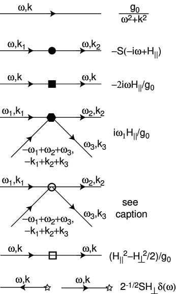
Figure 1: Propagator and vertices appearing in the calculation to the order needed. The weight of the fifth term is $(\vec{k}_{2}\cdot\vec{k}_{3}+\omega_{2}\omega_{3}+\vec{k}_{1}\cdot(\vec{k}_{2}+\vec{k_{3}}-\vec{k}_{1})+\omega_{1}(\omega_{2}+\omega_{3}-\omega_{1}))/(4g_{0})$.

First, we recall the results for the bulk response, in the absence of the impurity. The free energy is expanded as in (10), and this leads to the diagrams in Fig 2 to order $g_{0}^{0}$.

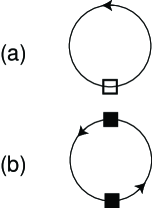
Figure 2: Diagrams for the bulk susceptibilities to order $g_{0}^{0}$.

There is no bulk linear dependence on $H_{\alpha}$ to all orders in $g_{0}$, and hence $m=0$ in the absence of the impurity. To quadratic order in $H_{\alpha}$ we have the bulk susceptibilities (per unit volume)

$$\chi_{\perp,\text{b}} = \frac{1}{g_{0}}+(\ref{figbulk}a)$$

$$(\ref{figbulk}a) = -T\sum_{\omega_{n}\neq 0}\int\frac{d^{d}k}{(2\pi)^{d}}\frac{1}{\omega_{n}^{2}+k^{2}}$$ (51)

$$= -2T^{d-1}\mathcal{J}_{1}(2\pi)^{d-2}\zeta(2-d)$$

and

$$\chi_{\parallel,\text{b}} = (\ref{figbulk}a)+(\ref{figbulk}b)$$

$$(\ref{figbulk}a) = 2T\sum_{\omega_{n}\neq 0}\int\frac{d^{d}k}{(2\pi)^{d}}\frac{1}{\omega_{n}^{2}+k^{2}}$$

$$= 4T^{d-1}\mathcal{J}_{1}(2\pi)^{d-2}\zeta(2-d)$$

$$(\ref{figbulk}b) = -4T\sum_{\omega_{n}\neq 0}\int\frac{d^{d}k}{(2\pi)^{d}}\frac{\omega_{n}^{2}}{(\omega_{n}^{2}+k^{2})^{2}}$$ (52)

$$= -8T^{d-1}\mathcal{J}_{2}(2\pi)^{d-2}\zeta(2-d),$$

where

$$\mathcal{J}_{a}\equiv\frac{\Gamma(a-d/2)}{(4\pi)^{d/2}\Gamma(a)}.$$ (53)

As discussed in Section III, all intermediate Matsubara frequencies in all diagrams in this appendix are summed only over non-zero values; the integration over the zero Matsubara frequency modes leads to (11). There are no infrared divergences in any graph (because of the summation over non-zero Matsubara frequencies), while ultraviolet divergences appear in individual graphs for $d\geq 1$. We also list the expressions for the individual graphs obtained in the dimensional regularization method, obtained by analytic continuation from the $d<1$ region—these will be useful in our renormalization group analysis. The dimensionally-regularized expressions ware obtained by first performing the momentum integrations, and the frequency summations are then naturally expressed in terms of the Riemann zeta function $\zeta(s)$. There are also many sensitive cancellations in the ultraviolet divergences of the various graphs considered in this appendix, and these will appear as cancellation of poles in the dimensionally regularized expressions. In Section III we have also considered the expressions of this appendix directly in $d=2$ without dimensional regularization, and these results illustrate the cancellation of ultraviolet divergences upon expression of the results in terms of physical observables.

The application of the perturbation theory towards computation of physical properties of the impurity in different regimes will be presented in separate subsections below.

A.1 Impurity susceptibility at $T>0$

We first address the computation of the impurity magnetic susceptibility, $\chi_{\text{imp}}$ at non-zero temperatures.

The diagrams for the perturbative expressions for the impurity contributions to the quantities in (10) are shown in Figs 3-5.

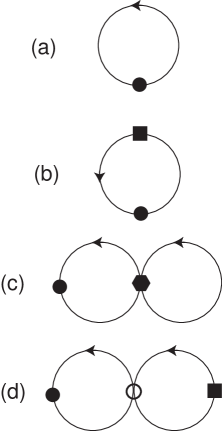
Figure 3: Diagrams contributing to $m$ to order $g_{0}^{2}$.

Now there is a contribution to linear order in $H_{\parallel}$, and Fig 3 yields the following expressions for $m$:

$$m = S+(\ref{figm}a)+(\ref{figm}b)+(\ref{figm}c)+(\ref{figm}d)$$

$$(\ref{figm}a) = -Sg_{0}T\sum_{\omega_{n}\neq 0}\int\frac{d^{d}k}{(2\pi)^{d}}\frac{1}{\omega_{n}^{2}+k^{2}}$$

$$= -2Sg_{0}T^{d-1}\mathcal{J}_{1}(2\pi)^{d-2}\zeta(2-d)$$

$$(\ref{figm}b) = 2Sg_{0}T\sum_{\omega_{n}\neq 0}\int\frac{d^{d}k}{(2\pi)^{d}}\frac{\omega_{n}^{2}}{(\omega_{n}^{2}+k^{2})^{2}}$$

$$= 4Sg_{0}T^{d-1}\mathcal{J}_{2}(2\pi)^{d-2}\zeta(2-d)$$

$$(\ref{figm}c) = -2Sg_{0}^{2}T^{2}\left[\sum_{\omega_{n}\neq 0}\int\frac{d^{d}k_{1}}{(2\pi)^{d}}\frac{\omega_{n}^{2}}{(\omega_{n}^{2}+k_{1}^{2})^{2}}\right]$$

$$~{}~{}~{}~{}~{}~{}~{}~{}~{}~{}~{}~{}\times\left[\sum_{\epsilon_{n}\neq 0}\int\frac{d^{d}k_{2}}{(2\pi)^{d}}\frac{1}{\epsilon_{n}^{2}+k_{2}^{2}}\right]$$

$$= -8Sg_{0}^{2}T^{2d-2}\mathcal{J}_{1}\mathcal{J}_{2}\left[(2\pi)^{d-2}\zeta(2-d)\right]^{2}$$

$$(\ref{figm}d) = 4Sg_{0}^{2}T^{2}\left[\sum_{\omega_{n}\neq 0}\int\frac{d^{d}k}{(2\pi)^{d}}\frac{\omega_{n}^{2}}{(\omega_{n}^{2}+k^{2})^{2}}\right]^{2}$$ (54)

$$= 16Sg_{0}^{2}T^{2d-2}\mathcal{J}_{2}^{2}\left[(2\pi)^{d-2}\zeta(2-d)\right]^{2}.$$

Figure 4: Diagram contributing to $\chi_{\perp,\text{imp}}$ to order $g_{0}^{2}$ at $T>0$.

Similarly, for $\chi_{\perp,\text{imp}}$ we only have the diagram in Fig 4 which yields:

$$\chi_{\perp,\text{imp}} = (\ref{figperp})$$

$$(\ref{figperp}) = S^{2}g_{0}^{2}T\sum_{\omega_{n}\neq 0}\int\frac{d^{d}k_{1}}{(2\pi)^{d}}\frac{d^{d}k_{2}}{(2\pi)^{d}}\frac{\omega_{n}^{2}}{(\omega_{n}^{2}+k_{1}^{2})^{2}}$$ (55)

$$~{}~{}~{}~{}~{}~{}~{}~{}~{}~{}~{}~{}~{}~{}\times\frac{1}{(\omega_{n}^{2}+k_{2}^{2})}$$

$$= 2S^{2}g_{0}^{2}T^{2d-3}\mathcal{J}_{1}\mathcal{J}_{2}(2\pi)^{2d-4}\zeta(4-2d).$$

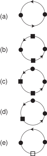
Figure 5: Diagrams contributing to $\chi_{\parallel,\text{imp}}$ to order $g_{0}^{2}$.

Finally, for $\chi_{\parallel,\text{imp}}$, we have the diagrams in Fig 5, from which we obtain:

$$\chi_{\parallel,\text{imp}} = (\ref{figpar}a)+(\ref{figpar}b)+(\ref{figpar}c)+(\ref{figpar}d)+(\ref{figpar}e)$$

$$(\ref{figpar}a) = S^{2}g_{0}^{2}T\sum_{\omega_{n}\neq 0}\int\frac{d^{d}k_{1}}{(2\pi)^{d}}\frac{d^{d}k_{2}}{(2\pi)^{d}}\frac{1}{(\omega_{n}^{2}+k_{1}^{2})}$$

$$~{}~{}~{}~{}~{}~{}~{}~{}~{}~{}~{}~{}~{}~{}\times\frac{1}{(\omega_{n}^{2}+k_{2}^{2})}$$

$$= 2S^{2}g_{0}^{2}T^{2d-3}\mathcal{J}_{1}^{2}(2\pi)^{2d-4}\zeta(4-2d)$$

$$(\ref{figpar}b) = 4S^{2}g_{0}^{2}T\sum_{\omega_{n}\neq 0}\int\frac{d^{d}k_{1}}{(2\pi)^{d}}\frac{d^{d}k_{2}}{(2\pi)^{d}}\frac{\omega_{n}^{4}}{(\omega_{n}^{2}+k_{1}^{2})^{2}}$$

$$~{}~{}~{}~{}~{}~{}~{}~{}~{}~{}~{}~{}~{}~{}\times\frac{1}{(\omega_{n}^{2}+k_{2}^{2})^{2}}$$

$$= 8S^{2}g_{0}^{2}T^{2d-3}\mathcal{J}_{2}^{2}(2\pi)^{2d-4}\zeta(4-2d)$$

$$(\ref{figpar}c) = 8S^{2}g_{0}^{2}T\sum_{\omega_{n}\neq 0}\int\frac{d^{d}k_{1}}{(2\pi)^{d}}\frac{d^{d}k_{2}}{(2\pi)^{d}}\frac{\omega_{n}^{4}}{(\omega_{n}^{2}+k_{1}^{2})^{3}}$$

$$~{}~{}~{}~{}~{}~{}~{}~{}~{}~{}~{}~{}~{}~{}\times\frac{1}{(\omega_{n}^{2}+k_{2}^{2})}$$

$$= 16S^{2}g_{0}^{2}T^{2d-3}\mathcal{J}_{3}\mathcal{J}_{1}(2\pi)^{2d-4}\zeta(4-2d)$$

$$(\ref{figpar}d) = -8S^{2}g_{0}^{2}T\sum_{\omega_{n}\neq 0}\int\frac{d^{d}k_{1}}{(2\pi)^{d}}\frac{d^{d}k_{2}}{(2\pi)^{d}}\frac{\omega_{n}^{2}}{(\omega_{n}^{2}+k_{1}^{2})^{2}}$$

$$~{}~{}~{}~{}~{}~{}~{}~{}~{}~{}~{}~{}~{}~{}\times\frac{1}{(\omega_{n}^{2}+k_{2}^{2})}$$

$$= -16S^{2}g_{0}^{2}T^{2d-3}\mathcal{J}_{1}\mathcal{J}_{2}(2\pi)^{2d-4}\zeta(4-2d)$$

$$(\ref{figpar}e) = -2S^{2}g_{0}^{2}T\sum_{\omega_{n}\neq 0}\int\frac{d^{d}k_{1}}{(2\pi)^{d}}\frac{d^{d}k_{2}}{(2\pi)^{d}}\frac{\omega_{n}^{2}}{(\omega_{n}^{2}+k_{1}^{2})^{2}}$$ (56)

$$~{}~{}~{}~{}~{}~{}~{}~{}~{}~{}~{}~{}~{}~{}\times\frac{1}{(\omega_{n}^{2}+k_{2}^{2})}$$

$$= -4S^{2}g_{0}^{2}T^{2d-3}\mathcal{J}_{1}\mathcal{J}_{2}(2\pi)^{2d-4}\zeta(4-2d)$$

A.2 Local susceptibility at $T>0$

The response to a field applied only near the impurity site can be computed as in Appendix A.2. Only the graphs in Fig 3a and  5a now contribute, and we have therefore

$$m_{\text{loc}} = S+(\ref{figm}a)$$

$$\chi_{\parallel,\text{loc}} = (\ref{figpar}a)$$

$$\chi_{\perp,\text{loc}} = 0$$ (57)

where the values of the respective graphs are as specified in (54) and (56).

A.3 Spin correlations at $T=0$

The methods above can also be extended to obtain impurity spin correlations at $T=0$ and $g_{0}=g_{c}$. As long as we restrict ourselves to rotationally invariant correlation functions, direct perturbation theory in $g_{0}$ is free of infrared divergences.

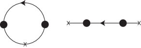
Figure 6: Lowest order diagram contributing to the correlator in (58) which depends upon the presence of the impurity. The $X$’s denote external sources for the fields.

For the impurity spin correlation in (39), the first corrections which depend upon the presence of the impurity do not appear until order $g_{0}^{3}$: these arise from the graphs shown in Fig 6 and lead to the following expression:

$$\left\langle N_{\alpha}(x=0,\tau)N_{\alpha}(x=0,0)\right\rangle=1+$$

$$~{}~{}2g_{0}^{3}S^{2}\int\frac{d\omega}{2\pi}\frac{d^{d}k_{1}}{(2\pi)^{d}}\frac{d^{d}k_{2}}{(2\pi)^{d}}\frac{d^{d}k_{3}}{(2\pi)^{d}}$$

$$~{}~{}~{}~{}\times\frac{\omega^{2}(1-\cos(\omega\tau))}{(\omega^{2}+k_{1}^{2})(\omega^{2}+k_{3}^{2})(\omega^{2}+k_{3}^{2})}+\ldots.$$ (58)

Here the ellipses denote numerous lower-order terms which do not depend upon the presence of the impurity and hence are the same at $x=0$ and $x\neq 0$; the first term which breaks translational invariance is shown in (58). The integrals in (58) can be easily evaluated in dimensional regularization, and the second term in (58) equals

$$-\frac{2g_{0}^{3}S^{2}[\Gamma((2-d)/2)]^{3}\Gamma(3d-3)\cos(3\pi(d-1)/2)}{(4\pi)^{3d/2}\pi\tau^{3d-3}}$$ (59)

Picking out the pole in $\epsilon$ in (59), we immediately obtain (38).

A.4 Response to a field at $T=0$

As discussed in Section III.3, we need the impurity contribution to the free energy in the presence of an applied transverse magnetic field $H_{\perp}$, $\mathcal{F}_{\text{imp}}(H_{\perp})$. We will see that the response is singular as $H_{\perp}\rightarrow 0$. The singularity can be cutoff by an easy-axis spin anisotropy, and for completeness, we perform the computation in the presence of such an anisotropy. So we modify the action by

$$\mathcal{S}_{b}[N_{\alpha}]\rightarrow\mathcal{S}_{b}[N_{\alpha}]-\frac{D}{2}\int d^{d}x\int_{0}^{1/T}d\tau N_{z}^{2}.$$ (60)

Because we are now computing the free energy to all orders in the applied field, the Feynman graph expansion is quite tedious, and we will be satisfied by obtaining the result only to order $g_{0}$. The computation is done most simply using the Cartesian components $\sim(\psi+\psi^{\ast},-i(\psi-\psi^{\ast}))$, and to leading order in $g_{0}$, only the graph shown in Fig 7 contributes.

Figure 7: Diagram contributing to the free energy $\mathcal{F}(H_{\perp})$ to order $g_{0}$. at $T=0$. The propagator represents the $x$ component of $N_{\alpha}$ and includes the open square vertex in Fig 1 to all orders in $H_{\perp}$, along with the easy-axis anisotropy in (60); it equals $g_{0}/(\omega^{2}+k^{2}+D+H_{\perp}^{2})$.

Note that this diagram did not appear in the computation at $T>0$ because of the restriction there to summation over non-zero Matsubara frequencies and the delta function in frequency associated with the vertex in Fig 7; the leading term in $\chi_{\perp,\text{imp}}$ was of order $g_{0}^{2}$ at $T>0$. From the diagram in Fig 7 we obtain

$$\mathcal{F}_{\text{imp}}(H_{\perp}) = -\frac{g_{0}H_{\perp}^{2}S^{2}}{2}\int\frac{d^{d}k}{(2\pi)^{d}}\frac{1}{k^{2}+D+H_{\perp}^{2}}$$ (61)

$$= -\frac{g_{0}H_{\perp}^{2}S^{2}}{2}\mathcal{J}_{1}(D+H_{\perp}^{2})^{(d-2)/2}.$$

This graph has a log singularity in $d=2$. The same logarithm appeared in a different manner in the $T>0$ computation: it was present in Fig 3a. Ultimately it is only $\chi_{\text{imp}}$ that is physically measurable at $T>0$, and it is clear now that the logarithm appears in different places depending upon the different organizations of perturbation theory at $T=0$ and $T>0$.

Appendix B Perturbation theory for general $\gamma$

The computations elsewhere in this paper have been limited to the case in which the coupling between the impurity spin and the bulk antiferromagnetic spin fluctuations, $\gamma$, has effectively been sent to infinity. We have argued that this limit appears naturally in the vicinity of the quantum critical point. This appendix will consider the general $\gamma$ case, and consider the extent to which the low $T$ properties away from the critical point are independent of the value of $\gamma$.

We shall be concerned here with the partition function

$$\mathcal{Z}_{\gamma}=\int\mathcal{D}N_{\alpha}(x,\tau)\delta\left(N_{\alpha}^{2}-1\right)\mathcal{D}n_{\alpha}\delta(n_{\alpha}^{2}-1)$$

$$~{}~{}~{}~{}~{}~{}~{}~{}~{}~{}~{}~{}~{}~{}\times\exp\left(-\mathcal{S}_{\text{b}}[N_{\alpha}]-\mathcal{S}_{\text{imp},\gamma}\right)$$

$$\mathcal{S}_{\text{imp},\gamma}=\int_{0}^{1/T}d\tau\bigg{[}iSA_{\alpha}(n)\frac{dn_{\alpha}(\tau)}{d\tau}$$

$$~{}~{}~{}~{}~{}~{}~{}~{}~{}~{}~{}~{}~{}~{}~{}~{}~{}~{}~{}-\gamma SN_{\alpha}(x=0,\tau)n_{\alpha}(\tau)\bigg{]},$$ (62)

where $\mathcal{S}_{\text{b}}[N_{\alpha}]$ is as in (8), and $A_{\alpha}(n)$ is defined by (7). In principle, it is possible to generate an expansion in powers of $g_{0}$, with each term containing its exact dependence on $\gamma$ and $S$; this requires an exact treatment of the impurity spin fluctuations, and this can be done by the method described in Appendix C of I. Here, we shall use the method described above in Section A with a parametrization similar to (47) applied also to $n_{\alpha}$. By this method, it is not difficult to obtain results order-by-order in $g_{0}$, dropping only diagrams with a ‘tadpole’ factor of the impurity spin propagator (i.e. with a simple closed loop of the impurity spin propagator)—these are easily seen to have a prefactor of $e^{-\gamma/T}$ (we assume, without loss of generality, that $\gamma>0$).

We now present results to order $g_{0}$ for the impurity spin susceptibility at $T>0$, computed above in Appendix A.1. We will omit all details and merely present final results to leading order in $g_{0}$. Dropping terms with a pre-factor of $e^{-\gamma/T}$, we found

$$m=S-\gamma^{2}Sg_{0}T\sum_{\omega_{n}\neq 0}\int\frac{d^{d}k}{(2\pi)^{d}}\Biggl{[}$$

$$\frac{1}{(\omega_{n}^{2}+k^{2})(-i\omega_{n}+\gamma)^{2}}+\frac{2i\omega_{n}}{(\omega_{n}^{2}+k^{2})^{2}(-i\omega_{n}+\gamma)}\Biggr{]}$$

$$\chi_{\parallel,\text{imp}}=2\gamma Sg_{0}T\sum_{\omega_{n}\neq 0}\int\frac{d^{d}k}{(2\pi)^{d}}\Biggl{[}$$

$$\frac{4\omega_{n}^{2}}{(\omega_{n}^{2}+k^{2})^{3}}-\frac{1}{(\omega_{n}^{2}+k^{2})^{2}}+\frac{\gamma}{(\omega_{n}^{2}+k^{2})(-i\omega_{n}+\gamma)^{3}}$$

$$+\frac{\gamma}{(\omega_{n}^{2}+k^{2})^{2}(-i\omega_{n}+\gamma)}+\frac{2i\gamma\omega_{n}}{(\omega_{n}^{2}+k^{2})^{2}(-i\omega_{n}+\gamma)^{2}}$$

$$-\frac{4\gamma\omega_{n}^{2}}{(\omega_{n}^{2}+k^{2})^{3}(-i\omega_{n}+\gamma)}\Biggr{]}$$

$$\chi_{\perp,\text{imp}}=\gamma Sg_{0}T\sum_{\omega_{n}\neq 0}\int\frac{d^{d}k}{(2\pi)^{d}}\Biggl{[}\frac{1}{(\omega_{n}^{2}+k^{2})^{2}}$$

$$~{}~{}~{}~{}~{}~{}-\frac{\gamma}{(\omega_{n}^{2}+k^{2})^{2}(-i\omega_{n}+\gamma)}\Biggr{]}.$$ (63)

It is now easy to check that the $\gamma\rightarrow\infty$ limit of these expressions is finite, and indeed agrees precisely with the order $g_{0}$ results for $\chi_{\text{imp}}$ obtained in Section III.1 and Appendix A.1; this is a non-trivial check of our computations. Evaluation of the frequency summations in (63) is a tedious but straightforward exercise. After this, we combine the results using (11), and evaluate the momentum integrals at low $T$ as in Section III, while keeping $\gamma$ finite; in the limit of $T\ll\gamma,\Lambda$ we obtain in $d=2$

$$\chi_{\rm imp} = \frac{S^{2}}{3T}\Biggl{[}1+\left(\frac{T}{\pi\rho_{s}}-\frac{T^{2}}{\pi S\rho_{s}\gamma}\right)\ln\left(\frac{\Lambda}{T}\right)\Biggr{]}.$$ (64)

Notice that the co-efficient of the $(1/\rho_{s})\ln(1/T)$ is independent of $\gamma$, and that it agrees with (4). Also, at finite $\gamma$, the $T\ln(1/T)$ term does acquire a non-universal $\gamma$-dependent correction.

Appendix C Low temperature properties in $d=3$

This appendix briefly describes the extension of our results to $d=3$. The bulk quantum critical point in $d=3$ does not satisfy strong scaling properties, and so we will not consider it here. We will focus only on the low $T$ properties within the magnetically ordered state, well away from any quantum critical point.

Magnetic long-range order is present for a finite range of $T>0$, and so the magnetic response remains anisotropic as $T\rightarrow 0$. The quantities $m$, $\chi_{\perp,\text{imp}}$, $\chi_{\parallel,\text{imp}}$ retain their separate physical identities, and can be measured separately.

The low $T$ expansions for $m$, $\chi_{\perp,\text{imp}}$, $\chi_{\parallel,\text{imp}}$ are obtained as in Appendix A. Indeed, now we need not separate the $\omega_{n}=0$ and the $\omega_{n}\neq 0$ modes as there is long-range order for $T>0$: the expressions in Appendix A can therefore be used here, after converting all frequency summations to run over both zero and non-zero values of Matsubara frequencies. In this manner, (16) is modified to

$$m = S\left[1-\frac{T}{\rho_{s}}\left\{\int\frac{d^{3}k}{(2\pi)^{3}}\frac{1}{4T^{2}\sinh^{2}(k/(2T))}\right\}\right.$$ (65)

$$~{}~{}~{}~{}\times\left\{1+\frac{T}{\rho_{s}}\int\frac{d^{3}p}{(2\pi)^{3}}\left(\frac{1}{pT(e^{p/T}-1)}\right.\right.$$

$$~{}~{}~{}~{}~{}~{}~{}~{}~{}~{}~{}~{}~{}~{}~{}~{}~{}~{}~{}\left.\left.\left.-\frac{1}{4T^{2}\sinh^{2}(p/(2T))}\right)\right\}\right].$$

Evaluating the momentum integrations, and re-inserting factors of $c$, we obtain

$$m=S\left(1-\frac{T^{2}}{6c\rho_{s}}+\frac{T^{4}}{72c^{2}\rho_{s}^{2}}+\ldots\right).$$ (66)

Interestingly, the expression (66) can also be obtained simply by setting $d=3$ in (18). For the finite $\gamma$ case, discussed in Appendix B, the $T^{2}$ term above remains unchanged, while the $T^{4}$ term does acquire $\gamma$-dependent corrections.

The results for $\chi_{\parallel,\text{imp}}$ and $\chi_{\perp,\text{imp}}$ now follow from (56) and (55). Setting $d=3$ in the dimensionally regularized expressions here, we find that the co-efficient of the universal $T^{3}$ term vanishes for both quantities. However, there are non-universal $T^{2}$ corrections for both $\chi_{\parallel,\text{imp}}$ and $\chi_{\perp,\text{imp}}$, and these have to be estimated directly from the expressions in (56) and (55): the frequency summations have to be evaluated first (including the zero Matsubara frequencies), and then the momentum integrations have to be evaluated with a finite cutoff.

Similar techniques apply to the response to a local field discussed in Appendix A.2. Now we obtain the universal correction

$$m_{\text{loc}}(T)-m_{\text{loc}}(0)=-\frac{ST^{2}}{12c\rho_{s}}$$ (67)

along with non-universal $T^{2}$ corrections to $\chi_{\perp,\text{loc}}$ and $\chi_{\parallel,\text{loc}}$. The factor of 2 difference between the $T^{2}$ terms in (67) and (66) is an interesting characteristic of the theory.

Appendix D Comment on Sushkov’s computation

It has been claimed by Sushkov sushkov that the Curie constant remains $\mathcal{C}_{1}=1/4$ for a $S=1/2$ impurity at the quantum critical point of an antiferromagnet. Here we show using the model of his paper that there is a perturbative correction to the impurity susceptibility, and that this implies an anomalous Curie constant. Of course, the possibility remains open that the $(3-d)$ and $(d-1)$ expansions both fail in $d=2$ near the critical point, but reasons for such a possible failure do not appear in Sushkov’s arguments.

Sushkov models the bulk spin fluctuations at the quantum critical point using a $S=1$ boson $t_{\alpha}$, as in Ref. bondops, . These bosons are coupled to the external magnetic field $H$ (assumed oriented along the $z$ axis) and to the impurity moment $\hat{S}_{\alpha}$. This gives us the model considered by Sushkov:

$$\mathcal{H} = \mathcal{H}_{0}+\mathcal{H}_{1}$$

$$\mathcal{H}_{0} = \sum_{{\bf k}}\sum_{m=0,\pm 1}(\varepsilon({\bf k})-mH)t^{\dagger}_{m}({\bf k})t_{m}({\bf k})-H\hat{S}_{z}$$

$$\mathcal{H}_{1} = \lambda{\phi}_{\alpha}\hat{S}_{\alpha}$$ (68)

where ${\bf k}$ is the momentum of the $t_{\alpha}$ bosons with energy $\varepsilon({\bf k})$, and

$${\phi}_{\alpha}=\sum_{{\bf k}}\frac{1}{\sqrt{2\varepsilon({\bf k})}}({t}_{\alpha}({\bf k})+{t}_{\alpha}^{\dagger}({\bf k}))$$ (69)

and

$$t_{x} = (t_{1}+t_{-1})/\sqrt{2}$$

$$t_{y} = i(t_{1}-t_{-1})/\sqrt{2}$$

$$t_{z} = t_{0}$$ (70)

It can be checked that $H$ couples to the total spin, which commutes with the Hamiltonian.

Now we compute the free energy, $\mathcal{F}$, in a power series in $\lambda$ in arbitrary $H$. To second order in $\lambda$, this is done by the familiar formula

$$\mathcal{F}=-T\ln{\rm Tr}e^{-\mathcal{H}_{0}/T}$$

$$-T\int_{0}^{1/T}\!\!d\tau\int_{0}^{\tau}d\tau_{1}\frac{{\rm Tr}\left(e^{-\mathcal{H}_{0}/T}\mathcal{H}_{1}(\tau)\mathcal{H}_{1}(\tau_{1})\right)}{{\rm Tr}e^{-\mathcal{H}_{0}/T}}$$ (71)

where

$$\mathcal{H}_{1}(\tau)=e^{\mathcal{H}_{0}\tau}\mathcal{H}_{1}e^{-\mathcal{H}_{0}\tau}$$ (72)

Everything in (71) and (72) can be evaluated analytically by simple means, and then we can perform the integrals over $\tau$ and $\tau_{1}$ - this was done using the computer program Mathematica for arbitrary $H$ and $S$, without using any diagrammatic perturbation theory. Finally, we can expand the result in powers of $H$ and obtain for the impurity susceptibility

$$\chi_{\rm imp}=\frac{S(S+1)}{3T}+\frac{2\lambda^{2}S(S+1)}{3T^{2}}\sum_{{\bf k}}\frac{e^{\varepsilon({\bf k})/T}}{\varepsilon({\bf k})^{2}(e^{\varepsilon({\bf k})/T}-1)^{2}}$$ (73)

This result agrees precisely with that obtained using a diagrammatic approach in I. It disagrees with that of Sushkov, who did not obtain any correction to the first free moment term—he does not appear to have considered the cross-correlation between the bulk magnetization of the $t_{\alpha}$ and the impurity magnetization. Note that this disagreement appears already at the level of bare perturbation theory, and does not involve any of the subtleties associated with approaching the scaling limit at the critical point in the $\epsilon$ or $1/N$ expansions.

In the quantum disordered regime above the paramagnetic phase, we can model $\varepsilon({\bf k})=\sqrt{c^{2}{\bf k}^{2}+\Delta_{T}^{2}}$, where $\Delta_{T}\sim\Delta>0$ is the spin gap vbs ; bondops ; here (73) predicts a contribution of order $e^{-\Delta/T}$ to the susceptibility, and so the moment is indeed precisely quantized at $S$.

However, the quantum critical region vbs we have $\Delta_{T}\sim T$, and then (73) yields a contribution to the susceptibility of order $\lambda^{2}T^{d-4}$. For $d<3$, the dimensionless combination $\lambda^{2}T^{d-3}$ approaches a universal value at the fixed point, and a universal irrational correction to the Curie term applies, as shown in much detail in I.

References

(1) S. Sachdev, C. Buragohain and M. Vojta,
Science 286, 2479 (1999).
(2) M. Vojta, C. Buragohain, and S. Sachdev,
Phys. Rev. B 61, 15152 (2000).
(3) O. P. Sushkov, Phys. Rev. B 62, 12135
(2000).
(4) S. Sachdev, M. Troyer, and M. Vojta, Phys. Rev. Lett.
86, 2617 (2001).
(5) M. Troyer, Prog. Theor. Phys. Supp. 145, 326 (2002).
(6) K. H. Höglund and A. W. Sandvik,
cond-mat/0302273.
(7) A. W. Sandvik, Phys. Rev. Lett. 89, 177201 (2002);
O. P. Vajk and M. Greven, Phys. Rev. Lett. 89, 177202
(2002).
(8) O. P. Vajk, P. K. Mang, M. Greven, P. M. Gehring, and
J. W. Lynn, Science 295, 1691 (2002).
(9) L. Zhu and Q. Si, Phys. Rev. B 66, 024426
(2002).
(10) G. Zaránd and E. Demler,
Phys. Rev. B 66, 024427 (2002).
(11) N. Katoh and M. Imada, J. Phys. Soc. Jpn.
63, 4529 (1994); J. Tworzydlo, O. Y. Osman, C. N. A. van
Duin, J. Zaanen, Phys. Rev. B 59, 115 (1999); M. Matsumoto,
C. Yasuda, S. Todo, and H. Takayama, Phys. Rev. B 65, 014407
(2002).
(12) N. Nagaosa, Y. Hatsugai, and
M. Imada, J. Phys. Soc. Jpn 58, 978 (1989).
(13) A. L. Chernyshev, Y. C. Chen, and A. H. Castro Neto,
Phys. Rev. B 65, 104407 (2002).
(14) A. J. Millis, D. K. Morr, and J. Schmalian, Phys. Rev. Lett. 87,
167202 (2001).
(15) E. Brezin and J. Zinn-Justin, Phys. Rev. B 14,
3110 (1976).
(16) S. Sachdev, Quantum Phase Transitions,
Cambridge University Press, Cambridge (1999).
(17) P. Hasenfratz and F. Niedermayer, Z. Phys. B 92, 91 (1993).
(18) A. V. Chubukov, S. Sachdev, and J. Ye,
Phys. Rev. B 49, 11919 (1994).
(19) S. Das Sarma, S. Sachdev and L. Zheng, Phys. Rev. B 58, 4672 (1998).
(20) A. Sandvik, private communication.
(21) S. Sachdev and R. N. Bhatt, Phys. Rev. B 41,
9323 (1990).