On the Nature of the X-ray Emission from the Accreting Millisecond Pulsar SAX J1808.4$-$3658

Abstract

The pulse profiles of the accreting X-ray millisecond pulsar SAX J1808.4$-$3658 at different energies are studied. The two main emission component, the black body and the Comptonized tail that are clearly identified in the time-averaged spectrum, show strong variability with the first component lagging the second one. The observed variability can be explained if the emission is produced by Comptonization in a hot slab (radiative shock) of Thomson optical depth $\sim$ 0.3–1 at the neutron star surface. The emission patterns of the black body and the Comptonized radiation are different: a “knife”– and a “fan”–like, respectively. We construct a detailed model of the X-ray production accounting for the Doppler boosting, relativistic aberration and gravitational light bending in the Schwarzschild spacetime. We present also accurate analytical formulae for computations of the light curves from rapidly rotating neutron stars using formalism recently developed by Beloborodov (2002). Our model reproduces well the pulse profiles at different energies simultaneously, corresponding phase lags, as well as the time-averaged spectrum. We constrain the compact star mass to be bounded between $1.2$ and $1.6{\rm M_{\odot}}$. By fitting the observed profiles, we determine the radius of the compact object to be $R\sim 11$ km if $M=1.6{\rm M_{\odot}}$, while for $M=1.2{\rm M_{\odot}}$ the best-fitting radius is $\sim 6.5$ km, indicating that the compact object in SAX J1808.4$-$3658 can be a strange star. We obtain a lower limit on the inclination of the system of $65\degr$.

1 Introduction

Discovery of coherent oscillations with frequencies in the 300–600 Hz range during X-ray bursts from a number of low-mass X-ray binaries (see Strohmayer & Bildsten 2003 for a review) has triggered the efforts to use the information on the amplitude of variability and the folded pulse shape to put constraints on the compactness of the neutron star and thus its equation of state as well as the emission pattern from the neutron star surface (e.g. Miller & Lamb 1998). However, a rather limited photon statistics does not allow to reach a high accuracy (Strohmayer et al. 1997; Nath, Strohmayer & Swank 2002; Muno, Özel & Chakrabarty 2002).

The millisecond coherent pulsations discovered in the persistent emission of the four sources: SAX J1808.4$-$3658 (with the period $P=2.5$ ms; Wijnands & van der Klis 1998a), XTE J1751$-$305 ($P=2.3$ ms; Markwardt et al. 2002), XTE J0929$-$314 ($P=5.4$ ms; Galloway et al. 2002) and XTE J1807$-$294 ($P=5.25$ ms; Markwardt, Smith & Swank 2003) allow one to increase the statistics by folding the profile over a longer observational period (days rather than seconds in the X-ray burst oscillations). Thus, for example, SAX J1808.4$-$3658 showed coherent pulsations with rms amplitude of 5–7 per cent during its April 1998 outburst (Cui et al. 1998) with almost constant shape of its energy spectrum (Gilfanov et al. 1998) and very similar pulse profiles. The pulse profiles of SAX J1808.4$-$3658 show strong energy dependence with soft photons lagging behind the hard ones (soft phase lags, see Cui et al. 1998). By analysing the phase-resolved spectra, Gierliński, Done & Barret (2002) showed that this results from the fact that the two main spectral components, a soft black body and a hard Comptonized, vary out of phase with the first lagging the last one. While the variations of the black body flux can be described by a single sine wave, the pulse of the hard Comptonized component is strongly skewed. Gierliński et al. (2002) suggested that the Doppler boosting can play a role in changing the shape of the profile.

The radiation pattern of standard accreting X-ray pulsars is influenced by strong magnetic field $B\sim 10^{12}$ G. On the other hand, the magnetic field of the accreting millisecond pulsars in low mass X-ray binaries is much weaker, $B=10^{8}$–$10^{9}$ G (see e.g. Wijnands & van der Klis 1998a; Psaltis & Chakrabarty 1999), and does not affect significantly properties of the emitted radiation. Thus these sources can also serve as laboratories for studying radiative processes at the surface of weakly-magnetized neutron stars.

In this paper, we construct a detailed model for the X-ray emission from the surface of a rapidly rotating neutron star accounting for relativistic effects. We compare the model with the data on SAX J1808.4$-$3658 and put constraints on the inclination of the system, the position of the emitting region relative to the rotational pole and its emission pattern as well as the stellar radius. The data used for the analysis are described in § 2. The model and useful analytical formulae for light curve calculations are presented in § 3. The main results are given in § 4. The discussion and the summary are given in § 5 and § 6, respectively.

2 Data

We study the data obtained by the Rossi X-ray Timing Explorer (RXTE) during the April 1998 outburst of SAX J1808.4$-$3658, using ftools 5.2. To improve the statistics we average the data between 1998 April 11 and 29 (resulting in 118 ks of data). For spectral fitting we extract the Proportional Counter Array (PCA) spectra from all five detectors, top layer only, and use the data in 3–20 keV energy band. We also extract spectra from High-Energy X-ray Timing Experiment (HEXTE) in the 20–150 keV band, from clusters 0 and 1. We constructed the energy-dependent pulse profiles from the PCA data (all detectors, all layers) by following the procedure described in Cui et al. (1998) and Gierliński et al. (2002) correcting the photon arrival times for orbital motions of the pulsar and the spacecraft. For pulse profile fitting we created two folded light curves in 16 phase bins, for energies 3–4 keV and 12–18 keV. The statistical uncertainties are about the same as uncertainties in the background, resulting in errors of 0.2 per cent and 0.3 per cent, respectively, in the count rate in the two considered energy bands.

3 Model

3.1 Calculational method

Accreting matter following the magnetic field lines close to the neutron star is stopped in the very vicinity of the surface by radiation producing radiation dominated shock (Basko & Sunyaev 1976; Lyubarskii & Sunyaev 1982). For the source luminosity of a few percent of the Eddington luminosity (Gilfanov et al. 1998; Gierliński et al. 2002), the vertical (i.e. along the radial direction) extension of the shocked plasma is smaller than a characteristic horizontal size and certainly smaller than the stellar radius. The hard X-rays produced in the shock can irradiate the surrounding stellar surface, so that the black body emission region can cover a somewhat larger area. For our calculations we assume that all photons originate at the stellar surface (i.e. the height of the emitting region is set to zero).

We assume a circular spot and consider two extreme cases for the relative positions of the black body and the Comptonizing regions: (1) a homogeneous slab, i.e. the hot Comptonizing layer covering the whole black body spot, (2) a point–like Comptonizing region in the centre of a black body region.

In order to compute the light curve as observed by a distant observer, we first specify the radiation spectrum and angular dependence in the frame co-rotating with the star. We then make Lorentz transformation to obtain the radiation intensity in the non-rotating frame close to the stellar surface. At the final step, we follow photon trajectories in the Schwarzschild spacetime to infinity.

Let us now consider a star with an azimuthally symmetric surface radiation intensity $I^{\prime}(E^{\prime},\alpha^{\prime})$ that can vary over the surface, where $\alpha^{\prime}$ is the angle between an emitted photon and the local normal to the stellar surface. Let ${\rm d}S^{\prime}$ be a surface element (spot) at colatitude $\theta$ (see Fig. 1 for the geometry). The primed quantities correspond to the frame co-rotating with the spot. Let $\mn@boldsymbol{k}$ and $\mn@boldsymbol{n}$ be unit vectors pointing from the star centre towards the observer and the spot, respectively, and $i$ be the inclination of the spin axis. The inclination of the spot varies periodically

$$\cos\psi=\mn@boldsymbol{k}\cdot\mn@boldsymbol{n}=\cos i\ \cos\theta+\sin i\ \sin\theta\ \cos\phi,$$ (1)

where the phase $\phi=2\pi\nu t$, with $\nu$ being the pulsar frequency and $t=0$ is chosen when the spot is closest to the observer.

We compute the original direction of the photon $\mn@boldsymbol{k}_{0}$ near the stellar surface (which is transformed to $\mn@boldsymbol{k}$ at large distance from the star) assuming Schwarzschild geometry where photon orbits are planar:

$$\mn@boldsymbol{k}_{0}=[\sin\alpha\ \mn@boldsymbol{k}+\sin(\psi-\alpha)\ \mn@boldsymbol{n}]/\sin\psi,$$ (2)

where $\alpha$ is the angle between $\mn@boldsymbol{k}_{0}$ and $\mn@boldsymbol{n}$, i.e. $\cos\alpha=\mn@boldsymbol{k}_{0}\cdot\mn@boldsymbol{n}$.

The relation between $\alpha$ and $\psi$ (i.e. light bending) can be obtained by standard techniques (Pechenick, Ftaclas & Cohen 1983):

$$\psi=\int_{R}^{\infty}\frac{{\rm d}r}{r^{2}}\left[\frac{1}{b^{2}}-\frac{1}{r^{2}}\left(1-\frac{r_{g}}{r}\right)\right]^{-1/2},$$ (3)

where the impact parameter

$$b=\frac{R}{\sqrt{1-r_{g}/R}}\sin\alpha,$$ (4)

$r_{g}=2GM/c^{2}$ is the Schwarzschild radius, $M$ is the mass and $R$ is the radius of the compact star.

Figure 1: The geometry of the problem. Dotted curve shows the photon trajectory.

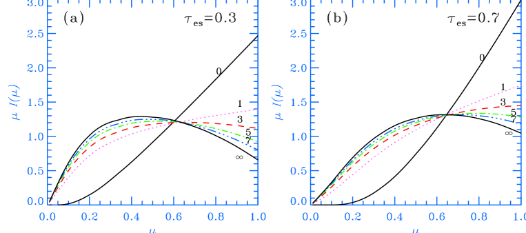
Figure 2: Angular distribution of the radiation flux (normalized as $\int\mu I(\mu)d\mu=1$) escaping from the top of an electron scattering slab of Thomson optical depth $\tau_{\rm es}=0.3$ (left) and $\tau_{\rm es}=0.7$ (right). Incident radiation from the bottom is a black body (intensity independent of the zenith angle $\arccos\mu$). Computations follow procedure described in Sunyaev & Titarchuk (1985). Different scattering orders are shown and marked by numbers. In the Comptonization process, scatterings also shift photons along the energy axis so that at a given energy one scattering order dominates (see Sunyaev & Titarchuk 1985; Poutanen & Svensson 1996).

The observed flux at energy $E$ is ${\rm d}F_{E}=I(E){\rm d}\Omega$, where $I(E)$ is the radiation intensity at the infinity and ${\rm d}\Omega$ is the solid angle occupied by ${\rm d}S^{\prime}$ on the observer’s sky. The solid angle can be expressed through the impact parameter

$${\rm d}\Omega=b\ {\rm d}b\ {\rm d}\varphi/D^{2},$$ (5)

where $D$ is the distance to the source and $\varphi$ is the azimuthal angle corresponding to rotation around $\mn@boldsymbol{k}$. The impact parameter $b$ depends on $\psi$ only, but not on $\varphi$.

The apparent area of the spot as measured by photon beams in the non-rotating frame near the stellar surface is ${\rm d}S=\delta\ {\rm d}S^{\prime}$ (see Terrell 1959; Lightman et al. 1975; Ghisellini 1999) and the relation between $\alpha$ and $\alpha^{\prime}$ is described by the relativistic aberration formula (for motions parallel to the spot surface)

$$\cos\alpha^{\prime}=\delta\ \cos\alpha,$$ (6)

where $\delta$ is the Doppler factor. Thus the spot area projected on to the plane perpendicular to the photon propagation direction, i.e. a photon beam cross-section, is Lorentz invariant (see e.g. Lightman et al. 1975; Lind & Blandford 1985):

$${\rm d}S\ \cos\alpha={\rm d}S^{\prime}\ \cos\alpha^{\prime}.$$ (7)

Representing ${\rm d}S=R^{2}\ {\rm d}\cos\psi\ {\rm d}\varphi$ and using equations (4) and (7) we get from (5)

$${\rm d}\Omega=\frac{{\rm d}S^{\prime}\cos\alpha^{\prime}}{D^{2}}\ \frac{1}{1-r_{g}/R}\ \frac{{\rm d}\cos\alpha}{{\rm d}\cos\psi}.$$ (8)

The Doppler factor can be expressed as follows

$$\delta=1/[\gamma(1-\beta\cos\xi)],$$ (9)

where $\gamma=(1-\beta^{2})^{-1/2}$ and $\beta=v/c$ is the spot velocity as measured in the non-rotating frame,

$$\beta=\frac{2\pi R}{c}\frac{\nu}{\sqrt{1-r_{g}/R}}\sin\theta=\beta_{\rm eq}\sin\theta.$$ (10)

Here $\beta_{\rm eq}$ is the velocity at the equator and $\xi$ is the angle between the spot velocity and $\mn@boldsymbol{k}_{0}$. The pulsar frequency is corrected here for the redshift $\sqrt{1-r_{g}/R}$. Using equation (2) it is easy to show that

$$\cos\xi=\frac{\mn@boldsymbol{\beta}}{\beta}\cdot\mn@boldsymbol{k}_{0}=\frac{\sin\alpha}{\sin\psi}\frac{\mn@boldsymbol{\beta}}{\beta}\cdot\mn@boldsymbol{k}=-\frac{\sin\alpha}{\sin\psi}\sin i\ \sin\phi\ .$$ (11)

In the case of a weak field and negligible bending the solid angle occupied by the spot is ${\rm d}\Omega={\rm d}S^{\prime}\cos\alpha^{\prime}/D^{2}$. In reality, this formula can be applied even when bending is significant since the relation between $\cos\alpha$ and $\cos\psi$ is close to linear (Beloborodov 2002),

$$\cos\alpha\approx r_{g}/R+(1-r_{g}/R)\cos\psi,$$ (12)

for a star with $R>2r_{g}$, so that ${\rm d}\cos\alpha/{\rm d}\cos\psi\approx 1-r_{g}/R$.

The radiation intensity observed at the infinity is $I(E)=(1-r_{g}/R)^{3/2}I_{0}(E_{0},\alpha)$, where $E/E_{0}=\sqrt{1-r_{g}/R}$ is the redshift (Misner, Thorn & Wheeler 1973) and the energy $E_{0}$ is measured in the non-rotating frame near the stellar surface. (In the actual calculations, one can neglect the redshift factor in all formulae for photon energies, since it is the same for the photons originating at the stellar surface.) Now we can make Lorentz transformation to the spot rest frame where we know the angular and energy distribution of the radiation field $I^{\prime}(E^{\prime},\alpha^{\prime})$. The intensities are related via $I_{0}(E_{0},\alpha)=\delta^{3}I^{\prime}(E^{\prime},\alpha^{\prime})$ with the Doppler shift given by $E_{0}=\delta\ E^{\prime}$.

Combining equations above we get the expression for the observed flux:

$${\rm d}F_{E}=\frac{\sqrt{1-r_{g}/R}}{D^{2}}\ \delta^{3}I^{\prime}\left(E^{\prime},\alpha^{\prime}\right)\frac{{\rm d}\cos\alpha}{{\rm d}\cos\psi}\ {\rm d}S^{\prime}\cos\alpha^{\prime},$$ (13)

with the visibility condition $\cos\alpha^{\prime}>0$. We account thus here for the special relativistic effects (Doppler boosting, relativistic aberration), the gravitational redshift and light bending in Schwarzschild geometry. In order to evaluate the flux at a given phase $\phi$, one first computes $\psi$ using equation (1), then inverting (3) gets $\alpha$ and substitutes the results into equations (11) and (9) to obtain the Doppler factor which is used later to compute $\alpha^{\prime}$ from equation (6). The light curve from the antipodal spot can be easily obtained by replacing in all formulae $\theta\rightarrow\pi-\theta$ and $\phi\rightarrow\pi+\phi$. We note here that the formalism outlined above neglects the time delays due to different photon paths (see Pechenick et al. 1983) which can be easily incorporated. However, they are negligible comparing to the pulsar period above a few ms.

For a spot of the finite size, the observed flux can be obtained by integrating over the (visible) spot area. On the other hand, if we know from the observations the black body flux $F_{\rm bb}$, its temperature $T_{\infty}$ and the distance to the source $D$, one can estimate the size of the (black body) emitting region. The “observed” radius of the spot $r_{\rm spot,\infty}=(F_{\rm bb}D^{2}/\sigma_{\rm SB}T_{\infty}^{4})^{1/2}$ should be corrected for the effects of gravitation and orientation (using a procedure described in § 3.3, see also Psaltis, Özel & DeDeo 2000) to obtain the actual spot area.

In our calculations of the model light curves for SAX J1808.4$-$3658 we use the distance $D=2.5$ kpc (in’t Zand et al. 2001), $T_{\infty}=0.66$ keV, and $r_{\rm spot,\infty}=2.4$ km (see Fig. 3 and Gierliński et al. 2002). Since the observed profiles from SAX J1808.4$-$3658 have almost sinusoidal shapes, they cannot be produced by two antipodal spots. Therefore, we compute the light curves from the primary spot (closest to the observer) only. We also neglect multiple images since neutron or strange stars have sizes larger than $1.5r_{g}$ (see e.g. Lattimer & Prakash 2001).

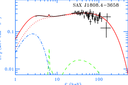
Figure 3: Time-averaged spectrum of SAX J1808.4$-$3658 as observed by RXTE. The model spectrum (solid curve) consists of a black body (dashes/dots), thermal Comptonization (dots), and Compton reflection with the iron line (dashes). Thermal Comptonization component (model thcomp in xspec; Zdziarski, Johnson & Magdziarz 1996) has a best-fitting photon spectral slope $\Gamma=1.86$ (the electron temperature was fixed at 90 keV) and the Compton reflection amplitude $\Omega/(2\pi)=0.09$. The black body modeled by bbodyrad from xspec has the best-fitting temperature $kT_{\rm bb}=0.66$ keV and the radius of the circular emitting region $r_{\rm spot,\infty}=2.4$ km (for the source distance $D=2.5$ kpc).

3.2 Incident spectrum and its angular distribution

In order to compute a light curve $F_{E}(\phi)$ at a given energy $E$, one needs to specify the intrinsic radiation pattern in the spot rest frame $I^{\prime}(E^{\prime},\alpha^{\prime})$. In a slab geometry of the emitting region, the black body photons come from the bottom of the hot Comptonizing slab. The black body intensity transmitted through the slab of Thomson optical thickness $\tau=n_{e}\sigma_{T}h$ is $I^{\rm bb}(\mu)\propto\exp(-\tau/\mu)$, where $\arccos\mu$ is the zenith (polar) angle measured from the slab normal, $n_{e}$ is the electron concentration, $\sigma_{T}$ is Thomson cross-section, and $h$ is the height of the slab. The radiation flux from a unit area is then strongly peaked along the normal direction (a “knife”–like emission pattern, see curves marked by 0 at Fig. 2). The scattered radiation is expected to have a very different angular distribution, which depends on the scattering order (and thus on photon energy). The radiation flux does not peak anymore in the normal direction, but instead peaks at some intermediate angle (a “fan”–like emission pattern, see solid curves marked by $\infty$ in Fig. 2). It approaches the asymptotic distribution $I_{\infty}(\tau,\mu)$ in a few scatterings (the exact number is a function of the optical depth). We compute the angular distribution of radiation following procedure described in Sunyaev & Titarchuk (1985).

The intensity of the black body radiation in the frame co-moving with the spot can be represented in the following way:

$$I^{\rm bb}_{E^{\prime}}(\alpha^{\prime})\propto\exp(-\tau/\cos\alpha^{\prime})f_{\rm bb}(E^{\prime}\sqrt{1-r_{g}/R}),$$ (14)

where $f_{\rm bb}(E)$ is the observed time-averaged black body flux (i.e. the best-fitting bbodyrad model spectrum, see Fig. 3). We assume that the energy and angular dependences of the high energy (scattered many times) radiation can be separated as

$$I^{\rm sc}_{E^{\prime}}(\alpha^{\prime})\propto I_{\infty}(\tau,\alpha^{\prime})f_{\rm sc}(E^{\prime}\sqrt{1-r_{g}/R}).$$ (15)

Here $f_{\rm sc}(E)$ is the observed, time-averaged energy dependence of the Comptonized flux (i.e. the best-fitting thcomp model spectrum, see Fig. 3).

Since the main spectral components of the time-averaged spectrum of SAX J1808.4$-$3658 are a power-law–like Comptonized component (with weak Compton reflection) extending at least to 200 keV and a black body contributing about 30 per cent to the flux in the 3–5 keV region, (see Fig. 3 and Gilfanov et al. 1998; Gierliński et al. 2002), we compute the total observed flux as a function of phase $F_{E}(\phi)$ at every energy $E$ summing up the contributions from the black body and the Comptonized components. We compute them independently and renormalise so that their phase-averaged values are equal to the observed fluxes $f_{\rm bb}(E),f_{\rm sc}(E)$ (see Fig. 3).

If the black body spot is not covered completely by a Comptonizing layer, some black body photons do not enter the Comptonizing region and escape to the observer directly. In that case, the “effective” $\tau$ that describes the mean (i.e. averaged over the spot) angular dependence of the black body radiation can be smaller than the actual optical depth in the Comptonizing region $\tau_{\rm es}$ that describes the angular dependence of the Comptonized radiation. Since the exact geometry is unknown, we use $\tau$ and $\tau_{\rm es}$ as two independent parameters for the light curve computations. The emission pattern for the black body radiation is given by equation (14) while the Comptonized radiation is described by equation (15) where instead of $\tau$ we use $\tau_{\rm es}$ as a parameter for the data fitting. These patterns are referred to as model 1 in § 4 and Table LABEL:table:fit.

In order to check the robustness of the results and their dependence on the assumed angular distribution of radiation, we consider a second model where instead of $I_{\infty}(\tau_{\rm es},\mu)$ we use a linear function $1+a\mu$ with $a$ as a free parameter (limited by $-1$ from below to ensure positiveness of the function). The corresponding fits are referred below as model 2.

Thus, the model parameters are the neutron star mass $M$, its radius $R$, rotational frequency $\nu$ ($=401$ Hz for SAX J1808.4$-$3658), inclination $i$, colatitude of the spot centre $\theta$, the optical depth $\tau$ and a parameter determining the angular distribution of the Comptonized radiation $\tau_{\rm es}$ or $a$ (plus a free phase factor).

3.3 Analytical light curves

Using the formalism developed by Beloborodov (2002) we derive here simple analytical formulae for the light curves and the oscillation amplitudes that could be useful for understanding the main physical effects. Let us first consider a small spot and make approximation to the light bending formulae. The bolometric flux can be obtained from equation (13) by integrating over $E$ and using the cosine relation (12) which describes well the light bending near a star with $R\gtrsim 2r_{g}$:

$${\rm d}F = (1-r_{g}/R)^{2}\delta^{4}I^{\prime}(\alpha^{\prime})\delta\cos\alpha\ {\rm d}S^{\prime}/D^{2}$$

$$= \left(1-\frac{r_{g}}{R}\right)^{2}\delta^{5}\left[\frac{r_{g}}{R}+\left(1-\frac{r_{g}}{R}\right)\cos\psi\right]I^{\prime}(\alpha^{\prime})\frac{{\rm d}S^{\prime}}{D^{2}},$$

with the visibility condition $\cos\psi>\mu_{v}\equiv-r_{g}/(R-r_{g})$. (For the antipodal spot, one should substitute $\cos\psi\rightarrow-\cos\psi$ and $\phi\rightarrow-\phi$ when computing the Doppler factor.)

It is clear from equation (3.3) that the (bolometric) black body flux observed from a spot at a rapidly spinning star is a factor $\delta^{5}$ times the flux from a slowly rotating star (see Fig. 4a). Two powers of $\delta$ come from the solid angle transformation, one from the energy, one from the arrival time contraction, and the fifth from the change in the projected area due to aberration. The scattered radiation, on the other hand, has an angular distribution which differs from that of the black body. In the optically thin case, it is closer to $I^{\prime}(\alpha^{\prime})\cos\alpha^{\prime}=f^{\prime}\approx const$ (see Fig. 2). Equation (3.3) for the observed flux can be rewritten then as

$${\rm d}F_{\rm sc}=(1-r_{g}/R)^{2}\delta^{4}f^{\prime}{\rm d}S^{\prime}/D^{2}.$$ (17)

One sees that the flux is modified by approximately factor $\delta^{4}$ (see Fig. 4b). The angular distribution of the hard radiation (defined in our model by parameters $\tau_{\rm es}$ or $a$) is reflected in the shape of the light curve at high photon energies, where Comptonizing emission dominates. Since the Comptonization spectrum is close to a power-law $I(E)\propto E^{-(\Gamma-1)}$, with the same approximations as above, one can easily get the monochromatic flux at a given energy:

$${\rm d}F^{\rm sc}_{E}=(1-r_{g}/R)^{3/2}\delta^{2+\Gamma}f^{\prime}(E_{0}){\rm d}S^{\prime}/D^{2},$$ (18)

which varies in a way similar to the bolometric flux if $\Gamma\approx 2$.

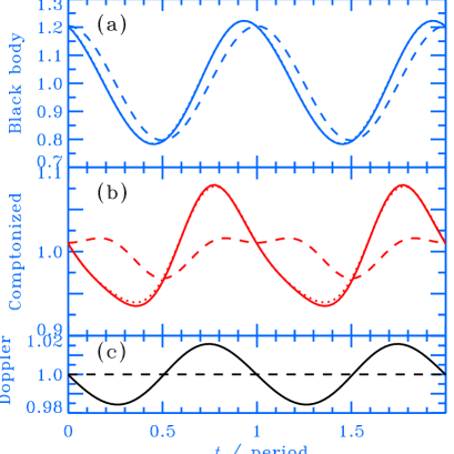
Figure 4: The bolometric black body and Comptonized fluxes, and the Doppler factor $\delta$ as functions of phase. Dashed curves correspond to a slowly rotating neutron star. Solid curves give the profiles modified by the Doppler boosting and aberration for a neutron star of rotational frequency 401 Hz. (Other parameters are given in Fig. 5.) Light bending in the Schwarzschild geometry is accounted for. Dotted curves (coinciding completely with the solid one at the upper panel) show the results of multiplication of the dashed curves by $\delta^{5}$ and $\delta^{4}$ for the black body and the Comptonized emission, respectively (see eqs [3.3] and [17]).

Neglecting the Doppler effect and using equation (3.3) one can relate the variability amplitude of the black body flux to the angles $i$ and $\theta$ and the neutron star radius (Beloborodov 2002):

$$A\equiv(F_{\max}-F_{\min})/(F_{\max}+F_{\min})=U/Q,$$ (19)

where we defined

$$U = (1-r_{g}/R)\sin i\ \sin\theta,$$

$$Q = r_{g}/R+(1-r_{g}/R)\cos i\ \cos\theta.$$ (20)

This peak-to-peak amplitude is $\sqrt{2}$ larger than sometimes quoted rms amplitude if the light curve is a pure sine wave.

For a circular spot of an angular radius $\rho$ emitting as a black body, the observed flux can be obtained from equation (3.3):

$$F_{\rho}=\left(1-\frac{r_{g}}{R}\right)^{2}\frac{I_{0}}{D^{2}}\pi R^{2}\sin^{2}\rho\left(Q+\frac{r_{g}}{R}\tan^{2}\frac{\rho}{2}+U\cos\phi\right),$$ (21)

if the spot is always visible, i.e. $\cos(i+\theta+\rho)>\mu_{v}$. Here the intensity is related to the local temperature $I_{0}=\sigma_{\rm SB}T_{0}^{4}/\pi$. We can easily now obtain the oscillation amplitude:

$$A_{\rho}=\frac{U}{\displaystyle Q+\frac{r_{g}}{R}\tan^{2}\frac{\rho}{2}}.$$ (22)

Equation (21) allows us to estimate the size of the spot $R\rho$ from the equation:

$$r_{\rm spot,\infty}^{2}=R^{2}\sin^{2}\rho\left(Q+\frac{r_{g}}{R}\tan^{2}\frac{\rho}{2}\right),$$ (23)

if the distance $D$, the temperature $T_{\infty}=T_{0}(1-r_{g}/R)^{1/2}$ and the observed phase-averaged black body flux $\overline{F_{\rho}}=\sigma_{\rm SB}T_{\infty}^{4}r_{\rm spot,\infty}^{2}/D^{2}$ (and thus $r_{\rm spot,\infty}$) are known from observations. For small $\rho$, the spot radius is $R\rho=r_{\rm spot,\infty}Q^{-1/2}$.

4 Results

We fit the observed pulse profiles in the energy bands 3–4 keV and 12–18 keV simultaneously. The second band is completely dominated by the Comptonized radiation and thus gives direct information about its angular distribution. In the lower energy band, the black body affects the observed pulse profile. Since the mass of the compact star in SAX J1808.4$-$3658  is not known, we consider masses between $M=1.0{\rm M_{\odot}}$ and $1.6{\rm M_{\odot}}$. Masses in the range of $1.4$–$1.6{\rm M_{\odot}}$ are expected for neutron stars in low mass X-ray binaries that have accreted material from their binary companions, lower masses are possible, for example, for strange stars. We restrict the inclination to $i<82\degr$ to be consistent with the absence of the X-ray eclipses (Bildsten & Chakrabarty 2001). The best-fitting parameters are presented in Table LABEL:table:fit. The two sets of errors correspond to the 90 and 99 per cent confidence intervals with $\Delta\chi^{2}=2.71$ and $6.63$, respectively.

Table 1: Best-fitting parameters

$M$	$R$	$R/r_{g}$	$i$	$\theta$	$\tau$	$\tau_{\rm es}$ or $a$	$\chi^{2}/$dof
(${\rm M_{\odot}}$)	(km)		(deg)	(deg)
Model 1:           Electron scattering slab, $I^{\rm sc}(\mu)\propto I_{\infty}(\tau_{\rm es},\mu)$
$1.0$	$5.15^{+0.25}_{-0.15}\ {}^{+0.45}_{-0.35}$	$1.72^{+0.08}_{-0.05}\ {}^{+0.15}_{-0.12}$	$74^{+8}_{-20}\ {}^{+8}_{-24}$	$20^{+6}_{-2.5}\ {}^{+10}_{-3.5}$	$0.08^{+0.07}_{-0.04}\ {}^{+0.09}_{-0.05}$	$0.84^{+0.22}_{-0.16}\ {}^{+0.28}_{-0.19}$	$29.7/26$
$1.2$	$7.0^{+0.5}_{-0.4}\ {}^{+1.1}_{-0.6}$	$1.94^{+0.14}_{-0.11}\ {}^{+0.31}_{-0.17}$	$82^{+0}_{-5}\ {}^{+0}_{-18}$	$13^{+1.5}_{-1}\ {}^{+3}_{-1.5}$	$0.06^{+0.04}_{-0.02}\ {}^{+0.08}_{-0.03}$	$0.59^{+0.09}_{-0.06}\ {}^{+0.24}_{-0.10}$	$35.3/26$
$1.4$	$8.8^{+2.9}_{-0.4}\ {}^{+4.5}_{-0.7}$	$2.1^{+0.7}_{-0.1}\ {}^{+1.1}_{-0.17}$	$82^{+0}_{-5}\ {}^{+0}_{-8}$	$11^{+0.5}_{-3}\ {}^{+1}_{-4}$	$0.08^{+0.03}_{-0.06}\ {}^{+0.05}_{-0.07}$	$0.52^{+0.05}_{-0.21}\ {}^{+0.12}_{-0.22}$	$47.3/26$
$1.6$	$13.4^{+0.8}_{-1.0}\ {}^{+1.6}_{-1.7}$	$2.8^{+0.17}_{-0.21}\ {}^{+0.33}_{-0.35}$	$82^{+0}_{-1}\ {}^{+0}_{-2}$	$7^{+1}_{-0.5}\ {}^{+1.5}_{-1}$	$0.05^{+0.02}_{-0.01}\ {}^{+0.03}_{-0.01}$	$0.33^{+0.04}_{-0.03}\ {}^{+0.07}_{-0.03}$	$61.4/26$
Model 2:           $I^{\rm sc}(\mu)\propto 1+a\mu$
$1.0$	$5.0^{+0.2}_{-0.1}\ {}^{+0.4}_{-0.2}$	$1.67^{+0.07}_{-0.03}\ {}^{+0.13}_{-0.07}$	$82^{+0}_{-25}\ {}^{+0}_{-32}$	$19^{+6}_{-1}\ {}^{+11}_{-2}$	$0.09^{+0.07}_{-0.01}\ {}^{+0.09}_{-0.01}$	$-0.69^{+0.10}_{-0.02}\ {}^{+0.12}_{-0.03}$	$28.1/26$
$1.2$	$6.4^{+0.3}_{-0.2}\ {}^{+0.8}_{-0.3}$	$1.78^{+0.08}_{-0.05}\ {}^{+0.22}_{-0.08}$	$82^{+0}_{-8}\ {}^{+0}_{-17}$	$14^{+1.5}_{-0.5}\ {}^{+3}_{-1}$	$0.14^{+0.03}_{-0.02}\ {}^{+0.06}_{-0.03}$	$-0.74^{+0.06}_{-0.02}\ {}^{+0.10}_{-0.04}$	$32.2/26$
$1.4$	$8.3^{+0.6}_{-0.4}\ {}^{+1.6}_{-0.7}$	$1.97^{+0.15}_{-0.09}\ {}^{+0.39}_{-0.16}$	$82^{+0}_{-5}\ {}^{+0}_{-13}$	$11^{+1}_{-1}\ {}^{+1.5}_{-1.5}$	$0.14^{+0.03}_{-0.01}\ {}^{+0.04}_{-0.02}$	$-0.80^{+0.04}_{-0.04}\ {}^{+0.08}_{-0.07}$	$38.7/26$
$1.6$	$10.8^{+0.6}_{-0.8}\ {}^{+2.6}_{-0.9}$	$2.25^{+0.13}_{-0.17}\ {}^{+0.47}_{-0.27}$	$82^{+0}_{-3}\ {}^{+0}_{-7}$	$8.5^{+1.0}_{-0.5}\ {}^{+1.5}_{-1}$	$0.15^{+0.02}_{-0.01}\ {}^{+0.04}_{-0.01}$	$-0.89^{+0.05}_{-0.01}\ {}^{+0.08}_{-0.01}$	$44.8/26$

We see from Table LABEL:table:fit that the results obtained with the two models 1 and 2 are very consistent with each other. For both models, a large inclination is preferred and the lower limit is $i>65\degr$ (at 99 per cent confidence level) for $M\gtrsim 1.2{\rm M_{\odot}}$. The fits become much worse at masses higher than $1.6{\rm M_{\odot}}$. The estimated stellar radius (even in $r_{g}$ units) grows with the mass and varies between $\sim 1.7r_{g}$ and $\sim 2.3r_{g}$ ($\sim 2.8r_{g}$ for model 1). Using simple analytical estimations we explain the physical reasons behind this behaviour in § 5.1. The radii are consistent with some of the neutron star equations of state if $M\gtrsim 1.4{\rm M_{\odot}}$. For a smaller assumed mass of $1.2{\rm M_{\odot}}$, the radius is more consistent with the equations of state for strange stars, while for even smaller mass of $1{\rm M_{\odot}}$, the obtained stellar radius of $R\sim 5$ km is too small even for a strange star (see § 5.2 and Fig. 7 for details).

The colatitude $\theta$ of the spot centre varies approximately as $\propto R^{-1}$. A larger $\theta$ is needed for smaller $R$ in order to keep the spot velocity (and thus the Doppler factor) at approximately constant level.

The estimated radius of the spot (not a fitting parameter) corrected for orientation and gravitational effects varies between 3.0 and 3.7 km for $M=1.0{\rm M_{\odot}}$ and $1.6{\rm M_{\odot}}$, respectively. One can get some estimates of the size of the Comptonizing region from a rather large difference between the best-fitting $\tau_{\rm es}$ and $\tau$ obtained in model 1. The values of $\tau_{\rm es}$ are consistent with the optical depths obtained from the fits of the time-averaged spectrum with a Comptonization model for a slab geometry. For example, model compps (Poutanen & Svensson 1996), gives $\tau_{\rm es}=0.5$ for the electron temperature $kT_{e}=90$ keV (which is not well constrained because of the low signal above 100 keV). This leads us to a conclusion that a large fraction of the black body photons reaches the observer without interaction with the hot Comptonizing medium (contradicting assumed homogeneous slab geometry). In order to get the “effective” $\tau\sim 0.1$ (see eq. [14]), about 40 per cent of the black body area should be covered by the Comptonizing medium with $\tau_{\rm es}\sim 0.5$, while the remaining 60 per cent should emit as a pure black body (i.e. with no $\exp(-\tau/\mu)$ reduction due to scattering). Thus, we conclude that the radius of the Comptonizing region $r_{\rm spot,c}$ is about 2 km.

The angular distributions of the scattered radiation (see dashed curve in Fig. 5b) determined by parameters $\tau_{\rm es}$ and $a$ is also very similar for models 1 and 2. Model 2 is somewhat less restrictive and therefore gives generally better fits. The required emission pattern is certainly very much different from that given by the Lambert law and more radiation is escaping at intermediate angles $\alpha^{\prime}\sim 50\degr$ than along the normal. It is this pattern which is responsible for the origin of a strong first harmonic (i.e. at double spin frequency) in the pulsar light curve at high energies (modified also by Doppler effects, see Fig. 4 and § 3.3).

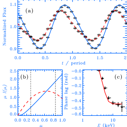
Figure 5: (a) Observed normalized pulse profiles in the energy bands 3–4 keV (circles) and 12–18 keV (squares) and the best-fitting model light curves (solid and dashed curves) as a function of pulsar phase (two periods are plotted, zero phase is chosen when a spot is closest to the observer). A neutron star with the mass $M=1.4{\rm M_{\odot}}$ and the radius $R=2r_{g}=8.4$ km and inclination $i=80\degr$ are assumed. The best-fitting parameters (model 2) are $\theta=11\degr$, $\tau=0.16$, $a=-0.78$ and $\chi^{2}$/dof$=40.1/28$. (b) The angular distribution of the intrinsic black body (solid curve) and Comptonized (dashed curve) fluxes $\mu I(\mu)$ (here $\mu=\cos\alpha^{\prime}$) in the co-rotating frame normalized as $\int\mu I(\mu)d\mu=1$. Only the range of angles between the dotted lines is actually observed. (c) The observed (crosses) and the model (solid curve) phase lags at the pulsar frequency relative to the 3–4 keV band.

In order to check the dependence of the results on the assumed geometry, we repeated the fitting procedure considering an extreme case with a point-like Comptonizing source at the centre of the black body spot. The best-fitting parameters are similar to the situation where both emitting regions coincide. This is expected since the size of the emission region should not play a large role since $r_{\rm spot}=R\rho<R$. However, when estimating the size of the spot, we assumed the soft emission is a black body, i.e. the observed color temperature is equal to the effective temperature. For the hydrogen and helium atmospheres of weakly magnetized neutron stars one expects that the color correction is $f_{\rm col}\equiv T_{\rm col}/T_{\rm eff}=1.6$–$1.8$ (Zavlin, Pavlov & Shibanov 1996). The shift of the peak of the emission towards higher energies from the corresponding black body emission results from the fact that the outer layers of the atmosphere are cooler than the deeper layers. Since the bound-free and free-free cross-sections rapidly decrease with increasing photon energy, one sees deeper and hotter layers at high energies. However, when the accretion takes place and the radiative shock forms (its existence is supported by the presence of the hard X-ray tail), the soft radiation can be produced by reprocessing the hard photons from the shock. The temperature gradient of the atmosphere then can be opposite to that of standard neutron star atmospheres. Now the hot layers are at the top, softer photons are coming from the hotter region (since absorption cross-section is large for small energies), while hard photons are coming from the cooler region below and the color correction can be smaller than unity. The actual vertical temperature dependence is however unknown.

To investigate the influence of different possible color corrections on our best-fitting parameters, we consider two extreme cases of $f_{\rm col}=1.5$ and $0.7$ and fitted the data with model 2. The area of the “black body” spot now changes by a factor $f_{\rm col}^{2}$. For $f_{\rm col}=1.5$, the spot centre colatitude $\theta$ increases by about 20 per cent comparing to the case of no color correction. Since now the spot is larger, $\theta$ has to increase to keep the same oscillation amplitude (see eq. [22]). The best-fitting stellar radius increases significantly only for the smallest considered mass of $M=1{\rm M_{\odot}}$ reaching $5.5$ km, for $M=1.2{\rm M_{\odot}}$ the radius is $6.7$ km, while for higher masses the change is negligible. In the case of $f_{\rm col}=0.7$ the spot becomes smaller and $\theta$ also slightly decreases. At $M=1{\rm M_{\odot}}$ the best-fitting radius is now $4.8$ km, while all other parameters remain the same within the errors. There is no change in the best-fitting parameters for higher stellar masses. This results from the fact that the light curve depends weakly on the spot size if it small comparing to the stellar radius (see eqs [21, 22]).

One of the important assumptions that can affect our results is that the two emission components are assumed to be co-spatial or are at least co-centred. In our interpretation the Comptonized emission peaks earlier than the black body due to a different angular distribution more affected by the Doppler effect. However, an additional phase shift is possible if the Comptonized emission region is physically shifted on the stellar surface. We fitted the data with model 2 and the phase shift $\Delta\phi$ of the Comptonized emission as an additional free parameter. A major effect of adding a new parameter is that the confidence interval for the stellar radius increases. Thus, for example, for $M=1.4{\rm M_{\odot}}$, the best fit with $\chi^{2}$/dof$=34/25$ was obtained for $\Delta\phi=0.1$ rad (a positive shift corresponds to an earlier arrival time) and other parameters very similar to those presented in Table LABEL:table:fit, while the constraints on the radius weaken: $R=8.8^{+4.2}_{-0.7}$ (90 per cent confidence limits). An $F$-test gives $F=3.5$ which corresponds to a 7 per cent chance that the decrease in $\chi^{2}$ was random (i.e. the improvement is not highly statistically significant).

We show one of the fits to the pulse profiles with the fixed $M$, $i$, and $R$ in Fig. 5a. The corresponding intrinsic angular distribution of the radiation flux in the two spectral components is shown in Fig. 5b. One sees a dramatic difference between the dependences of the black body and Comptonized components. The observed energy dependence of the pulse profiles and the phase lags at the pulsar frequency between different energies (Fig. 5c) are reproduced reasonably well. A natural consequence of the model is that the phase lags change significantly at smaller energies together with the black body contribution to the total flux, while they reach a constant value at about 6–8 keV where the black body flux becomes negligible (see also Gierliński et al. 2002). Since in reality the angular dependence of Comptonization radiation is a function of energy, one would expect a weaker dependence of lags on energy even above 10 keV.

5 Discussion

5.1 Constraints from the oscillation amplitude and the Doppler factor

         

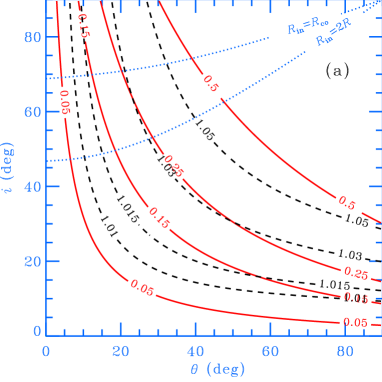
Figure 6: (a) Contours of the constant variability amplitude $A$ given by equation (19) (solid curves) and the contours of constant maximum Doppler factor $\delta_{\max}$ (dashed curves) for a black body spot ($\nu=401$ Hz, $M=1.4{\rm M_{\odot}}$ and $R=2r_{g}=8.4$ km). The dotted curves define the $i-\theta$ relation where the photon trajectories from the antipodal spot (that without the disc would reach the observer) cross the disc at the minimum distance of $2R$ and the corotation radius $R_{\rm co}$. These curves are computed using approximate photon trajectories from Beloborodov (2002). The inner disc radius smaller than $2R$ (or $R_{\rm co}$) would block the antipodal spot from the observer in the area above the corresponding curve.
(b) Contours of the constant variability amplitude $A=0.18$ (solid curves) computed using equation (19) for different stellar radii measured in $r_{g}$ units and the interception points of these curves with the contours of constant $\delta_{\max}=1.015$ for different stellar masses: $M=1.0{\rm M_{\odot}}$ (squares), $1.2{\rm M_{\odot}}$ (triangles), $1.4{\rm M_{\odot}}$ (circles), and $1.6{\rm M_{\odot}}$ (diamonds).

Let us consider first for simplicity the black body emission from a single spot. In that case, the Doppler effect does not change significantly the light curve (compare dashed and solid curve in Fig. 4a) and thus it is mainly characterized by the amplitude $A$ that can be estimated for a slowly rotating star using equation (19). For a given $R/r_{g}$, the amplitude in its turn depends on $i$ and $\theta$ only. Thus, at the $i-\theta$ plane we can determine a curve that would correspond to a given amplitude $A$ (see solid curves in Fig. 6a). One notes that this curve is symmetric around the $i=\theta$ line since one can exchange $i$ and $\theta$ in the expression for $A$ (see eqs [19–3.3]) without affecting the result. If the black body emission is more beamed towards the spot normal because of a non-zero $\tau$, this curve will be somewhat shifted down and left since $A$ then increases. For example, the black body variability amplitude observed in SAX J1808.4$-$3658 is $\sim 25$ per cent (Gierliński et al. 2002) and, correcting for $\tau$, we can determine the region at the $i-\theta$ plane where it can be reproduced for a given $R/r_{g}$.

The situation is different when we consider a less beamed emission pattern $I(\alpha)\propto 1+a\cos\alpha$ with $a<0$ (i.e. in our case radiation above $\sim 8$ keV). The oscillation amplitude is then strongly affected by the Doppler effect (compare dashed and solid curve in Fig. 4b). The maximum of the Doppler factor and the spot projected area are shifted in phase by $\sim$ 0.25 of the period and the peak of the emission is then shifted towards the phase where $\delta$ has the maximum. However, the amplitude and the shape of the profile carry the information needed to determine $a$ and the maximum Doppler factor $\delta_{\max}$. Again at the $i-\theta$ plane we can determine the curve of constant $\delta_{\max}$ (see dashed curves in Fig. 6a). Note, that since the Doppler factor (to the first order in $\beta$) depends on the product $\sin i\sin\theta$ (see eqs [9–11]), but not on $i$ and $\theta$ individually, this curve is almost symmetric around the $i=\theta$ line.

A very important point here is that the curves of constant $A$ and $\delta_{\max}$ do not coincide (see Fig. 6a). At the $i-\theta$ plane thus there are at most two points (for a given star mass $M$ and radius $R$) with the given values of these two parameters: points of the crossing of the curves of constant $A$ and $\delta_{\max}$. This leaves some ambiguity regarding the exchange of $i$ and $\theta$. It is possible, however, that the number of crossing points is one or even zero which would then mean that there is no physical solution with a given Doppler factor and the variability amplitude within the considered model.

Let us now apply our simple arguments to the data on SAX J1808.4$-$3658. The observed light curve implies a maximum Doppler factor about 1.015 and the variability amplitude $A$ for a black body spot given by equation (19) of $\sim 0.18$ (actually observed higher value results from a sharper emission pattern with $\tau\sim 0.1$, see eq. [14]). The contours of constant $A$ do not depend on the stellar mass but only on the radius measured in $r_{g}$ (see Fig. 6b). We can now find a point at the $i-\theta$ plane that satisfy both constraints. The curves of the constant $A$ and $\delta_{\max}$ intercept in two points: at a large inclination and small $\theta$ as well as at a small inclination $i\lesssim 20\degr$ and large $\theta$.

The second solution is much less probable. First, we do not see any emission from the secondary antipodal spot. This implies that either it is blocked by the star itself (which in turn requires the stellar radius to be $\gtrsim 4r_{g}$ for $i\sim 15\degr$ and $\theta\sim 60\degr$), or it is blocked by the accretion disc. In the later case we have additional constraints. At inclinations smaller than $\sim 50\degr$ an upper limit on the inner disc radius (i.e. the magnetospheric radius) required to block the secondary spot is $R_{\rm in}\lesssim 2R$ (see lower dotted curve in Fig. 6a). With such a small inner radius, the expected amplitude of Compton reflection component should be probably larger than the observed $\Omega/2\pi\sim 0.1$ (unless the inner disc is highly ionised) and the shock should appear at uncomfortably large angle from the rotational pole if the magnetic field is a central dipole. On the other hand, at inclinations $i\gtrsim 70\degr$ the antipodal spot is blocked by the disc if the magnetospheric radius is smaller than the corotation radius $R_{\rm co}=31(M/1.4{\rm M_{\odot}})^{1/3}(P/2.5{\rm ms})^{2/3}$ km which is also required for accretion to take place. Second, small $i$ is inconsistent with the X-ray (Chakrabarty & Morgan 1998) and optical (Giles, Hill & Greenhill 1999; Homer et al. 2001) modulations at the binary period, and finally, it is also inconsistent with the lower limit $i>28\degr$ obtained by Wang et al. (2001) based on the modelling of the optical/IR emission with the X-ray irradiated disc. We conclude that large inclinations $i>50\degr$ and small $\theta\sim 5\degr$–$20\degr$ are preferred to small $i$ and large $\theta$.

For small stellar masses $M=1.0{\rm M_{\odot}}$, the interception point for given $A$ and $\delta_{\max}$ fixes the possible inclination $i$ between $55\degr$ and $80\degr$ depending on the assumed radius. The minimum possible radius still satisfying constraints on the inclination angle $i<82\degr$ is $R=1.8r_{g}$. For higher masses, the minimum possible radius (in $r_{g}$ units) increases, reaching $R=2.5r_{g}$ for $M=1.4{\rm M_{\odot}}$, and for $M=1.6{\rm M_{\odot}}$ there is no solution whatsoever. Thus it is quite natural that the $\chi^{2}$ is worse for the high mass star (see Table LABEL:table:fit). This simple analysis also explains why the higher is the stellar mass, the higher the inclination should be in order to satisfy constraints on both $A$ and $\delta_{\max}$.

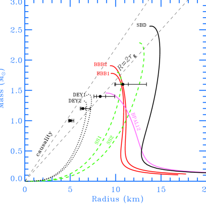
Figure 7: Constraints on the radius of the compact star depending on the assumed mass are shown by circles with double error bars (for 90 and 99 per cent confidence intervals) for the fits with model 2. For comparison we show also the relations between the compact star mass and its radius for several equations of state of neutron stars and strange stars. The labels for neutron star equations of state are BBB1 and BBB2 – Baldo, Bombaci & Burgio (1997), BPAL12 – Prakash et al. (1997), SBD – Sahu, Basu & Datta (1993), while for the strange stars SS1 and SS2 correspond to the MIT bag model (see Gondek-Rosińska, Kluźniak & Stergioulas 2003 for details) and DEY1 and DEY2 to the equation of state of Dey et al. (1998) computed as in Gondek-Rosińska et al. (2000). All realistic equations of state lie to the right of the causality line. The line $R=2r_{g}$ is shown to guide the eye.

5.2 Stellar masses and radii

Our results (see Table LABEL:table:fit and Fig. 7) put constraints on mass of the compact object. For $M=1{\rm M_{\odot}}$ the obtained stellar radius of $R\sim 5$ km is too small to be consistent with any existing equations of state for neutron or strange stars. For masses higher than $1.6{\rm M_{\odot}}$, the fits are much worse than for smaller masses. Thus we conclude that the stellar mass is bound between 1.2 and 1.6 solar masses.

We can also put constraints on the equations of state of compact stars (which of course could be much stronger if the mass of compact object were known). Thus, if $M=1.2{\rm M_{\odot}}$ the only possible solution is a strange star (Chakrabarty 1991; Li et al. 1999; Ray et al. 2000; Gondek-Rosińska et al. 2000) with the equation of state derived by Dey et al. (1998). For the mass about $1.4{\rm M_{\odot}}$, almost all known neutron star equations of state predict larger radii than our best-fitting value. The exception are the models similar to BPAL12 from Prakash et al. (1997) and the models with a kaon condensate (Glendenning & Schaffner-Bielich 1999; see Lattimer & Prakash 2001 for more details). However, the maximum mass for these models is $\sim 1.5{\rm M_{\odot}}$ which is smaller than the best estimate of the neutron star mass in Vela X-1 of $1.86\pm 0.16{\rm M_{\odot}}$ (Barziv et al. 2001). Thus we are inclined to conclude that our constraints together with the minimum neutron star mass in Vela X-1 put a lower limit on to the neutron star mass in SAX J1808.4$-$3658 of about $1.5{\rm M_{\odot}}$. Strange stars (MIT bag models) with maximum masses in the range of $1.5$–$1.7{\rm M_{\odot}}$ would also fit into our constraints. At larger mass of $M=1.6{\rm M_{\odot}}$ a strange star is still a possible solution as well as a neutron star described by equations of state similar to that of Baldo et al. (1997), while the most stiff equations of state, such as for example that by Sahu et al. (1993), can be ruled out (see Fig. 7).

Assuming alignment of the orbital angular momentum and that of the compact object, we can estimate the mass of the companion star $M_{c}$ from our lower limits on the inclination of the rotational axis (see Table LABEL:table:fit). Using the measured mass function $f_{x}=(M_{c}\sin\ i)^{3}/(M+M_{c})^{2}=3.78\times 10^{-5}{\rm M_{\odot}}$ (Chakrabarty & Morgan 1998) we find that $M_{c}=0.041\pm 0.002,0.0445\pm 0.0015,0.0478\pm 0.0005{\rm M_{\odot}}$ for $M=1.2,1.4,1.6{\rm M_{\odot}}$, respectively. The companion radius is about $0.13R_{\odot}$ (Bildsten & Chakrabarty 2001).

The mass measurements of radio pulsars in binary systems and their neutron star companions revealed their very narrow distribution with the mean $M\sim 1.35{\rm M_{\odot}}$ and a very small dispersion (Thorsett & Chakrabarty 1999). No evidence for extensive mass accretion was found. In order to spin up a star with the moment of inertia $\sim 10^{45}$ g cm² to the frequency of 400 Hz one needs to accrete just about $\Delta M\approx 0.1{\rm M_{\odot}}$. Thus if the initial mass is within the same distribution one does not expect the mass of the compact object to exceed $1.5$–$1.6{\rm M_{\odot}}$. For a mass of $1.4{\rm M_{\odot}}$, our best-fitting radius (with model 2) is $R=8.3^{+0.6}_{-0.4}$ km (90 per cent confidence interval). Such a radius is consistent with the upper limit $R<7.5(M/{\rm M_{\odot}})^{1/3}$ km obtained from the fact that pulsations are observed at fluxes differing by a factor of 100 (Burderi & King 1998; Li et al. 1999). Here one assumes that the magnetic and the ram pressure from the accreting material are equal at the magnetospheric radius which is larger than the stellar radius $R$ and smaller than the corotation radius $R_{\rm co}$. For $M=1.5{\rm M_{\odot}}$, our best fit $R=9.5\pm 0.5$ km is already inconsistent with the given upper limit. This constraint, however, is more relaxed if the magnetic field does not have a dipole structure and/or the accretion disc is not gas-pressure dominated (Psaltis & Chakrabarty 1999).

5.3 Emission mechanism

The angular dependence of the hard radiation that is needed to produce the observed pulse profiles above 8 keV is consistent with that expected from the electron scattering dominated slab with Thomson optical depth $\tau_{\rm es}\sim 0.3$–$1$. It would be natural to assume that the emission originates in a plane-parallel shock at the surface of the compact star (Basko & Sunyaev 1976). The observed spectral slope $\Gamma\sim 2$ (the energy spectrum $E^{-1}$) is expected from bulk motion Comptonization in a radiation dominated strong shock (Blandford & Payne 1981). Most of the papers on this subject neglect generation of new soft photons by reprocessing the hard radiation at the neutron star surface which would significantly soften the emergent spectra. Thus, in order to reproduce $\Gamma\sim 2$ slope, thermal Comptonization should play an important role (Lyubarskii & Sunyaev 1982). As discussed in Gilfanov et al. (1998), there should exist a mechanism that adjust the spectrum so that it does not change much when the accretion rate varies by a factor of 100. Reprocessing of the hard photons produced in a shocked region into soft ones that cool the shock could be such a mechanism. This two-phase structure in the energy balance is known to stabilize the spectrum at the observed values when the optical depth is of the order of unity (Haardt & Maraschi 1993; Stern et al. 1995). The electron temperature adjusts itself to the variations of the optical depth (and luminosity) so that the product of the electron temperature and optical depth is approximately constant.

Variation of the accretion rate that is the main candidate for the aperiodic variability observed in SAX J1808.4$-$3658 (Wijnands & van der Klis 1998b) thus can cause the changes in the optical depth, but not in the spectral shape. However, the relative amplitude of the black body and Comptonized components can vary. Indeed, at small luminosities the black body seems to the more prominent (Gilfanov et al. 1998) which would correspond to a smaller optical depth of the Comptonizing layer. A larger relative normalization of the black body component should result also in a higher variability amplitude which in fact was increasing from 4 to 7 per cent (rms amplitude) over the duration of the 1998 April outburst (Cui et al. 1998).

There could be additional effects related to the electron-positron pair production (by photon-photon interactions) which becomes important when the compactness parameter $l=L\sigma_{T}/(r_{\rm spot,c}\ m_{e}c^{3})$ is larger than unity. For the luminosity of $L\sim 3\times 10^{36}$ erg s^-1 (which is a characteristic luminosity during the April 1998 outburst of SAX J1808.4$-$3658, see Gierliński et al. 2002) and the emission region size of $r_{\rm spot,c}=2$ km, the compactness is about $400$ and it could be much larger if the region has a smaller height. Thus, the data are consistent with the presence of pairs which could be responsible for producing the optical depth in the range $\tau_{\rm es}\sim 0.3-1$ depending on the compactness and for fixing the electron temperature in the range $50-100$ keV working as a thermostat (Stern et al. 1995; Poutanen & Svensson 1996; Malzac, Beloborodov & Poutanen 2001). If the hard radiation is slightly beamed towards the neutron star surface due to the bulk motion, the amount of soft photons produced would be larger than from an isotropic source and there will be no problem in reproducing the observed spectrum that satisfies the energy balance (cf. Gierliński et al. 2002).

The radiation escaping from the shock can be affected by cold plasma in the accretion column. Assuming the area of the emission region of $\pi r_{\rm spot,c}^{2}\sim 12$ km² and the accretion rate $\dot{M}=2\times 10^{16}$ g s^-1 (needed to produce the observed luminosity at efficiency of 0.15) one can estimate from the continuity equation the characteristic optical depth of the plasma over the distance equal to the spot radius $\tau=n_{e}\sigma_{T}r_{\rm spot,c}\approx 0.8$. (At higher distances from the star, the magnetic field lines diverge and photons can escape freely.) This means that the flow can affect the radiation escaping along the normal to the spot and the radiation can be blocked from the observer at certain phases. Since the area emitting the black body radiation is larger than the cross-section of the accretion column, one would expect that the effect of shadowing is smaller for the black body. Possibly, this effect is observed in the light curve where the hard radiation has a break at $\phi=0$ (see Fig. 5a). We may also see this effect from the best-fitting angular distribution (see Fig. 5b) which shows a drop along the normal at $\mu=\cos\alpha^{\prime}\sim 1$.

5.4 Origin of soft lags

Our results confirm the proposal by Gierliński et al. (2002) that the main physical reason behind the soft lags is a two-component nature of the spectrum. A natural consequence of this model is a break in the phase lag at the energy where the black body component vanishes, i.e. around 8 keV (see Fig. 5c). We showed here that the black body and the Comptonized components having different angular distribution generate light curves which are affected by the Doppler effect in a different way. The Doppler shift is an important ingredient but not the major cause of the soft lags. In our model, the Doppler effect comes into play only through its influence on the variability amplitude of the bolometric flux.

On the other hand, Ford (2000) and Weinberg et al. (2001) proposed a model where the lags in SAX J1808.4$-$3658 are produced by the Doppler effect alone through its influence on the monochromatic flux. In both papers a black body emission from the spot is assumed. When the spot is moving towards the observer, the Doppler effect shift the spectrum towards higher energies, while motions away from the observer softens the spectrum and generate a deficit at high energies. Thus, higher energy photons, in the tail of the black body distribution, arrive only at phases when motion is predominantly towards the observer, while the flux of photons at the peak of the black body distribution has a maximum together with the projected area, i.e. quarter of the period later. This results in hard leads (or soft lags) as well. As discussed in Gierliński et al. (2002), there are a number of problems with this proposal. First, the photons in the black body tail contribute very little to the total observed spectrum above 8 keV which is dominated by the hard Comptonized component. Thus, any soft lags in the black body flux would be completely invisible in the total flux. Second, a break in the phase lag energy dependence does not have any physical explanation in that model.

Even stronger Doppler boosting is expected when photons from the spot are scattered off a much more rapidly rotating inner disc (Sazonov & Sunyaev 2001). The scattered radiation will be leading or lagging the incident spot radiation depending on whether the disc is co-rotating or counter-rotating. For a black body radiation from the spot, this would translate into soft lags or leads, respectively. However, since the spectrum from the spot is closer to a power law, no phase lags should appear (Chen & Shaham 1989). A different angular distribution of the black body and Comptonized components as well as a non-coherent nature of scattering can affect this result. It could be an interesting problem for future studies. We believe that this model is not directly related to SAX J1808.4$-$3658, since the spot is probably situated close to the rotational pole and the fraction of the spot photons scattered in the disc is negligibly small.

Cui et al. (1998) interpreted soft lags as due to Compton down-scattering of intrinsic hard photons with energies above 10 keV in a cold electron cloud of Thomson optical depth $\tau_{\rm es}\sim 10$. The softer photons (scattered more times) escape from the medium later producing soft lags. As the authors pointed out, the hard photons should escape to the observer directly through some kind of a hole in the cloud since otherwise a spectral cutoff should appear at $\sim 511/\tau_{\rm es}^{2}\sim 5$ keV (e.g. Sunyaev & Titarchuk 1980; Lightman, Lamb & Rybicki 1981). This model, however, predicts a significantly reduced variability in the softer energy band (Chang & Kylafis 1983; Brainerd & Lamb 1987) contrary to what is observed.

6 Summary

The two main spectral components, black body and Comptonized, are clearly identified in the time-averaged spectrum of SAX J1808.4$-$3658. The pulse profiles show significant energy dependence and the softer photons lag the harder ones. Such a behaviour can be reproduced if the hard Comptonized emission peaks earlier than the black body emission (Gierliński et al. 2002). The black body component shows about 25 per cent (peak-to-peak) variability amplitude and the Doppler effect (producing a $\sim$ 7 per cent variability) does not change its pulse profile much (Fig. 4). The Comptonized emission from an optically thin slab with a broader (“fan”–like) angular distribution has an intrinsically smaller variability amplitude. The Doppler effect then shifts significantly the peak of the pulse producing soft lags.

By modelling the observed pulse profiles, we obtained an upper limit on the mass of the compact object $M\lesssim 1.6{\rm M_{\odot}}$. We also put the lower limit of $M\gtrsim 1.2{\rm M_{\odot}}$ on the stellar mass since for smaller masses the obtained radii are too small to be consistent with any published equation of state for neutron or strange stars. This also constrains the inclination of the system to be larger than $65\degr$. For the masses $1.4{\rm M_{\odot}}<M<1.6{\rm M_{\odot}}$, the best-fitting stellar radii $R=8$–$11$ km are consistent with those given by the neutron star equations of states as well as some strange star models, while for $M\sim 1.2{\rm M_{\odot}}$ with that given by the equations of state for strange stars only.

References

- [\citeauthoryearBaldo et al.1997] Baldo M., Bombaci I., Burgio G. F., 1997, A&A, 328, 274
- [\citeauthoryearBarziv et al.2001] Barziv O., Kaper L., Van Kerkwijk M. H., Telting J. H., Van Paradijs J., 2001 A&A, 377, 925
- [\citeauthoryearBasko & Sunyaev1976] Basko M. M., Sunyaev R. A., 1976, MNRAS, 175, 395
- [\citeauthoryearBeloborodov2002] Beloborodov A. M., 2002, ApJ, 566, L85
- [\citeauthoryearBildsten & Chakrabarty2001] Bildsten L., Chakrabarty D., 2001, ApJ, 557, 292
- [\citeauthoryearBlandford & Payne1981] Blandford R., Payne D., 1981, MNRAS, 194, 1033
- [\citeauthoryearBrainerd & Lamb1987] Brainerd J., Lamb F. K., 1987, ApJ, 317, L33
- [\citeauthoryearBurderi & King1998] Burderi L., King A., 1998, ApJ, 505, L135
- [\citeauthoryearChakrabarty & Morgan1998] Chakrabarty D., Morgan E. H., 1998, Nature, 394, 346
- [\citeauthoryearChakrabarty1991] Chakrabarty S., 1991, Phys. Rev. D, 43, 627
- [\citeauthoryearChang & Kylafis1983] Chang K. M., Kylafis N. D., 1983, ApJ, 265, 1005
- [\citeauthoryearChen & Shaham1989] Chen K., Shaham J., 1989, ApJ, 339, 279
- [\citeauthoryearCui et al.1998] Cui W., Morgan E. H., Titarchuk L. G., 1998, ApJ, 504, L27
- [\citeauthoryearDey1998] Dey M., Bombaci I., Dey J., Ray S., Samanta B. C., 1998, Phys. Lett. B, 438, 123
- [\citeauthoryearFord2000] Ford E. C., 2000, ApJ, 535, L119
- [\citeauthoryearGalloway et al.2002] Galloway D. K., Chakrabarty D., Morgan E. H., Remillard R. A., 2002, ApJ, 576, L137
- [\citeauthoryearGhisellini1999] Ghisellini G., 1999, in Casciaro B., Fortunato D., Francaviglia M. & Masiello A., eds, XIII National Meeting on General Relativity of the SIGRAV, Recent developments in General Relativity. Springer-Verlag (astro-ph/9905181)
- [\citeauthoryearGierliński et al.2002] Gierliński M., Done C., Barret D., 2002, MNRAS, 331, 141
- [\citeauthoryearGiles, Hill & Greenhill1999] Giles A. B., Hill K. M., Greenhill J. G., 1999, MNRAS, 304, 47
- [\citeauthoryearGilfanov et al.1998] Gilfanov M., Revnivtsev M., Sunyaev R., Churazov E., 1998, A&A, 338, L83
- [\citeauthoryearGlendenning & Schaffner-Bielich1999] Glendenning N. K., Schaffner-Bielich J., 1999, Phys. Rev. C, 60, 025803
- [\citeauthoryearGondek-Rosińska et al.2000] Gondek-Rosińska D., Bulik T., Zdunik L., Gourgoulhon E., Ray S., Dey J., Dey M., 2000, A&A, 363, 1005
- [\citeauthoryearGondek-Rosińska et al.2003] Gondek-Rosińska D., Kluźniak W., Stergioulas N., 2003, A&A, submitted (astro-ph/0206470)
- [\citeauthoryearHaardt & Maraschi1993] Haardt F., Maraschi L., 1993, ApJ, 413, 507
- [\citeauthoryearHomer et al.2001] Homer L., Charles P. A., Chakrabarty D., van Zyl L., 2001, MNRAS, 325, 1471
- [\citeauthoryearin ’t Zand et al.2001] in ’t Zand J. J. M. et al., 2001, A&A, 372, 916
- [\citeauthoryearLattimer & Prakash2001] Lattimer J. M., Prakash M., 2001, ApJ, 550, 426
- [\citeauthoryearLi1999] Li X. D., Bombaci I., Dey M., Dey J., van der Heuvel E. P. J., 1999, Phys. Rev. Lett., 83, 3776
- [\citeauthoryearLightman et al.1981] Lightman A. P., Lamb D. Q., Rybicki G. B., 1981, ApJ, 166, 301
- [\citeauthoryearLightman et al.1975] Lightman A. P., Press W. H., Price R. H., Teukolsky S. A., 1975, Problem book in relativity and gravitation. Princeton University Press, Princeton
- [\citeauthoryearLind & Blandford1985] Lind K. R., Blandford R. D., 1985, ApJ, 295, 358
- [\citeauthoryearLyubarskii & Sunyaev1982] Lyubarskii Yu. E., Sunyaev R. A., 1982, SvA Lett., 8, 330
- [\citeauthoryearNath et al.2002] Nath N. R., Strohmayer T. E., Swank J. H., 2002, ApJ, 564, 353
- [\citeauthoryearMalzac, Beloborodov & Poutanen2001] Malzac J., Beloborodov A. M., Poutanen J., 2001, MNRAS, 326, 417
- [\citeauthoryearMarkwardt et al.2002] Markwardt C. B., Swank J. H., Strohmayer T. E., in ’t Zand J. J. M., Marshall F. E., 2002, ApJ, 575, L21
- [\citeauthoryearMarkwardt et al.2003] Markwardt C. B., Smith E., Swank J. H., 2003, IAU Circ. 8080
- [\citeauthoryearMiller & Lamb1998] Miller M. C., Lamb F. K., 1998, ApJ, 499, L37
- [\citeauthoryearMisner et al.1973] Misner C. W., Thorn K. S., Wheeler J. A., 1973, Gravitation. Freeman, San Francisco
- [\citeauthoryearMuno et al.2002] Muno M. P., Özel F., Chakrabarty D., 2002, ApJ, 581, 550
- [\citeauthoryearPechenick et al.1983] Pechenick K. R., Ftaclas C., Cohen J. M., 1983, ApJ, 274, 846
- [\citeauthoryearPoutanen & Svensson1996] Poutanen J., Svensson R., 1996, ApJ, 470, 249
- [\citeauthoryearPrakash et al.1997] Prakash M., Bombaci I., Prakash M., Ellis P. J., Lattimer J. M., Knorren R., 1997, Phys. Rep., 280, 1
- [\citeauthoryearPsaltis & Chakrabarty1999] Psaltis D., Chakrabarty D., 1999, ApJ, 521, 332
- [\citeauthoryearPsaltis et al.2000] Psaltis D., Özel F., DeDeo S., 2000, ApJ, 544, 390
- [\citeauthoryearRay et al.2000] Ray S., Dey J., Dey M., Ray K., Samanta B. C., 2000, A&A, 364, L89
- [\citeauthoryearSahu et al.1993] Sahu P. K., Basu R., Datta B., 1993, ApJ, 416, 267
- [\citeauthoryearSazonov & Sunyaev2001] Sazonov S. Y., Sunyaev R. A., 2001, A&A, 373, 241
- [\citeauthoryearStern et al.1995] Stern B. E., Poutanen J., Svensson R., Sikora M., Begelman M. C., 1995, ApJ, 449, L13
- [\citeauthoryearStrohmayer et al.1997] Strohmayer T. E., Jahoda K., Giles A. B., Lee U., 1997, ApJ, 486, 355
- [\citeauthoryearStrohmayer & Bildsten2003] Strohmayer T., Bildsten L., 2003, in Lewin W. H. G, van der Klis M., eds, Compact Stellar X-Ray Sources. Cambridge University Press, Cambridge, in press (astro-ph/0301544)
- [\citeauthoryearSunyaev & Titarchuk1980] Sunyaev R. A., Titarchuk L. G., 1980, A&A, 86, 121
- [\citeauthoryearSunyaev & Titarchuk1985] Sunyaev R. A., Titarchuk L. G., 1985, A&A, 143, 374
- [\citeauthoryearTerrell1959] Terrell J., 1959, Phys. Rev., 116, 1041
- [\citeauthoryearThorsett & Chakrabarty1999] Thorsett S. E., Chakrabarty D., 1999, ApJ, 512, 288
- [\citeauthoryearWang et al.2001] Wang Z. et al., 2001, ApJ, 563, L61
- [\citeauthoryearWeinberg et al.2001] Weinberg N., Miller M. C., Lamb D. Q., 2001, ApJ, 546, 1098
- [\citeauthoryearWijnands & van der Klis1998a] Wijnands R., van der Klis M., 1998a, Nature, 394, 344
- [\citeauthoryearWijnands & van der Klis1998b] Wijnands R., van der Klis M., 1998b, ApJ, 507, L63
- [\citeauthoryearZavlin et al.1996] Zavlin V. E., Pavlov G. G., Shibanov Yu. A., 1996, A&A, 315, 141
- [\citeauthoryearZdziarski et al.1996] Zdziarski A. A., Johnson W. N., Magdziarz P., 1996, MNRAS, 283, 193