Transfer of energy and angular momentum in magnetic coupling process

Abstract

The transfer of energy and angular momentum in the magnetic coupling (MC) of a rotating black hole (BH) with its surrounding accretion disc is discussed based on a mapping relation derived by considering the conservation of magnetic flux with two basic assumptions: (i)the magnetic field on the horizon is constant, (ii) the magnetic field on the disc surface varies as a power law with the radial coordinate of the disc. The following results are obtained: (i) the transfer direction of energy and angular momentum between the BH and the disc depends on the position of a co-rotation radius relative to the MC region on the disc, which is eventually determined by the BH spin; (ii) the evolution characteristics of a rotating BH in the MC process without disc accretion are depicted in a parameter space, and a series of values of the BH spin are given to indicate the evolution characteristics; (iii) the efficiency of converting accreted mass into radiation energy of a BH-disc system is discussed by considering coexistence of disc accretion and the MC process; (iv) the MC effects on disc radiation and emissivity index are discussed and it is concluded that they are consistent with the recent XMM-Newton observation of the nearby bright Seyfert 1 galaxy MCG-6-30-15 with reference to a variety of parameters of the BH-disc system.

1 INTRODUCTION

Recently, the magnetic coupling of a rotating black hole (BH) with its surrounding disc has been investigated by certain authors (Blandford 1999; Li 2000, Li 2002a, b, hereafter Li02a and Li02b, respectively; Li & Paczynski 2000; Wang, Xiao & Lei 2002, hereafter WXL). This coupling can be regarded a variation of the Blandford-Znajek (BZ) process, proposed two decades ago (Blandford & Znajek 1977). With closed magnetic field lines connecting a rotating BH with the disc, energy and angular momentum can be transferred from the BH to the disc and henceforth this energy mechanism is referred to as the magnetic coupling (MC) process. The load in the MC process is the surrounding disc, which is much better understood than the remote astrophysical load in the BZ process. Energy and angular momentum are always transferred from the BH to the unknown remote load in the BZ process, while the transfer direction of energy and angular momentum in the MC process depends not only on the angular velocity of the BH but also on that of the disc where each closed field line penetrates.

Usually, the transfer of energy and angular momentum in the MC process is stated as follows: ’If a BH rotates faster than its surrounding disc, it exerts a torque on the disc and energy and angular momentum are extracted from the BH and transferred to the disc, and vice versa’. However, this statement is rather vague and only applicable to the case that the closed magnetic field lines are attached to the inner edge of the disc. In a more realistic model the closed field lines are assumed to connect the BH horizon with the disc by attaching a ring with inner and outer boundary as shown in Fig.1, where $r_{in}$ and $r_{out}$ are the radii of the inner and outer boundary of the MC region, respectively, and $\theta_{1}$ and $\theta_{2}$ are the corresponding angular coordinates on the BH horizon.

Figure 1: The poloidal magnetic field connecting a rotating BH with its surrounding disc

It is shown in WXL that the width of the MC region should not be given at random, which can be determined by conservation of magnetic flux in the context of general relativity. In this paper the mapping relation derived in WXL between the angular coordinate on the BH horizon and the radial coordinate on the disc is modified by a boundary condition on the closed field lines connecting the two loops in the equatorial plane of the BH. It turns out that the transfer direction of energy and angular momentum is determined by the position of the co-rotation radius relative to the MC region, and ultimately depends on the BH spin eventually. In addition, other MC effects, such as BH entropy change, efficiency of releasing energy, disc radiation and emissivity, also appear to be related intimately to the BH spin . In particular, as argued in Li02b, the MC effects on emissivity are consistent with the recent XMM-Newton observation of the nearby bright Seyfert 1 galaxy MCG-6-30-15. We find that a variety of MC parameters are suitable for the above observation.

This paper is organized as follows. In Section 2 we give the basic evolution equation of a BH in MC process, and derive a modified mapping relation between the angular coordinate on the BH horizon and the radial coordinate on the disc. In Section 3 the evolution characteristics of a rotating BH in the MC process without disc accretion are depicted in terms of the BH spin in a parameter space, and a series of values of the BH spin are given to indicate the evolution features. The sequence of these values are related to the transfer of energy and angular momentum between the BH and the disc, and guaranteed by the second law of BH thermodynamics (Wald 1984). In Section 4 the efficiency of BH-disc systems in converting accreted mass into radiation energy is discussed in terms of the coexistence of disc accretion and the MC process. In addition, we discuss MC effects on disc radiation and emissivity index that are consistent with the recent XMM-Newton observation of the nearby bright Seyfert 1 galaxy MCG-6-30-15. Finally in Section 5, we summarize our main results.

In order to facilitate the discussion of the correlation of BH spin with MC effects in an analytic way, we make the following assumptions:

(i) The disc is both stable and perfectly conducting, and the closed magnetic field lines are frozen in the disc.

(ii) The disc is thin and Keplerian, and lies in the equatorial plane of the BH with the inner boundary being at the marginally stable orbit.

(iii) The magnetic field is assumed to be weak, and the effect of instabilities of the disc and the magnetic field are ignored; The magnetosphere is stationary, axisymmetric and force-free outside the BH and the disc;.

(iv) The magnetic field is assumed to be constant on the horizon, and to vary as a power law with the radial coordinate of the disc.

Throughout this paper the geometric units $G=c=1$ are used.

2 BASIC EQUATIONS FOR BH EVOLUTION AND MAPPING RELATION IN THE MC PROCESS

As argued by Macdonald & Thorne (1982, hereafter MT), the magnetic field on the horizon is brought and held by the surrounding magnetized disc. So both disc accretion and the MC process should be taken into account in our model for BH evolution. Based on conservation of energy and angular momentum, the basic equations for BH evolution with the coexistence of disc accretion and the MC process are written as

$${dM}\mathord{\left/{\vphantom{{dM}{dt}}}\right.\kern-1.2pt}{dt}=E_{ms}\dot{M}_{D}-P_{MC},$$ (1)

$${dJ}\mathord{\left/{\vphantom{{dJ}{dt}}}\right.\kern-1.2pt}{dt}=L_{ms}\dot{M}_{D}-T_{MC}.$$ (2)

Combining equations (1) and (2) we have the evolution of BH spin:

$$\begin{array}[]{l}da_{*}/dt=M^{-2}({L_{ms}\dot{M}_{D}-T_{MC}})\\ \\ \quad\quad\quad\quad-2M^{-1}a_{*}({E_{ms}\dot{M}_{D}-P_{MC}}).\end{array}$$ (3)

Now we give a brief explanation for the quantities in equations (1) and (2). $M$ and $J$ are mass and angular momentum of the BH, respectively. $a_{*}\equiv J\mathord{\left/{\vphantom{J{M^{2}}}}\right.\kern-1.2pt}{M^{2}}$ is the dimensionless angular momentum of the BH, and referred to as the BH spin. $E_{ms}$ and $L_{ms}$ are specific energy and angular momentum corresponding to the inner edge of the thin disc, i.e. the last stable circular orbit, respectively (Novikov & Thorne 1973). $\dot{M}_{D}$ is the accretion rate. At first sight, $\dot{M}_{D}$ will be affected by the MC process owing to angular momentum transferred between the rotating BH and the disc. We derived the MC correction on $\dot{M}_{D}$ by considering the conservation law of angular momentum and the angular momentum transferred at the inner edge of the disc (see Appendix A in WXL). Unfortunately, the modification to $\dot{M}_{D}$, equation (42) in WXL, is incorrect, since accretion rate cannot depend on radius in a stationary flow, and the validity of the following results of sections 5 and 6 in WXL is doubtful. In this paper the MC effects on the accretion rate are not considered for the following reasons.

(i) A constant accretion rate is required by the conservation of mass in a stationary disc.

(ii) From equations (61) and (62) we find that the viscous torque related to disc radiation can regulates itself everywhere to counteract the effects of angular momentum transferred into the disc on the accretion rate.

In the basic evolution equations (1) and (2), $P_{MC}$ and $T_{MC}$ are the rates of extracting energy and angular momentum from the rotating BH by the MC process, and henceforth are referred to as the MC power and the MC torque, respectively. We have derived the expressions for $P_{MC}$ and $T_{MC}$ in WXL as follows:

$${P_{MC}}\mathord{\left/{\vphantom{{P_{MC}}{P_{0}}}}\right.\kern-1.2pt}{P_{0}}=2a_{*}^{2}\int_{\theta_{1}}^{\pi\mathord{\left/{\vphantom{\pi 2}}\right.\kern-1.2pt}2}{\frac{\beta\left({1-\beta}\right)\sin^{3}\theta d\theta}{2-\left({1-q}\right)\sin^{2}\theta}},$$ (4)

$${T_{MC}}\mathord{\left/{\vphantom{{T_{MC}}{T_{0}}}}\right.\kern-1.2pt}{T_{0}}=4a_{*}\left({1+q}\right)\int_{\theta_{1}}^{\pi\mathord{\left/{\vphantom{\pi 2}}\right.\kern-1.2pt}2}{\frac{\left({1-\beta}\right)\sin^{3}\theta d\theta}{2-\left({1-q}\right)\sin^{2}\theta}},$$ (5)

where $\theta$ is the angular coordinate on the horizon varying from $\theta_{1}$ to $\pi\mathord{\left/{\vphantom{\pi 2}}\right.\kern-1.2pt}2$. $P_{0}$ and $T_{0}$ are defined as

$$\left\{{\begin{array}[]{l}P_{0}=\left\langle{B_{H}^{2}}\right\rangle M^{2}\approx B_{4}^{2}M_{8}^{2}\times 6.59\times 10^{44}erg\cdot s^{-1},\\ T_{0}=\left\langle{B_{H}^{2}}\right\rangle M^{3}\approx B_{4}^{2}M_{8}^{3}\times 3.26\times 10^{47}g\cdot cm^{2}\cdot s^{-2},\\ \end{array}}\right.$$ (6)

and $B_{4}$ and $M_{8}$ are $\sqrt{\left\langle{B_{H}^{2}}\right\rangle}$ and $M$ in the units of $10^{4}gauss$ and $10^{8}M_{\odot}$, respectively. The parameter $\beta\equiv{\Omega_{D}}\mathord{\left/{\vphantom{{\Omega_{D}}{\Omega_{H}}}}\right.\kern-1.2pt}{\Omega_{H}}$ is defined as the ratio of the angular velocity on the thin disc to that on the horizon, and we have the following expressions:

$$\Omega_{H}=a_{*}/(2r_{{}_{H}}),\quad\quad r_{{}_{H}}=M(1+q),\quad\quad q=\sqrt{1-a_{*}^{2}},\\$$ (7)

and

$$\Omega_{F}=\Omega_{D}=\frac{1}{M(\chi^{3}+a_{*})},\\$$ (8)

where $r_{{}_{H}}$ is the radius of the horizon of a Kerr BH. $\Omega_{F}$ is the angular velocity of the closed field line connecting the BH and the disc, and $\Omega_{F}=\Omega_{D}$ arises from the freezing-in condition in the disc (MT).

In order to calculate $P_{MC}$ and $T_{MC}$ we should first determine the mapping relation between the BH horizon and the disc. Considering the flux tube consisting of two adjacent magnetic surfaces “$i$” and “$i+1$” as shown in Fig.1, we have $\Delta\Psi_{H}=\Delta\Psi_{D}$ required by continuum of magnetic flux, i.e.

$$B_{\bot}2\pi\left({\varpi\rho}\right)_{r=r_{{}_{H}}}d\theta=-B_{z}2\pi\left({{\varpi\rho}\mathord{\left/{\vphantom{{\varpi\rho}{\sqrt{\Delta}}}}\right.\kern-1.2pt}{\sqrt{\Delta}}}\right)_{\theta=\pi\mathord{\left/{\vphantom{\pi 2}}\right.\kern-1.2pt}2}dr,$$ (9)

where $B_{\bot}$ and $B_{z}$ are the normal components of magnetic field at the horizon and the disc, respectively, and

$$\left({\varpi\rho}\right)_{r=r_{{}_{H}}}=\left({\Sigma\sin\theta}\right)_{r=r_{{}_{H}}}=2Mr_{{}_{H}}\sin\theta,$$ (10)

$$\left({{\varpi\rho}\mathord{\left/{\vphantom{{\varpi\rho}{\sqrt{\Delta}}}}\right.\kern-1.2pt}{\sqrt{\Delta}}}\right)_{\theta=\pi\mathord{\left/{\vphantom{\pi 2}}\right.\kern-1.2pt}2}=\Sigma\mathord{\left/{\vphantom{\Sigma{\sqrt{\Delta}}}}\right.\kern-1.2pt}{\sqrt{\Delta}}=\alpha^{-1}\rho,$$ (11)

where

$$\alpha=\left({{\rho\sqrt{\Delta}}\mathord{\left/{\vphantom{{\rho\sqrt{\Delta}}\Sigma}}\right.\kern-1.2pt}\Sigma}\right)_{\theta=\pi\mathord{\left/{\vphantom{\pi 2}}\right.\kern-1.2pt}2}=\sqrt{\frac{1-2\chi_{ms}^{-2}\xi^{-1}+a_{*}^{2}\chi_{ms}^{-4}\xi^{-2}}{1+a_{*}^{2}\chi_{ms}^{-4}\xi^{-2}+2a_{*}^{2}\chi_{ms}^{-6}\xi^{-3}}}.$$ (12)

In equation (12) $\xi\equiv r\mathord{\left/{\vphantom{r{r_{ms}}}}\right.\kern-1.2pt}{r_{ms}}$is a dimensionless radial parameter defined in terms of the radius $r_{ms}$ of the last stable circular orbit. Following Blandford (1976) we assume that $B_{z}$ varies as

$$B_{z}\propto\xi^{-n}.$$ (13)

Table 1. Some quantities related to $a_{*}^{eq}$

n	$a_{*}^{eq}$	$\xi_{out}\left({a_{*}^{eq}}\right)$	$\xi_{c}\left({a_{*}^{eq}}\right)$	$R_{\xi}$	$R_{P}$	$R_{T}$
1.1	0.2924	1.28273	1.10957	0.63274	-1.26867	-1.0104
1.5	0.2908	1.29863	1.11273	0.60636	-1.28244	-1.0107
3.0	0.2835	1.38780	1.12758	0.49025	-1.35549	-1.0123

Owing to the lack of knowledge of configuration of the magnetic field in the gap region between the horizon and the inner edge of the disc, we proposed the following assumptions in WXL: (a) the inner boundary of the MC region is located at the inner edge of the disc, with which the closed field lines connect the horizon at $\theta=\pi\mathord{\left/{\vphantom{\pi 2}}\right.\kern-1.2pt}2$; (b) the strength of the magnetic field at the horizon is equal to that at the inner edge of the disc. However the former is probably greater than the latter by numerical simulation in the disc (Ghosh & Abramowicz 1997, and the references therein). Considering conservation of magnetic flux in the inner boundary of the MC region, we propose the following relation to replace assumption (b):

$$2\pi r_{{}_{H}}B_{\bot}=2\pi\varpi_{D}\left({r_{ms}}\right)B_{z}\left({r_{ms}}\right),$$ (14)

where $\varpi_{D}\left({r_{ms}}\right)$ is the cylindrical radius at the inner edge of a thin disc and reads

$$\varpi_{D}\left({r_{ms}}\right)=M\chi_{ms}^{2}\sqrt{1+\chi_{ms}^{-4}a_{*}^{2}+2\chi_{ms}^{-6}a_{*}^{2}}.$$ (15)

Equation (14) implies conservation of magnetic flux corresponding to the two loops of the same infinitesimal width, and the ratio of $B_{\bot}$ to $B_{z}\left({r_{ms}}\right)$ varies from 1.8 to 3 for $0<a_{*}<1$. Incorporating equations (13) and (14) we have

$$B_{z}=B_{\bot}\left[{{r_{{}_{H}}}\mathord{\left/{\vphantom{{r_{{}_{H}}}{\varpi_{D}\left({r_{in}}\right)}}}\right.\kern-1.2pt}{\varpi_{D}\left({r_{in}}\right)}}\right]\xi^{-n}.$$ (16)

Combining equations (10)—(16) into equation (9) we have

$$\sin\theta d\theta=-\mbox{G}\left({a_{*};\xi,n}\right)d\xi,$$ (17)

where

$$\begin{array}[]{l}G({a_{*};\xi,n})\\ \\ =\frac{\xi^{1-n}\chi_{ms}^{2}\sqrt{1+a_{*}^{2}\chi_{ms}^{-4}\xi^{-2}+2a_{*}^{2}\chi_{ms}^{-6}\xi^{-3}}}{2\sqrt{\left({1+a_{*}^{2}\chi_{ms}^{-4}+2a_{*}^{2}\chi_{ms}^{-6}}\right)\left({1-2\chi_{ms}^{-2}\xi^{-1}+a_{*}^{2}\chi_{ms}^{-4}\xi^{-2}}\right)}}.\end{array}$$ (18)

Integrating equation (17) and setting $\xi=\xi_{in}=1$ at $\theta=\pi\mathord{\left/{\vphantom{\pi 2}}\right.\kern-1.2pt}2$, we express the mapping relation by

$$\cos\theta=\int_{1}^{\xi}{\mbox{G}\left({a_{*};\xi,n}\right)}d\xi,$$ (19)

and the outer boundary $\xi_{out}\equiv{r_{out}}\mathord{\left/{\vphantom{{r_{out}}{r_{ms}}}}\right.\kern-1.2pt}{r_{ms}}$ of the MC region can be determined by the following equation:

$$\cos\theta_{1}=\int_{1}^{\xi_{out}}{\mbox{G}\left({a_{*};\xi,n}\right)}d\xi.$$ (20)

From equation (20) we find that $\xi_{out}\left({a_{*};n,\theta_{1}}\right)$ behaves as a non-monotonic function of $a_{*}$ for the given $n$ and $\theta_{1}$ as shown in Fig.2. It is noted that $\theta_{1}$ is taken as $\pi\mathord{\left/{\vphantom{\pi 6}}\right.\kern-1.2pt}6$ throughout this paper except where indicated otherwise.

Figure 2: The curves of $\xi_{c}$(dot-dashed line) and $\xi_{out}$ versus $a_{*}$ for $0<a_{*}<1$ with $n=1.1,\mbox{ 1.5}$ and $3.0$ in solid, dashed and dotted lines, respectively.

The co-rotation radius $r_{c}$ is defined as the radius on the disc where the angular velocity $\Omega_{D}$ of the disc is equal to the BH angular velocity $\Omega_{H}$, i.e.

$${\Omega_{D}}\mathord{\left/{\vphantom{{\Omega_{D}}{\Omega_{H}}}}\right.\kern-1.2pt}{\Omega_{H}}=\frac{2\left({1+q}\right)}{a_{*}}\left[{\left({\sqrt{\xi}\chi_{ms}}\right)^{3}+a_{*}}\right]^{-1}=1.$$ (21)

From equation (21) we can express $r_{c}$ in terms of a parameter $\xi_{c}={r_{c}}\mathord{\left/{\vphantom{{r_{c}}{r_{ms}}}}\right.\kern-1.2pt}{r_{ms}}$ as follows:

$$\xi_{c}\left({a_{*}}\right)={r_{c}}\mathord{\left/{\vphantom{{r_{c}}{r_{ms}}}}\right.\kern-1.2pt}{r_{ms}}=\chi_{ms}^{-2}\left({1-q}\right)^{-1/3}\left({1+q}\right).$$ (22)

The parameter $\xi_{c}$ decreases monotonically with $a_{*}$ is shown by the dot-dashed line in Fig. 2, where there exist two kinds of intersections: one is that the curve $\xi_{c}\left({a_{*}}\right)$ intersects with each curve of $\xi_{out}\left(a_{*};\theta_{1},n\right)$, which is indicated by $(a_{*}^{out},\xi_{out}^{{}^{\prime}})$; the other is that it intersects with $\xi_{in}=1$, which is indicated by $\left({0.3594,\mbox{ }1}\right)$. These intersections imply that the co-rotation radius $r_{c}$ is located at the outer and inner boundaries of the MC region for $a_{*}=a_{*}^{out}$ and $a_{*}^{in}=0.3594$, respectively. The MC region is divided into two parts by $\xi_{c}$: the inner MC region (henceforth IMCR) for $1<\xi<\xi_{c}$ and the outer MC region (henceforth OMCR) for $\xi_{c}<\xi<\xi_{out}$. Therefore energy and angular momentum are always transferred by the closed magnetic field lines from the BH into the OMCR with $\Omega_{D}<\Omega_{H}$, while the transfer direction reverses for IMCR with $\Omega_{D}>\Omega_{H}$. The correlation of the BH spin with the transfer direction is given as follows:

(i) For $0.3594<a_{*}<1$ we have $\xi_{c}$ within the inner edge, and the MC region is simply the OMCR with the transfer direction from the BH to the disc;

(ii) For $a_{*}^{out}<a_{*}<0.3594$ we have $1<\xi_{c}<\xi_{out}$, and the transfer direction is from the BH to the disc in the OMCR, while it is from disc in the IMCR to the BH;

(iii) For $0\leq a_{*}<a_{*}^{out}$ we have $\xi_{c}>\xi_{out}$, and the MC region is simply the IMCR with the transfer direction from the disc to the BH.

3 BH EVOLUTION IN THE MC PROCESS WITHOUT DISC ACCRETION

3.1 Equilibrium spin of a BH in MC process without disc accretion

In order to highlight the MC effects on BH evolution we discuss a specific case where disc accretion is absent. In this case a rotating BH can attain its equilibrium spin $a_{*}^{eq}$ in the MC process for $1<\xi_{c}<\xi_{out}$. The basic evolution equations (1), (2) and (3) become

$${dM}\mathord{\left/{\vphantom{{dM}{dt}}}\right.\kern-1.2pt}{dt}=-P_{MC},$$ (23)

$${dJ}\mathord{\left/{\vphantom{{dJ}{dt}}}\right.\kern-1.2pt}{dt}=-T_{MC},$$ (24)

$${da_{*}}\mathord{\left/{\vphantom{{da_{*}}{dt}}}\right.\kern-1.2pt}{dt}=-M^{-2}T_{MC}+2M^{-1}a_{*}P_{MC}.$$ (25)

Setting ${da_{*}}\mathord{\left/{\vphantom{{da_{*}}{dt}}}\right.\kern-1.2pt}{dt}=0$, we have

$$T_{MC}=2Ma_{*}P_{MC}.$$ (26)

Substituting equations (4), (5) and (19) into equation (26), we can obtain $a_{*}^{eq}$ for the given parameters $\theta_{1}$ and $n$ by resolving the following equation:

$$\int_{1}^{\xi_{out}}{\frac{\left({1-\beta}\right)\left({1-\beta+\beta q}\right)}{2\csc^{2}\theta-\left({1-q}\right)}}G\left({a_{*};\xi,n}\right)d\xi=0.$$ (27)

In order to discuss the transportation of energy and angular momentum at $a_{*}^{eq}$, we define the following ratios:

$$R_{P}={P_{MC}^{in}}\mathord{\left/{\vphantom{{P_{MC}^{in}}{P_{MC}^{out}}}}\right.\kern-1.2pt}{P_{MC}^{out}},\quad R_{T}={T_{MC}^{in}}\mathord{\left/{\vphantom{{T_{MC}^{in}}{T_{MC}^{out}}}}\right.\kern-1.2pt}{T_{MC}^{out}},$$ (28)

where $P_{MC}^{in}$ and $T_{MC}^{in}$ are the rates of transferring energy and angular momentum in the IMCR, respectively, and $P_{MC}^{out}$ and $T_{MC}^{out}$ are the rates of transferring energy and angular momentum in OMCR, respectively. By using the mapping relation (19) these quantities can be expressed as follows:

$$P_{MC}^{in}=2a_{*}^{2}P_{0}\int_{1}^{\xi_{c}}{\frac{\beta\left({1-\beta}\right)G\left({a_{*};\xi,n}\right)}{2\csc^{2}\theta-\left({1-q}\right)}}d\xi,$$ (29)

$$P_{MC}^{out}=2a_{*}^{2}P_{0}\int_{\xi_{c}}^{\xi_{out}}{\frac{\beta\left({1-\beta}\right)G\left({a_{*};\xi,n}\right)}{2\csc^{2}\theta-\left({1-q}\right)}}d\xi,$$ (30)

$$T_{MC}^{in}=4a_{*}T_{0}\left({1+q}\right)\int_{1}^{\xi_{c}}{\frac{\left({1-\beta}\right)G\left({a_{*};\xi,n}\right)}{2\csc^{2}\theta-\left({1-q}\right)}}d\xi,$$ (31)

$$T_{MC}^{out}=4a_{*}T_{0}\left({1+q}\right)\int_{\xi_{c}}^{\xi_{out}}{\frac{\left({1-\beta}\right)G\left({a_{*};\xi,n}\right)}{2\csc^{2}\theta-\left({1-q}\right)}}d\xi.$$ (32)

From equations (19), (22), (27)—(32) we obtain some quantities related to $a_{*}^{eq}$ as listed in Table 1.

From Table 1 we obtain the following results:

(i) Both $R_{P}$ and $R_{T}$ are less than $-1$, and these imply

$$\begin{array}[]{l}P_{MC}\left({a_{*}^{eq}}\right)=P_{MC}^{in}\left({a_{*}^{eq}}\right)+P_{MC}^{out}\left({a_{*}^{eq}}\right)<0,\\ \\ T_{MC}\left({a_{*}^{eq}}\right)=T_{MC}^{in}\left({a_{*}^{eq}}\right)+T_{MC}^{out}\left({a_{*}^{eq}}\right)<0,\end{array}$$ (33)

which means that the transportation of energy and angular momentum in OMCR is dominated by that in IMCR, i.e. they are transferred as a whole from the disc to the BH at equilibrium spin $a_{*}^{eq}$.

(ii) Defining $R_{\xi}\equiv{\left({\xi_{c}-1}\right)}\mathord{\left/{\vphantom{{\left({\xi_{c}-1}\right)}{\left({\xi_{out}-\xi_{c}}\right)}}}\right.\kern-1.2pt}{\left({\xi_{out}-\xi_{c}}\right)}$ to indicate the ratio of the radial width of IMCR to that of OMCR, we find that both $R_{\xi}$ and $a_{*}^{eq}$ decrease as the increasing $n$, while both $\xi_{out}\left({a_{*}^{eq}}\right)$ and $\xi_{c}\left({a_{*}^{eq}}\right)$ increase with increasing $n$. These results are related to the conservation of magnetic flux with the fact that more magnetic field is concentrated in IMCR for greater value of $n$.

3.2 BH evolution in the MC process without disc accretion

We can discuss the BH evolution in the corresponding parameter space as proposed in WXL. Evolution equations (23), (24) and (25) can be rewritten as

$$\left\{{\begin{array}[]{l}{dM}/{dt}=-P_{MC}=2P_{0}f\left({a_{*};n,\theta_{1}}\right),\\ \\ f\left({a_{*};n,\theta_{1}}\right)=-a_{*}^{2}\int_{1}^{\xi_{out}}{\frac{\beta\left({1-\beta}\right)G\left({a_{*};\xi,n}\right)}{2\csc^{2}\theta-\left({1-q}\right)}}d\xi,\\ \end{array}}\right.$$ (34)

$$\left\{{\begin{array}[]{l}{dJ}\mathord{\left/{\vphantom{{dJ}{dt}}}\right.\kern-1.2pt}{dt}=-T_{MC}=4T_{0}h\left({a_{*};n,\theta_{1}}\right),\\ \\ h\left({a_{*};n,\theta_{1}}\right)=-a_{*}\left({1+q}\right)\int_{1}^{\xi_{out}}{\frac{\left({1-\beta}\right)G\left({a_{*};\xi,n}\right)}{2\csc^{2}\theta-\left({1-q}\right)}}d\xi,\\ \end{array}}\right.$$ (35)

$$\left\{{\begin{array}[]{l}{da_{*}}\mathord{\left/{\vphantom{{da_{*}}{dt}}}\right.\kern-1.2pt}{dt}=4T_{0}M^{-2}g\left({a_{*};n,\theta_{1}}\right),\\ \\ g\left({a_{*};n,\theta_{1}}\right)=-a_{*}\left({1+q}\right)\times\\ \quad\quad\quad\quad\quad\quad\quad\quad\int_{1}^{\xi_{out}}{\frac{\left({1-\beta}\right)\left({1-\beta+\beta q}\right)G\left({a_{*};\xi,n}\right)}{2\csc^{2}\theta-\left({1-q}\right)}}d\xi.\\ \end{array}}\right.$$ (36)

From equations (34)—(36), we find that $f\left({a_{*};n,\theta_{1}}\right)$, $h\left({a_{*};n,\theta_{1}}\right)$ and $g\left({a_{*};n,\theta_{1}}\right)$ have the same signs as those of ${dM}\mathord{\left/{\vphantom{{dM}{dt}}}\right.\kern-1.2pt}{dt}$, ${dJ}\mathord{\left/{\vphantom{{dJ}{dt}}}\right.\kern-1.2pt}{dt}$ and ${da_{*}}\mathord{\left/{\vphantom{{da_{*}}{dt}}}\right.\kern-1.2pt}{dt}$, respectively. Setting $f\left({a_{*};n,\theta_{1}}\right)=0$, $h\left({a_{*};n,\theta_{1}}\right)=0$ and $g\left({a_{*};n,\theta_{1}}\right)=0$ for $\theta_{1}=\pi\mathord{\left/{\vphantom{\pi 6}}\right.\kern-1.2pt}6$, we have three characteristic curves in the two-dimension space consisting of the parameters $a_{*}$ and $n$ as shown in Fig. 3, where each black dot with an arrowhead represents one BH evolution state. From left to right, the parameter space is divided into four regions by these three curves, and the signs of the rates of change of $M$, $J$ and $a_{*}$ in these four regions are listed in Table 2.

Figure 3: Parameter space for BH evolution in the MC process with

$1.1\leq n\leq 2.1$ and $\mbox{0.}2881<a_{*}<0.2960$.

Table 2. The signs of $dM/dt$, $dJ/dt$, and $da_{*}/dt$

       in the regions of parameter space

Region	Position	$da_{*}/dt$	$dJ/dt$	$dM/dt$
I	left of $g=0$	$>0$	$>0$	$>0$
II	between $g=0$ and $h=0$	$<0$	$>0$	$>0$
III	between $h=0$ and $f=0$	$<0$	$<0$	$>0$
IV	right of $f=0$	$<0$	$<0$	$<0$

From Fig.3 we find that $P_{MC}$ changes its sign from negative to positive at $a_{*}^{P}$ ($f=0)$ and $T_{MC}$ does it at $a_{*}^{T}$ ($h=0)$. The inequality, $a_{*}^{T}<a_{*}^{P}$, holds for all possible values of $n$, because the curve $h=0$ is located on the left of $f=0$ as shown in Fig.3. This result means that $P_{MC}$ is negative with the positive $T_{MC}$ in the value range $a_{*}^{T}<a_{*}<a_{*}^{P}$. However, it does not mean that the transfer direction of energy is opposite to that of angular momentum in the IMCR or in the OMCR. In fact, as argued above, the transfer direction of energy is always the same as that of angular momentum either in the IMCR or in the OMCR, and the opposite signs of $P_{MC}$ and $T_{MC}$ rest in the fact that $P_{MC}^{out}$ and $T_{MC}^{in}$ are dominated by $P_{MC}^{in}$ and $T_{MC}^{out}$ for the above value range of the BH spin, respectively. We can explain this order of the BH spin by using the second law of BH thermodynamics in the next section. The order of the above specific values of BH spin is given as follows:

$$0<a_{*}^{out}<a_{*}^{eq}<a_{*}^{T}<a_{*}^{P}<a_{*}^{in}<1.$$ (37)

We can use the parameter space to determine the evolution characteristics of a rotating BH in the MC process, provided that the initial BH spin $a_{*}$ and the power law index $n$ are given. For example a BH with initial spin $a_{*}^{P}<a_{*}<1$ will evolve to $a_{*}^{eq}$ and reach the curve $g=0$ eventually by passing region IV, III and II one after another. So we can determine its evolution characteristics in each evolution stage represented by the corresponding region in Fig.3.

The status of MC region and the signs of $P_{MC}$ and $T_{MC}$ for different value range of $a_{*}$ are shown in Table 3.

3.3 BH entropy change in the MC process without disc accretion

Entropy $S_{H}$ of a Kerr BH can be expressed as (Wald 1984; Thorne, Price & Macdonald 1986)

$$S_{H}=2\pi M^{2}(1+q).$$ (38)

From equations (23) and (24) we derive the rate of change of $S_{H}$ as follows:

$$\begin{array}[]{l}{dS_{H}}/{dt}=\Theta_{H}^{-1}\left({\Omega_{H}T_{MC}-P_{MC}}\right)\\ \\ =8\pi MP_{0}(1+q)^{2}\left({q^{-1}-1}\right)\int_{\theta_{1}}^{\theta_{2}}{\frac{\left({1-\beta}\right)^{2}\sin^{3}\theta d\theta}{2-\left({1-q}\right)\sin^{2}\theta}},\end{array}$$ (39)

where $\Theta_{H}=\frac{q}{4\pi M(1+q)}$ is the temperature on the BH horizon. Inspecting equation (39) we find that ${dS_{H}}\mathord{\left/{\vphantom{{dS_{H}}{dt}}}\right.\kern-1.2pt}{dt}>0$ always holds. The contribution to ${dS_{H}}\mathord{\left/{\vphantom{{dS_{H}}{dt}}}\right.\kern-1.2pt}{dt}$ arises in two parts: one part from $T_{MC}$, which is positive and negative for $a_{*}^{T}<a_{*}<1$ and $0<a_{*}<a_{*}^{T}$, respectively, and the other part from $-P_{MC}$, which is positive and negative for $0<a_{*}<a_{*}^{P}$ and $a_{*}^{P}<a_{*}<1$. It is noticed that the two contributions are all positive for $a_{*}^{T}<a_{*}<a_{*}^{P}$. So the order $a_{*}^{T}<a_{*}<a_{*}^{P}$ is guaranteed by the second law of BH thermodynamics, otherwise the reverse order will result in ${dS_{H}}\mathord{\left/{\vphantom{{dS_{H}}{dt}}}\right.\kern-1.2pt}{dt}<0$, and the second law of BH thermodynamics will be violated. The dimensionless rate of change of $S_{H}$ can be written as

$$\begin{array}[]{l}\left({rate}\right)_{S}\equiv\frac{{dS_{H}}\mathord{\left/{\vphantom{{dS_{H}}{dt}}}\right.\kern-1.2pt}{dt}}{\left({{dS_{H}}\mathord{\left/{\vphantom{{dS_{H}}{dt}}}\right.\kern-1.2pt}{dt}}\right)_{0}}\\ \\ =(1+q)^{2}\left({q^{-1}-1}\right)\int_{1}^{\xi_{out}}{\frac{\left({1-\beta}\right)^{2}G\left({a_{*};\xi,n}\right)}{2\csc^{2}\theta-\left({1-q}\right)}}d\xi,\end{array}$$ (40)

Table 3.The signs of $P_{MC}$, $T_{MC}$ and the rates of change of BH parameters.

$n$	MC Region	$a_{*}^{out}$	MC Region	$a_{*}^{eq}$	MC Region	$a_{*}^{T}$	MC Region	$a_{*}^{P}$	MC Region	$\geq 0.3594$
1.1 1.5 3.0	only OMCR	0.2264 0.2219 0.1999	IMCR with OMCR	0.2924 0.2908 0.2835	IMCR with OMCR	0.2925 0.2909 0.2837	IMCR with OMCR	0.2960 0.2947 0.2890	IMCR with OMCR	only IMCR
$P_{MC}$	$<0$	$<0$	$<0$	$<0$	$<0$	$<0$	$<0$	$=0$	$>0$	$>0$
$T_{MC}$	$<0$	$<0$	$<0$	$<0$	$<0$	$=0$	$>0$	$>0$	$>0$	$>0$
$dM/dt$	$>0$	$>0$	$>0$	$>0$	$>0$	$>0$	$>0$	$=0$	$<0$	$<0$
$dJ/dt$	$>0$	$>0$	$>0$	$>0$	$>0$	$=0$	$<0$	$<0$	$<0$	$<0$
$da_{*}/dt$	$>0$	$>0$	$>0$	$=0$	$<0$	$<0$	$<0$	$<0$	$<0$	$<0$

where $\left({{dS_{H}}\mathord{\left/{\vphantom{{dS_{H}}{dt}}}\right.\kern-1.2pt}{dt}}\right)_{0}\equiv 8\pi MP_{0}\approx 1.07\times 10^{60}B_{4}^{2}M_{8}^{3}erg\cdot K^{-1}\cdot s^{-1}$. From equation (40) we obtain the curves of $\left({rate}\right)_{S}$ versus $a_{*}$ for different values of $n$ as shown in Fig. 4.

Figure 4: The curves of $\left({rate}\right)_{S}$ versus $a_{*}$ with $n=1.1,\mbox{ 1.5}$ and $3.0$ in solid, dashed and dotted lines, respectively, with the upper panel for $0<a_{*}<1$, and the lower panel for $0.99<a_{*}<1$.

From Fig.4 we find that $\left({rate}\right)_{S}$ varies non-monotonically as $a_{*}$, attaining its minimum $\left({rate}\right)_{S}^{\min}$ at $a_{*}^{\min}$ and maximum $\left({rate}\right)_{S}^{\max}$ at $a_{*}^{\max}$, respectively. These limit values corresponding to the different values of $n$ are listed in Table 4.

Table 4.The values of $(rate)_{{}_{S}}^{min}$, $(rate)_{{}_{S}}^{max}$

        and the corresponding BH spin

$n$	$(a_{*}^{{}^{S}})_{min}$	$(rate)_{{}_{S}}^{min}$	$(a_{*}^{{}^{S}})_{max}$	$(rate)_{{}_{S}}^{max}$
1.1	0.2909	0.0005382	0.99959	0.44995
1.5	0.2892	0.0005794	0.99960	0.47772
3.0	0.2812	0.0008010	0.99887	0.71611

From Table 4 we find that $\left({a_{*}^{S}}\right)_{\min}$ is located between $a_{*}^{out}$ and $a_{*}^{eq}$, which corresponds to increasing $M$, $J$ and $a_{*}$ with $P_{MC}<0$ and $T_{MC}<0$, while $\left({a_{*}^{S}}\right)_{\max}$ is very close to unity, corresponding to the decreasing $M$, $J$ and $a_{*}$ with $P_{MC}>0$ and $T_{MC}>0$. From Fig.4 we notice that $\left({rate}\right)_{S}$ decreases rapidly when $a_{*}>\left({a_{*}^{S}}\right)_{\max}$, and we shall explain this result in Section 5.

4 MC EFFECTS ON THE BLACK HOLE-DISC SYSTEM

Now we are going to discuss some evolution characteristics in MC process with disc accretion (henceforth MCDA). The interaction between a rotating BH with a disc is crucial for at least two reasons:

(i) The magnetic field on the BH horizon is brought out and maintained by the surrounding magnetized disc;

(ii) The transfer of energy and angular momentum between the BH and the disc will remarkably affect not only BH evolution but also disc radiation.

       (a)                                     (b)                                    (c)                                   (d)

Figure 5: The curves of $\eta_{{}_{DA}}$ (solid line) and $\eta_{{}_{MC}}$ versus $a_{*}$ with $n=1.1$, $1.5$ and $3.0$ in dashed, dot-dashed and dotted lines, respectively.(a) $0<a_{*}<1$, (b) $0.288<a_{*}<0.297$, (c) $0.895<a_{*}<0.900$, (d) $0.988<a_{*}<0.999$

Table 5–Some specific value ranges of $\eta_{{}_{MC}}$ and corresponding values of $a_{*}$

$n$	Value range of $a_{*}$ $\eta_{{}_{MC}}<0$ $0<\eta_{{}_{MC}}<\eta_{{}_{DA}}$      $\eta_{{}_{MC}}>\eta_{{}_{DA}}$	$(\eta_{{}_{MC}})_{max}$	$(a_{*}^{\eta})_{max}$
1.1	(0,0.2960) (0.2960,0.8977), (0.9966,1) (0.8977,0.9966)	0.3070	0.9949
1.5	(0,0.2947) (0.2947,0.8974), (0.9969,1) (0.8974,0.9969)	0.3101	0.9951
3.0	(0,0.2890) (0.2890,0.9002), (0.9976,1) (0.9002,0.9976)	0.3182	0.9962

         (a)                                                   (b)                                                (c)

Figure 6: The curves of ${H(a_{*};\xi,n)/H_{0}}$ versus $\xi$ for $1<\xi<\xi_{out}$ with $n=1.1,1.5$ and $3.0$ in solid, dashed and dotted lines, respectively. (a)$a_{*}=0.1$, (b) $a_{*}=0.328$, (c) $a_{*}=0.998$.

As the magnetic field on the BH is supported by the surrounding disc, there are some relations between $B_{H}$ and $\dot{M}_{D}$. As a matter of fact these relations might be rather complicated, and would be very different in different situations. One of them is given to investigate the correlation between BH spin and dichotomy of quasars by considering the balance between the pressure of the magnetic field on the horizon and the ram pressure of the innermost parts of an accretion flow (Moderski, Sikora & Lasota 1997), i.e.,

$${B_{H}^{2}}\mathord{\left/{\vphantom{{B_{H}^{2}}{\left({8\pi}\right)}}}\right.\kern-1.2pt}{\left({8\pi}\right)}=P_{ram}\sim\rho c^{2}\sim{\dot{M}_{D}}\mathord{\left/{\vphantom{{\dot{M}_{D}}{\left({4\pi r_{{}_{H}}^{2}}\right)}}}\right.\kern-1.2pt}{\left({4\pi r_{{}_{H}}^{2}}\right)}.$$ (41)

From equation (41) we assume the relation as

$$\dot{M}_{D}={B_{H}^{2}M^{2}\left({1+q}\right)^{2}}\mathord{\left/{\vphantom{{B_{H}^{2}M^{2}\left({1+q}\right)^{2}}2}}\right.\kern-1.2pt}2.$$ (42)

Substituting equations (4), (5) and (42) into equations (1)—(3), we have

$${dM}\mathord{\left/{\vphantom{{dM}{dt}}}\right.\kern-1.2pt}{dt}=f_{{}_{MCDA}}\left({a_{*},n,\theta_{1}}\right)\dot{M}_{D},$$ (43)

$${dJ}\mathord{\left/{\vphantom{{dJ}{dt}}}\right.\kern-1.2pt}{dt}=Mh_{{}_{MCDA}}\left({a_{*},n,\theta_{1}}\right)\dot{M}_{D},$$ (44)

$${da_{*}}\mathord{\left/{\vphantom{{da_{*}}{dt}}}\right.\kern-1.2pt}{dt}=M^{-1}g_{{}_{MCDA}}\left({a_{*},n,\theta_{1}}\right)\dot{M}_{D},$$ (45)

where $f_{{}_{MCDA}}\left({a_{*},n,\theta_{1}}\right)$, $h_{{}_{MCDA}}\left({a_{*},n,\theta_{1}}\right)$ and $g_{{}_{MCDA}}\left({a_{*},n,\theta_{1}}\right)$ are the characteristics functions of BH evolution in the MCDA.

4.1 Efficiency of the BH-disc system

The total efficiency of converting accreted mass into radiation energy corresponding to the BH evolution in MCDA is

$$\eta_{s}=1-{\left({{dM}\mathord{\left/{\vphantom{{dM}{dt}}}\right.\kern-1.2pt}{dt}}\right)}\mathord{\left/{\vphantom{{\left({{dM}\mathord{\left/{\vphantom{{dM}{dt}}}\right.\kern-1.2pt}{dt}}\right)}{\dot{M}_{D}}}}\right.\kern-1.2pt}{\dot{M}_{D}}=1-f_{{}_{MCDA}}\left({a_{*},n,\theta_{1}}\right),$$ (46)

and it consists of two parts due to the MC process and disc accretion as follows:

$$\eta_{s}=\eta_{{}_{DA}}+\eta_{{}_{MC}}$$ (47)

where

$$\eta_{{}_{DA}}=1-E_{ms},\quad{\eta_{{}_{MC}}=P_{MC}}\mathord{\left/{\vphantom{{\eta_{{}_{MC}}=P_{MC}}{\dot{M}_{D}}}}\right.\kern-1.2pt}{\dot{M}_{D}}.$$ (48)

Substituting equations (4) and (42) into equation (48), we express $\eta_{{}_{MC}}$ as

$$\eta_{{}_{MC}}\left({a_{*},n}\right)=\frac{4\left({1-q}\right)}{\left({1+q}\right)}\int_{1}^{\xi_{out}}{\frac{\beta\left({1-\beta}\right)G\left({a_{*};\xi,n}\right)}{2\csc^{2}\theta-\left({1-q}\right)}}d\xi.$$ (49)

It is noticed that $\eta_{{}_{MC}}$ only depends on the parameters $a_{*}$ and $n$ in our model. The curves of $\eta_{{}_{DA}}$ and $\eta_{{}_{MC}}$ versus $a_{*}$ for the given $n$ and $\theta_{1}$ are shown in Fig.5.

From Fig.5 we find the following results for the efficiency in the MCDA:

(i)The efficiency $\eta_{{}_{DA}}$ increases monotonically with $a_{*}$, while $\eta_{{}_{MC}}$ varies non-monotonically with $a_{*}$, attaining a maximum for a high BH spin.

(ii)The efficiency $\eta_{{}_{MC}}$ is greater than $\eta_{{}_{DA}}$ for some value range of the high BH spin as listed in Table 5.

(iii)$\eta_{{}_{MC}}=0$ occurs just at $a_{*}^{P}$ for $P_{MC}=0$, and $\eta_{{}_{MC}}<0$ occurs for $0<a_{*}<a_{*}^{P}$, implying that energy is transferred from the disc to the BH by the magnetic field.

(iV)The efficiency $\eta_{{}_{MC}}$ decreases very rapidly from its maximum to zero after $a_{*}$ passes across the maximum point.

(v) Although $\eta_{{}_{MC}}$ is not sensitive to the variation of the parameter $n$, the values of $\left({\eta_{{}_{MC}}}\right)_{\max}$ and the corresponding $\left({a_{*}^{\eta}}\right)_{\max}$ become greater as $n$ increases.

Some specific value ranges of $\eta_{{}_{MC}}$ and the corresponding $a_{*}$ are listed in Table 5.

4.2 MC effects on disc radiation and transfer of angular momentum

Based on the three conservation laws of mass, energy and angular momentum the following equation of radiation from a thin disc was derived by considering the MC effects in Li02a:

$$F=F_{DA}+F_{MC},$$ (50)

where $F_{DA}$ is the radiation flux due to disc accretion as given by Page and Thorne (1974, hereafter PT74):

$$F_{DA}={\dot{M}_{D}f_{DA}}\mathord{\left/{\vphantom{{\dot{M}_{D}f_{DA}}{\left({4\pi r}\right)}}}\right.\kern-1.2pt}{\left({4\pi r}\right)},$$ (51)

and $F_{MC}$ is the radiation flux due to the MC effects and expressed by

$$\begin{array}[]{l}F_{MC}=-\frac{d\Omega_{D}}{rdr}\left({E^{+}-\Omega_{D}L^{+}}\right)^{-2}\times\\ \\ \quad\quad\quad\quad\int_{r_{ms}}^{r}{\left({E^{+}-\Omega_{D}L^{+}}\right)Hrdr}.\end{array}$$ (52)

Function $H$ in equation (52) is the flux of angular momentum transferred between the BH and the disc by the magnetic field. $E^{+}$ and $L^{+}$ are the specific energy and angular momentum of a particle in the disc, respectively, and read    ( Novikov & Thorne 1973)

$$E^{+}=\frac{1-2\chi^{-2}+a_{*}\chi^{-3}}{(1-3\chi^{-2}+2a_{*}\chi^{-3})^{1/2}},$$ (53)

$$L^{+}=\frac{M\chi(1-2a_{*}\chi^{-3}+a_{*}^{2}\chi^{-4})}{(1-3\chi^{-2}+2a_{*}\chi^{-3})^{1/2}}.$$ (54)

and we have $E^{+}=E_{ms}$ and $L^{+}=L_{ms}$ for $\xi=1$ with $\chi=\chi_{ms}$.

Very recently Li pointed out that the magnetic coupling between a black hole and a disc can produce a very steep emissivity with index $\alpha=4.3\sim 5.0$, which is consistent with the recent XMM-Newton observation of the nearby bright Seyfert 1 galaxy MCG-6-30-15 (Li02b). However such a steep emissivity is very difficult to be explained by a standard accretion. The emissivity index is defined as

$$\alpha\equiv-{d\ln F}\mathord{\left/{\vphantom{{d\ln F}{d\ln r}}}\right.\kern-1.2pt}{d\ln r},$$ (55)

which mimics $F\propto r^{-\alpha}$ locally. In Li02b the calculation for the emissivity index is done for a stable non-accretion disc, and the flux function $H$ is assumed to be distributed from $r=r_{ms}$ to $r=r_{out}$ with a power law:

$$H=\left\{{\begin{array}[]{l}Ar^{m},\quad\quad\mbox{ }r_{ms}<r<r_{out}\\ \\ 0,\quad\quad\quad\quad\mbox{ }r>r_{out}\\ \end{array}}\right.$$ (56)

where $A$ is regarded as a constant in Li02b.

Equation (56) can be modified by using the mapping relation in our model. From the conservation of angular momentum and equation (5) we have

$${\partial T_{MC}}\mathord{\left/{\vphantom{{\partial T_{MC}}{\partial r}}}\right.\kern-1.2pt}{\partial r}=4\pi rH=-\frac{4T_{0}a_{*}\left({1+q}\right)\left({1-\beta}\right)\sin^{3}\theta}{2-\left({1-q}\right)\sin^{2}\theta}\frac{\partial\theta}{\partial r},$$ (57)

       (a)

         (b)

Figure 7: The curves of $\lg(F_{MC}/F_{0})$ versus $\lg(r/M)$ with $\xi_{out}=2.5$ and $n=6.5,7$ and $7.5$ in dotted , dashed and dotted-dashed lines, respectively. The curve of $\lg(F_{DA}/F_{0})$ versus $\lg(r/M)$ is plotted by a solid line indicating a standard accretion disc (SAD): (upper panel) $a_{*}=0.995$, (lower panel) $a_{*}=0.998$.

where

$${\partial\theta}\mathord{\left/{\vphantom{{\partial\theta}{\partial r}}}\right.\kern-1.2pt}{\partial r}=\left({{\partial\theta}\mathord{\left/{\vphantom{{\partial\theta}{\partial\xi}}}\right.\kern-1.2pt}{\partial\xi}}\right)\left({{\partial\xi}\mathord{\left/{\vphantom{{\partial\xi}{\partial r}}}\right.\kern-1.2pt}{\partial r}}\right)=-\frac{\mbox{G}\left({a_{*};\xi,n}\right)}{r_{ms}\sin\theta}.$$ (58)

Substituting equations (18) and (58) into equation (57), we have

$$H(a_{*};\xi,n)/H_{0}=\left\{{\begin{array}[]{c}A(a_{*},\xi)\xi^{-n},\quad\quad 1<\xi<\xi_{out}\\ \\ 0\quad,\quad\quad\quad\quad\xi>\xi_{out}\\ \end{array}}\right.$$ (59)

where we have $H_{0}=\left\langle{B_{H}^{2}}\right\rangle M=1.48\times 10^{21}\times B_{4}^{2}M_{8}\mbox{ }g\cdot s^{-2}$, and

$$\left\{{\begin{array}[]{l}A(a_{*},\xi)=\frac{a_{*}(1-\beta)({1+q})}{2\pi\chi_{ms}^{2}\left[{2\csc^{2}\theta-(1-q)}\right]}F_{A}(a_{*},\xi);\\ \\ F_{A}(a_{*},\xi)=\\ \quad\quad\quad\quad\frac{\sqrt{1+a_{*}^{2}\chi_{ms}^{-4}\xi^{-2}+2a_{*}^{2}\chi_{ms}^{-6}\xi^{-3}}}{\sqrt{(1+a_{*}^{2}\chi_{ms}^{-4}+2a_{*}^{2}\chi_{ms}^{-6})(1-2\chi_{ms}^{-2}\xi^{-1}+a_{*}^{2}\chi_{ms}^{-4}\xi^{-2})}}.\\ \end{array}}\right.$$ (60)

Since the magnetic field decreases with increasing $r$, the power-law index in equation (56) should be negative, obeying $m=-n$. Thus we derive a modified expression (59) for the function $H$, where the coefficient $A\left({a_{*},\xi}\right)$ is dependent on $a_{*}$ and $\xi$ rather than a constant. For the given values of $a_{*}$ and $n$ we have the curves of ${H\left({a_{*};\xi,n}\right)}\mathord{\left/{\vphantom{{H\left({a_{*};\xi,n}\right)}{H_{0}}}}\right.\kern-1.2pt}{H_{0}}$ versus the radial coordinate $\xi$ for $1<\xi<\xi_{out}$ as shown in Fig.6.

Table 6. The MC parameters adapting the emissivity index to the observations

$\theta_{1}$	$a_{*}=0.990$	$a_{*}=0.992$	$a_{*}=0.994$	$a_{*}=0.996$	$a_{*}=0.998$
$\pi\mathord{\left/{\vphantom{\pi{12}}}\right.\kern-1.2pt}{12}$	2.340	2.329	2.326	2.343	2.423
$\pi\mathord{\left/{\vphantom{\pi 4}}\right.\kern-1.2pt}4$	3.335	3.339	3.359	3.413	3.576
${2\pi}\mathord{\left/{\vphantom{{2\pi}5}}\right.\kern-1.2pt}5$	7.563	7.673	7.851	8.176	8.944

Inspecting Fig.6, we have the following results on the transfer of angular momentum:

(i) The value of ${H\left({a_{*};\xi,n}\right)}\mathord{\left/{\vphantom{{H\left({a_{*};\xi,n}\right)}{H_{0}}}}\right.\kern-1.2pt}{H_{0}}$ is negative for very low BH spin as shown in Fig.6(a), and its value is positive for a very high BH spin as shown in Fig.6(c).

(ii) As shown in Fig.6(b), positive ${H\left({a_{*};\xi,n}\right)}\mathord{\left/{\vphantom{{H\left({a_{*};\xi,n}\right)}{H_{0}}}}\right.\kern-1.2pt}{H_{0}}$ coexists with negative $H(a_{*};\xi,n)/H_{0}$ for BH spin, such as $a_{*}=0.328$, which is consistent with the value for the coexistence of the OMCR and the IMCR as shown in Table 3.

(iii) As shown in Fig.6b and 6c, the flux of angular momentum transferred decreases as $\xi$ approaches $\xi_{out}$.

By using equations (51), (52) and (59) we have the curves of $\lg(F_{MC}/F_{0})$ and $\lg(F_{DA}/F_{0})$ versus $\lg(r/M)$ as shown in Fig.7, where $F_{0}$ is defined as $F_{0}\equiv\dot{M}_{D}/r_{ms}^{2}$.

Combining equations (52), (55) and (59), we have the curves of the emissivity index $\alpha$ versus $\lg\left({r\mathord{\left/{\vphantom{rM}}\right.\kern-1.2pt}M}\right)$ as shown in Fig.8.

From Fig.7 we find that $\lg\left({{F_{MC}}\mathord{\left/{\vphantom{{F_{MC}}{F_{0}}}}\right.\kern-1.2pt}{F_{0}}}\right)$ varies much more steeply with $\lg\left({r\mathord{\left/{\vphantom{rM}}\right.\kern-1.2pt}M}\right)$ than $\lg\left({{F_{DA}}\mathord{\left/{\vphantom{{F_{DA}}{F_{0}}}}\right.\kern-1.2pt}{F_{0}}}\right)$ does. It is found in Fig.8 that we can adapt the emissivity index arising from $-{d\ln F_{MC}}\mathord{\left/{\vphantom{{d\ln F_{MC}}{d\ln r}}}\right.\kern-1.2pt}{d\ln r}$ to the observations of the observations by the curves in the shaded region, while the index of a standard accretion disc (SAD) is far below the shaded region. This result is one of the observational signatures of the magnetic coupling between a rotating BH and its surrounding disc. Compared with the model given in Li02b we have more parameters to choose for adapting the emissivity index to the observations. Considering both the mapping relation (19) and the observations of the Seyfert 1 galaxy MCG-6-30-15, we have the values of the power-law index $n$ corresponding to the different values of $\theta_{1}$ and $a_{*}$ as shown in Table 6.

From Table 6 we find that the values of $n$ adapted to the observations are generally less than those given in Li02b, if $\theta_{1}$ is not close to $\pi\mathord{\left/{\vphantom{\pi 2}}\right.\kern-1.2pt}2$. This result implies that the concentration of the magnetic field on the disc could be relaxed in our model.

It has been proved in PT74 that the internal viscous torque per unit circumference $W_{\varphi}^{r}$ is related to the radiation flux $F$ by

$$W_{\varphi}^{r}=\frac{2\left({E^{+}-\Omega_{D}L^{+}}\right)}{\left({{-d\Omega_{D}}\mathord{\left/{\vphantom{{-d\Omega_{D}}{dr}}}\right.\kern-1.2pt}{dr}}\right)}F.$$ (61)

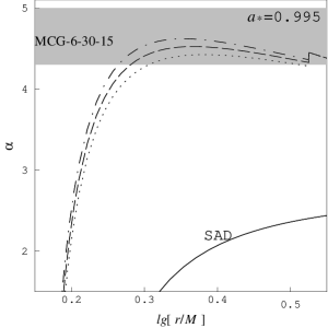
      (a)

      (b)

Figure 8: The emissivity index $\alpha$ versus $\lg(r/M)$ with $\xi_{out}=2.5$ and $n=6,\mbox{ }7$ and $8$ in dotted, dashed and dot-dashed lines, respectively. The emissivity index of the Seyfert 1 galaxy MCG-6-30-15 inferred from the observation of XMM-Newton is shown by the shaded region. The emissivity index of a standard accretion disc (SAD) is plotted in solid line. (upper panel) $a_{*}=0.995$ , (lower panel) $a_{*}=0.998$.

Equation (61) was derived based on the three laws of conservation, and it is proved to be valid for the MC process in Li02a. Combining equations (50) and (61), we can express the contribution to $W_{\varphi}^{r}$ as follows:

$$W_{\varphi}^{r}=\left({W_{\varphi}^{r}}\right)_{DA}+\left({W_{\varphi}^{r}}\right)_{MC},$$ (62)

       (a)                                                   (b)                                                  (c)

Figure 9: The curves of $R_{F}$ versus $\xi$ for $1<\xi<\xi_{out}$ with $n=1.1,1.5$ and $3.0$ in solid, dashed and dotted lines, respectively. (a) $a_{*}=0.1$, (b) $a_{*}=0.328$, (c) $a_{*}=0.998$.

where $\left({W_{\varphi}^{r}}\right)_{DA}$ and $\left({W_{\varphi}^{r}}\right)_{MC}$ are the contribution due to disc accretion and the MC process, and are related to $F_{DA}$ and $F_{MC}$ by equation (61), respectively. Since the flux of angular momentum transferred away from the disc by radiation (henceforth FAMFD) is $F_{MC}L^{+}$, and that transferred from the BH into the disc by the magnetic field (henceforth FAMFH) is $H$, the ratio of the two can be expressed as

$$\begin{array}[]{l}R_{F}\equiv\frac{F_{MC}L^{+}}{H}\\ \\ =-\frac{L^{+}}{Hr}\frac{d\Omega_{D}}{dr}\left({E^{+}-\Omega_{D}L^{+}}\right)^{-2}\int_{r_{ms}}^{r}{\left({E^{+}-\Omega_{D}L^{+}}\right)Hrdr}.\end{array}$$ (63)

From equations (63) we obtain the curves of $R_{F}$ versus $\xi$ for the given values of $n$ and $a_{*}$ as shown in Fig.9.

Combining Figs.6 and 9, we obtain the following relations between FAMFD and FAMFH:

(i)As shown in Fig.9(a), we have $0<R_{F}<1$, which means that the absolute value of FAMFD is less than that of FAMFH, i.e. $H<F_{MC}L^{+}<0$, for a BH with low spin such as $a_{*}=0.1$.

(ii)As shown in Fig.9(b), we have $0<R_{F}<+\infty$ and $-\infty<R_{F}<0$, and $R_{F}$ approaches infinity at the place where $H$ changes its sign. So we infer that $F_{MC}L^{+}<0$ holds in the whole MC region $1<\xi<\xi_{out}$ by considering the sign of $H$ in Fig.6(b).

(iii)As shown in Fig.9(c), we have $0<R_{F}<1$ for $\xi_{in}<\xi<\xi_{eq}$, where FAMFD is dominated by FAMFH. And we have $R_{F}>1$ for $\xi_{eq}<\xi<\xi_{out}$, where FAMFD dominates over FAMFH. It is easy to obtain that the radial coordinate $\xi_{eq}$ indicating $R_{F}=1$ is equal to 1.498, 1.552 and 1.857 for $n=$1.1, 1.5 and 3.0, respectively.

From the above discussion we find that both FAMFD and FAMFH are related intimately not only to the BH spin but also to the disc location.

5 SUMMARY

In this paper the transfer of energy and angular momentum between a rotating BH and its surrounding accretion disc is discussed in detail by considering MC effects. Our discussion is given for two cases: (i)the MC process without disc accretion, (ii)the MC process with disc accretion. In the first case only the two conservation laws of energy and angular momentum are used, while in the second case the conservation of accreted mass is used in addition. Compared with Li02a and Li02b, the mapping relation (19) is used to depict the MC process throughout this paper, and the correlation of some parameters with MC effects is discussed, where the BH spin $a_{*}$, the power-law index $n$ and the radial coordinate $\xi$ are involved.

Compared with the BZ process we find that the MC effects do not increase monotonically as the BH spin. For example, in Figs. 4 and 5 both $\left({rate}\right)_{S}$ and $\eta_{{}_{MC}}$ attain their maxima and then decrease very rapidly as $a_{*}$ approaches unity. These results can be explained by the equations (40) and (49) with the behavior of $\xi_{out}$ as $a_{*}$ approaches unity. From Fig.2 we find that the outer radius of MC region approaches the inner edge of the disc very closely as $a_{*}$ approaches unity, and accordingly the ratio $\beta\equiv{\Omega_{D}}\mathord{\left/{\vphantom{{\Omega_{D}}{\Omega_{H}}}}\right.\kern-1.2pt}{\Omega_{H}}$ approaches unity along as $r_{ms}$ approaches the horizon radius $r_{{}_{H}}$.

Acknowledgments. This work was supported by the National Natural Science Foundation of China under Grant No. 10173004 and No. 10121503. The anonymous referee is thanked for his suggestion on modification of the mapping relation (19).

References

• [1] Blandford R. D., 1976, MNRAS, 176, 465
• [2] Blandford R. D., Znajek R. L., 1977, MNRAS, 179, 433
• [3] Blandford R. D., 1999, in Scllwood J. A., Goodman J., eds, ASP Conf. Ser. Vol. 160, Astrophysical Discs: An EC Summer School, Astron. Soc. Pac., San Francisco, p.265
• [4] Ghosh P., Abramowicz M. A., 1997, MNRAS 292, 887
• [5] Li L. -X. 2000, ApJ, 533, L115
• [6] Li L. -X. 2002, ApJ, 567, 463 (Li02a)
• [7] Li L. -X. 2002, A&A, 392, 469 (Li02b)
• [8] Li L. -X., Paczynski B., 2000, ApJ, 534, L 197
• [9] Macdonald D., Thorne K. S., 1982, MNRAS, 198, 345 (MT)
• [10] Moderski R., Sikora M., Lasota J.P., 1997, in “Relativistic Jets in AGNs” eds.M. Ostrowski, M. Sikora, G. Madejski & M. Belgelman, Krakow, p.110
• [11] Novikov, I. D., & Thorne, K. S., 1973, in Black Holes, ed. Dewitt C (Gordon and Breach, New York) p.345
• [12] Page D. N., Thorne K. S., 1974, ApJ, 191, 499 (PT74)
• [13] Thorne K. S., Price R. H., Macdonald D. A., 1986, Black Holes: The Membrane Paradigm, Yale Univ. Press, New Haven
• [14] Wald R. M., 1984, General Relativity, Chicago Univ. Press, Chicago
• [15] Wang D. X., Xiao K., Lei W. H., 2002, MNRAS, 335, 655 (WXL)