Spiderweb Masks for High-Contrast Imaging

Abstract

Motivated by the desire to image exosolar planets, recent work by us and others has shown that high-contrast imaging can be achieved using specially shaped pupil masks. To date, the masks we have designed have been symmetric with respect to a cartesian coordinate system but were not rotationally invariant, thus requiring that one take multiple images at different angles of rotation about the central point in order to obtain high-contrast in all directions. In this paper, we present a new class of masks that have rotational symmetry and provide high-contrast in all directions with just one image. These masks provide the required $10^{-10}$ level of contrast to within $4\lambda/D$, and in some cases $3\lambda/D$, of the central point, which is deemed necessary for exo-solar planet finding/imaging. They are also well-suited for use on ground-based telescopes, and perhaps NGST too, since they can accommodate central obstructions and associated support spiders.

1 Introduction

With more than 100 extrasolar Jupiter-sized planets discovered in just the last decade, there is now great interest in discovering and characterizing Earthlike planets. To this end, NASA is planning to launch a space-based telescope, called the Terrestrial Planet Finder (TPF), sometime in the middle of the next decade. This telescope, which will ultimately be either an interferometer or a coronagraph, will be specifically designed for high-contrast imaging. Earlier studies (Brown et al. (2002)) indicate that a $4$m class coronagraph ought to be able to discover about 50 extrasolar Earth-like planets if the telescope can provide contrast of $10^{-10}$ at a separation of $3\lambda/D$ and that a $4\times 10$m class telescope ought to be able to discover about 150 such planets if it can provide the same contrast at a separation of $4\lambda/D$.

One of the most promising design concepts for high-contrast imaging is to use pupil masks for diffraction control. So far, work in this direction (see Kasdin et al. (2002a); Brown et al. (2002); Spergel (2000); Kasdin et al. (2002b, 2003)) has focused on optimizing masks that are not rotationally symmetric and thus provide the desired contrast only in a narrow annular sector around a star, but at fairly high throughput. A full investigation of a given star then requires multiple images where the mask is rotated between the images so as to ultimately image all around the star. In this paper, we propose a new class of rotationally symmetric pupil masks, which are attractive because they do not require rotation to image around a star. Such masks consist of concentric rings. As we show, they can provide the desired contrast with a reasonable amount of light throughput. However, it is not clear a priori how to support a concentric-ring mask. While the simplest mechanism would be to lay the rings on a glass plate, even a tiny amount of scatter from the glass could destroy the high contrast. It is better to use an opaque structure for support, maintaining the purely binary nature of the mask. We show here that a certain type of spider support can be used without adversely affecting the contrast in the desired working range.

The paper is organized as follows. In the next section, we show how to design high-contrast concentric-ring masks as a two-step optimization process. The first step is to solve a linear programming problem for an optimal apodization. The second step exploits the “bang–bang” nature of the optimal apodization to create a starting point for a local nonlinear search for an optimal mask. With masks in hand, Section 3 is devoted to considering the impact of support spiders on the point spread function and in particular on finding spiders that preserve the high-contrast region. Finally, we discuss how to design masks with central obstructions. Such masks, with their spiders, could be useful for telescopes with on-axis designs such as NGST and a variety of ground-based telescopes. For these, the mask’s spiders could be used to block the spiders supporting the secondary.

2 Concentric-Ring Masks

The image-plane electric field produced by an on-axis point source and an apodized aperture defined by a circularly-symmetric apodization function $A(\sqrt{x^{2}+y^{2}})$ is given by

$$E(\xi,\zeta)=\iint_{S}e^{-2\pi i(x\xi+y\zeta)}A\left(\sqrt{x^{2}+y^{2}}\right)dxdy,$$ (1)

where

$$S=\displaystyle\left\{(x,y):\;0\leq r(x,y)\leq 1/2,\;\theta(x,y)\in\left[0,2\pi\right]\right\},$$ (2)

and $r(x,y)$ and $\theta(x,y)$ denote the polar coordinates associated with point $(x,y)$. Here, and throughout the paper, $x$ and $y$ denote coordinates in the pupil plane measured in units of the aperature $D$ and $\xi$ and $\zeta$ denote angular (radian) deviation from on-axis measured in units of wavelength over aperture ($\lambda/D$) or, equivalently, physical distance in the image plane measured in units of focal-length times wavelength over aperture ($f\lambda/D$). If the apodization function $A()$ takes only the values $0$ and $1$, then the apodization can be realized as an aperture mask.

For circularly-symmetric apodizations and masks, it is convenient to work in polar coordinates. To this end, let $r$ and $\theta$ denote polar coordinates in the pupil plane and let $\rho$ and $\phi$ denote the image plane coordinates:

$$\begin{array}[]{rclrcl}x&=&r\cos\theta\qquad\qquad\xi&=&\rho\cos\phi\\ y&=&r\sin\theta\qquad\qquad\zeta&=&\rho\sin\phi.\end{array}$$ (3)

Hence,

$$x\xi+y\zeta = r\rho(\cos\theta\cos\phi+\sin\theta\sin\phi)$$ (4)

$$= r\rho\cos(\theta-\phi).$$ (5)

The electric field in polar coordinates depends only on $\rho$ and is given by

$$E(\rho) = \int_{0}^{1/2}\int_{0}^{2\pi}e^{-2\pi ir\rho\cos(\theta-\phi)}A(r)rd\theta dr,$$ (6)

$$= 2\pi\int_{0}^{1/2}J_{0}(2\pi r\rho)A(r)rdr,$$ (7)

where $J_{0}$ denotes the $0$-th order Bessel function of the first kind. Note that the mapping from apodization function $A$ to electric field $E$ is linear. Furthermore, the electric field in the image plane is real-valued (because of symmetry) and its value at $\rho=0$ is the throughput of the apodization:

$$E(0)=2\pi\int_{0}^{1/2}A(r)rdr.$$ (8)

The point spread function (psf) is the square of the electric field. The contrast requirement is that the psf in the dark region be $10^{-10}$ of what it is at its center. Because the electric field is real-valued, it is convenient to express the contrast requirement in terms of it rather than the psf, resulting in a field requirement of $\pm 10^{-5}$.

The apodized pupil that maximizes throughput subject to contrast constraints can be formulated as an infinite dimensional linear programming problem:

$$\begin{array}[]{ll}\mbox{maximize }&E(0)\\ \mbox{subject to }&\begin{array}[t]{rll}\displaystyle-10^{-5}E(0)&\leq E(\rho)\leq 10^{-5}E(0),&\qquad\rho_{\mbox{\scriptsize iwd}}\leq\rho\leq\rho_{\mbox{\scriptsize owd}},\\ 0&\leq A(r)\leq 1,&\qquad 0\leq r\leq 1/2,\end{array}\end{array}$$ (9)

where $\rho_{\mbox{\scriptsize iwd}}$ denotes a fixed inner working distance and $\rho_{\mbox{\scriptsize owd}}$ a fixed outer working distance. Discretizing the sets of $r$’s and $\rho$’s and replacing the integrals with their Riemann sums, the problem is approximated by a finite dimensional linear programming problem that can be solved to a high level of precision (see, e.g., Vanderbei (2001)).

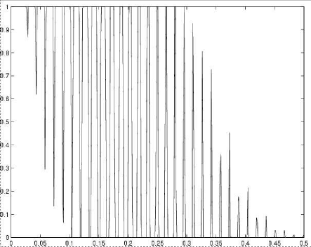
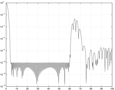
Figure 1: The optimal apodization for $\rho_{\mbox{\scriptsize iwd}}=4$ and $\rho_{\mbox{\scriptsize owd}}=60$ and the associated psf.

The solution obtained for $\rho_{\mbox{\scriptsize iwd}}=4$ and $\rho_{\mbox{\scriptsize owd}}=60$ is shown in Figure 1. Note that the solution is of a bang-bang type. That is, the apodization function is mostly $0$ or $1$ valued. This suggests looking for a mask that is about as good as this apodization. Such a mask can be found by solving the following nonlinear optimization problem. A mask consists of a set of concentric opaque rings, formulated in terms of the inner and outer radii of the openings between the rings:

$$\;[r_{0},r_{1}]$$ first opening (10)

$$\;[r_{2},r_{3}]$$ second opening (11)

$$\;[r_{4},r_{5}]$$ third opening (12)

$$\vdots$$ (13)

$$\;[r_{2m-2},r_{2m-1}] m$$ -th opening (14)

With this notation, the formula for $E(\rho)$ given in (7) can be rewritten as a sum of integrals over these openings:

$$E(\rho) = 2\pi\sum_{k=0}^{m-1}\int_{r_{2k}}^{r_{2k+1}}J_{0}(2\pi r\rho)rdr,$$ (15)

$$= \frac{1}{\rho}\sum_{k=0}^{m-1}\left(r_{2k+1}J_{1}(2\pi r_{2k+1}\rho)-r_{2k}J_{1}(2\pi r_{2k}\rho)\right)$$ (16)

Treating the $r_{k}$’s as variables and using this new expression for the electric field, the mask design problem becomes:

$$\begin{array}[]{ll}\mbox{maximize }&\displaystyle\pi\sum_{k=0}^{m-1}\left(r_{2k+1}^{2}-r_{2k}^{2}\right)\\ \mbox{subject to }&-10^{-5}E(0)\leq E(\rho)\leq 10^{-5}E(0),\qquad\rho_{\mbox{\scriptsize iwd}}\leq\rho\leq\rho_{\mbox{\scriptsize owd}},\\ &0\leq r_{0}\leq r_{1}\leq\cdots\leq r_{2m-1}\leq 1/2.\end{array}$$ (17)

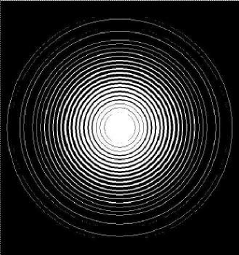
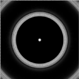
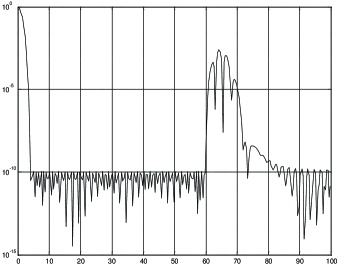
Figure 2: Top. A concentric-ring mask designed to provide high-contrast, $10^{-10}$, from $\lambda/D=4$ to $\lambda/D=60$. Throughput is $0.134=17.00\%$. Bottom. The associated psf.

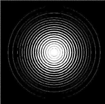
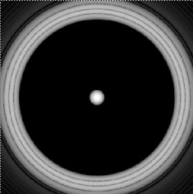
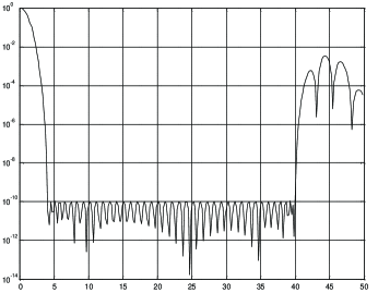
Figure 4: Top. A concentric-ring mask designed to provide high-contrast, $10^{-10}$, from $\lambda/D=4$ to $\lambda/D=40$. Throughput is $0.131=16.62\%$. Bottom. The associated psf.

This problem is a nonconvex nonlinear optimization problem and hence the best hope for solving it in a reasonable amount of cpu time is to use a “local-search” method starting the search from a solution that is close to optimal. The bang-bang solution from the linear programming problem can be used to generate a starting solution. Indeed, the discrete solution to the linear programming problem can be used to find the inflection points of $A$ which can be used as initial guesses for the $r_{k}$’s. The particular local-search method we used is the first-author’s loqo optimizer, which is described in Vanderbei (1999). Figures 2 and 4 show optimal concentric-ring masks computed using an inner working distance of $4$ and two different choices of outer working distances ($40$ and $60$).

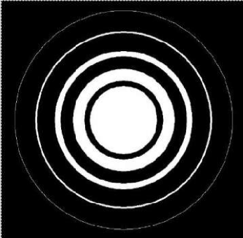
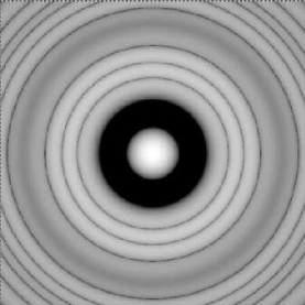
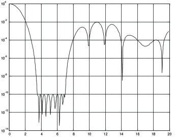
Figure 6: Top. A concentric-ring mask designed to provide high-contrast, $10^{-10}$, from $\lambda/D=3.5$ to $\lambda/D=7$. Throughput is $0.184=23.5\%$. Bottom. The associated psf.

There is great interest in decreasing the inner working distance as this rapidly increases the number of possible planets one could discover via TPF. Or, put another way, it allows one to study the same set of targets but with a smaller aperture instrument. Using $\rho_{\mbox{\scriptsize iwd}}=3.5$, we first tried to solve the linear programming problem with $\rho_{\mbox{\scriptsize owd}}=10$. There is no solution. We next tried $\rho_{\mbox{\scriptsize owd}}=7$ and found a solution to both the linear and nonlinear optimization problems. The resulting mask is shown in Figure 6.

Figure 7 shows a mask with $\rho_{\mbox{\scriptsize iwd}}=3$ and $\rho_{\mbox{\scriptsize owd}}=4.8$. The linear program with $\rho_{\mbox{\scriptsize owd}}=5.0$ is infeasible. We have even created a mask with $\rho_{\mbox{\scriptsize iwd}}=2.5$ and $\rho_{\mbox{\scriptsize owd}}=3.1$. In the interest of space, we don’t show this last mask.

Of course, the obvious issue is ring support. How can the rings be supported without compromising the high-contrast area of the psf, without significantly reducing throughput, and without using glass which would introduce unacceptable scatter? The simplest answer is to use a “spider” similar to those used, for example, to support a secondary mirror. However, spiders create diffraction spikes which can destroy the high-contrast. In the next section, we investigate the effect of spiders and show how to make them in such a way as to preserve high-contrast.

3 Using Spiders for Support

In this section, we study the impact that ring-connecting spiders have on the masks computed in the previous section. Normally, one thinks of a spider as a uniform-width support piece used to hang things. However, there is no specific need that these supports be of uniform width. In fact, since the masks will be made by electroforming technology, such a restriction to uniform width is completely unnecessary. Instead of constant-width spiders, we study constant-angular-width spiders. That is, each spider vane is a narrow sector, starting from a point at the center and flaring out with radius. Incorporating $N$ such spiders uniformly spaced, the electric field, expressed in polar coordinates, is given by

$$E(\rho,\phi)=\displaystyle\iint_{S}e^{-2\pi ir\rho\cos(\theta-\phi)}A(r)rdrd\theta$$ (18)

where

$$A(r)=\sum_{k=0}^{m-1}1_{[r_{2k},r_{2k+1}]}(r),$$ (19)

$$S=\displaystyle\left\{(x,y):\;0\leq r(x,y)\leq 1/2,\;\theta(x,y)\in\Theta\right\},$$ (20)

$$\Theta=\bigcup_{n=0}^{N-1}\left[\frac{2\pi n}{N}+\frac{\alpha}{2},\frac{2\pi(n+1)}{N}-\frac{\alpha}{2}\right],$$ (21)

$\alpha$ denotes the width of a vane in radians, the notation $[a,b]$ denotes the interval on the real line from $a$ to $b$, and the notation $1_{[a,b]}$ denotes the function that is one on the interval $[a,b]$ and zero elsewhere.

The integral in equation (18) can be expressed in terms of Bessel functions using the Jacobi-Anger expansion (see, e.g., Arfken and Weber (2000) p. 681):

$$e^{ix\cos\theta}=\sum_{m=-\infty}^{\infty}i^{m}J_{m}(x)e^{im\theta}.$$ (22)

Substituting into (18), we get:

$$E(\rho,\phi) = \displaystyle\iint_{S}\sum_{m}i^{m}J_{m}(-2\pi r\rho)e^{im(\theta-\phi)}A(r)rdrd\theta$$ (23)

$$= \displaystyle\int_{0}^{1/2}\sum_{m}i^{m}J_{m}(-2\pi r\rho)e^{-im\phi}\left(\int_{\Theta}e^{im\theta}d\theta\right)A(r)rdr$$ (24)

The integral over $\Theta$ is easy to compute:

$$\int_{\Theta}e^{im\theta}d\theta = \sum_{n=0}^{N-1}\int_{\frac{2\pi n}{N}+\frac{\alpha}{2}}^{\frac{2\pi(n+1)}{N}-\frac{\alpha}{2}}e^{im\theta}d\theta$$ (25)

$$= \left\{\begin{array}[]{ll}2\pi-N\alpha&\quad m=0\\ -\frac{2}{j}\sin(jN\frac{\alpha}{2})&\quad m=jN,\;j\neq 0\\ 0&\quad\mbox{otherwise}.\end{array}\right.$$ (29)

Substituting this result into (18), yields

$$E(\rho,\phi) = \int_{0}^{1/2}J_{0}(-2\pi r\rho)(2\pi-N\alpha)A(r)rdr$$ (31)

$$-\sum_{j\neq 0}\int_{0}^{1/2}i^{jN}J_{jN}(-2\pi r\rho)e^{-ijN\phi}\frac{2}{j}\sin(jN\frac{\alpha}{2})A(r)rdr.$$

Lastly, suppose that $N$ is even and use the fact that $J_{-m}(x)=J_{m}(-x)=(-1)^{m}J_{m}(x)$ to get the following expansion for the electric field:

$$E(\rho,\phi) = (2\pi-N\alpha)\int_{0}^{1/2}J_{0}(2\pi r\rho)A(r)rdr$$ (33)

$$-4\sum_{j=1}^{\infty}\int_{0}^{1/2}J_{jN}(2\pi r\rho)\cos(jN(\phi-\pi/2))\frac{1}{j}\sin(jN\frac{\alpha}{2})A(r)rdr.$$

The first term, involving the integral of $J_{0}$, is identical, up to a constant factor, to the formula for the electric field in the absence of spiders. Hence, the impact of the spiders is two-fold: (a) the original electric field is reduced by $1-N\alpha/(2\pi)$ which is just the fraction of the open area that remains uncovered by the spiders, and (b) there are additional terms containing higher order Bessel functions.

For large $N$, the effect of the higher-order Bessel terms becomes negligible for small $\rho$. Indeed, for $x\leq\sqrt{4(m+1)}$,

$$0\leq J_{m}(x)\leq\frac{(x/2)^{m+1}}{(m+1)!},$$ (34)

(which itself follows easily from the alternating Taylor series expansion of the $m$-th Bessel function: $J_{m}(x)=\sum_{l=0}^{\infty}(-1)^{l}(x/2)^{2l+m}/(l!(m+l)!)$). From this we use the Schwarz inequality to estimate the magnitude of the effect of the spiders:

$$\begin{array}[]{rcl}\displaystyle\left|\phantom{\int_{0}^{1/2}}4\sum_{j=1}^{\infty}\int_{0}^{1/2}J_{jN}(2\pi r\rho)\cos(jN(\phi\right.&-&\left.\pi/2))\displaystyle\frac{1}{j}\sin(jN\frac{\alpha}{2})A(r)rdr\phantom{\int_{0}^{1/2}}\right|\\ &\leq&\;\displaystyle\frac{1}{2}\sum_{j=1}^{\infty}J_{jN}(\pi\rho_{\mbox{\scriptsize owd}})\\ &\leq&\;\displaystyle\frac{1}{2}\sum_{j=1}^{\infty}\frac{1}{(jN+1)!}\left(\frac{\pi\rho_{\mbox{\scriptsize owd}}}{2}\right)^{jN+1},\end{array}$$ (35)

for $\rho_{\mbox{\scriptsize owd}}\leq\sqrt{4(N+1)}/\pi$. Since the last bound is dominated by $e^{\pi\rho_{\mbox{\scriptsize owd}}/2}/2$, it follows from the dominated convergence theorem that this last bound tends to zero as $N$ tends to infinity.

The convergence to zero of the terms in the sum on $j$ is very fast. In fact, if $N$ is set large enough that $\max_{0\leq x\leq\pi\rho_{\mbox{\scriptsize owd}}}J_{N}(x)\leq 10^{-5}$, then the $j=1$ term dominates the sum of all the higher-order terms and is itself dominated by the $J_{0}$ term. Figure 9 shows a plot of $J_{50}$, $J_{100}$, and $J_{150}$. These three Bessel functions first reach $10^{-5}$ at $35.2$, $81.0$, and $128.1$, respectively.

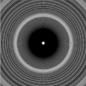
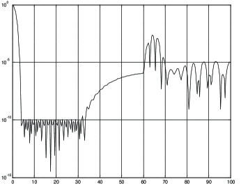
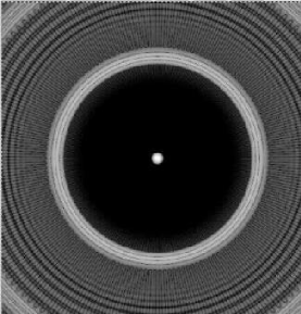
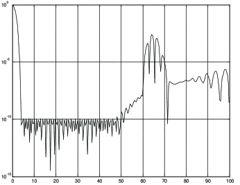
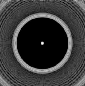
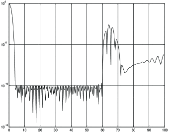
Figure 3: Psf for mask in Figure 2 with spiders. Top Row. $100$ spiders each spanning $0.005$ radians. Second Row. $150$ spiders each spanning $0.003$ radians. Third Row. $180$ spiders each spanning $0.0025$ radians.

Figure 3 shows the psf for the mask designed with $\rho_{\mbox{\scriptsize iwd}}=4$ and $\rho_{\mbox{\scriptsize owd}}=60$ and three different spider configurations. The configuration consisting of 180 spiders each spanning 0.0025 radians completely preserves the full high-contrast region. Note that this spider fills, in total, $180\times 0.0025=0.45$ radians, which is $7.2\%$ of the open area.

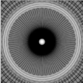
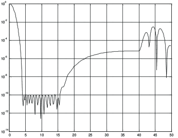
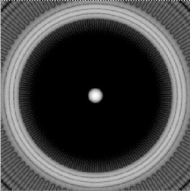
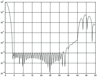
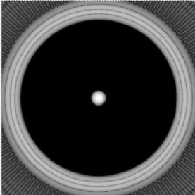
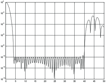
Figure 5: Psf for mask in Figure 4 with spiders. Top Row. $50$ spiders each spanning $0.01$ radians. Second Row. $100$ spiders each spanning $0.005$ radians. Third Row. $120$ spiders each spanning $0.003$ radians.

Figure 5 shows the psf for the mask designed with $\rho_{\mbox{\scriptsize iwd}}=4$ and $\rho_{\mbox{\scriptsize owd}}=40$ and three different spider configurations. The configuration consisting of 120 spiders each spanning 0.003 radians completely preserves the full high-contrast region. Note that this spider fills, in total, $120\times 0.003=0.36$ radians, which is $5.7\%$ of the open area.

For the mask designed with $\rho_{\mbox{\scriptsize iwd}}=3.5$ and $\rho_{\mbox{\scriptsize owd}}=7$ (shown in Figure 6), $50$ spider vanes suffice to preserve the high-contrast of the dark zone. The resulting psf is indistinguishable from the one shown in Figure 6. If each spider spans $0.01$ radians then they fill, in total, $50\times 0.01=0.5$ radians, which is $8.0\%$ of the open area.

For the mask designed with $\rho_{\mbox{\scriptsize iwd}}=3.0$ and $\rho_{\mbox{\scriptsize owd}}=4.8$ (shown in Figure 7), again $50$ spider vanes suffice to preserve the high-contrast of the dark zone and the resulting psf is indistinguishable from the one shown in the earlier figure.

None of the masks presented have a central obstruction. Hence, there are many spiders all coming to a point at the center. This central area is probably the hardest part of the mask to manufacture. One probably needs to add a small bead at the center as an attachment point for the spiders. Using the same inner and outer working distances ($3.0$ and $4.8$) as for the mask in Figure 7, we experimented with adding a constraint to the optimization problem that forces there to be a small central obstruction. In the nonlinear optimization model, the constraint simply amounts to fixing $r_{0}$ to a specified small value. We tried several values and found that we could fix $r_{0}$ to $0.01$ (i.e., a $2\%$ obstruction) and still find an optimal solution with essentially an unchanged throughput.

It is a trivial matter to make designs with larger central obstructions to accomodate, say, a secondary mirror in an on-axis design. However, once the central obstruction becomes large, one loses the ability to get tight inner working distances. Figure 8 shows a design for a $31\%$ central obstruction, an inner working distance of $\rho_{\mbox{\scriptsize iwd}}=10$ and an outer working distance of $\rho_{\mbox{\scriptsize owd}}=40$. With $\rho_{\mbox{\scriptsize iwd}}=9$, the linear optimization problem has a solution but not the nonlinear one. With $\rho_{\mbox{\scriptsize iwd}}=8$, not even the linear optimization problem has a solution.

Some TPF concepts involve an elliptical pupil geometry since this might provide a means to achieve improved angular resolution in realizable rocket fairings. The designs presented in this paper are given in unitless variables. When re-unitizing, a different scale can be used for the $x$ and $y$ directions. In this way, these designs can be applied directly to elliptical pupils. Of course, the high-contrast region of the psf will also be elliptical with the short axis of the psf corresponding to the long axis of the pupil.

4 Final Remarks

There are two parts to TPF: discovery and characterization. Discovery refers to the simple act of looking for exosolar planets. Characterization refers to the process of learning as much as possible about specific planets after they have been discovered. The masks presented here are intended primarily for discovery since a single exposure with these masks can discover a planet in any orientation relative to its star. However, once a planet is found and its orientation is known, some of the asymmetric masks presented in previous papers will be used for photometry and spectroscopy as they have higher single-exposure throughput.

An alternative to pupil masks is to use a traditional coronagraph, which consists of an image plane mask followed by a Lyot stop in a reimaged pupil plane. Recently, Kuchner and Traub (2002) have developed band-limited image-plane masks that achieve the desired contrast to within $3\lambda/D$. However, this approach suffers from sensitivity to pointing accuracy. Nonetheless, the approach is promising. In the future, we plan to consider combining pupil masks with image masks and Lyot stops to make a hybrid design that hopefully will provide a design achieving the desired contrast with an even smaller inner working distance.

In this paper we have only considered scalar electric fields. We leave the important and more complex issue of how to treat vector electric fields, i.e. polarized light, to future work.

Acknowledgements. We would like to express our gratitude to our colleagues on the Ball Aerospace and Technology TPF team. We benefited greatly from the many enjoyable and stimulating discussions. This work was partially performed for the Jet Propulsion Laboratory, California Institute of Technology, sponsored by the National Aeronautics and Space Administration as part of the TPF architecture studies and also under contract number 1240729. The first author received support from the NSF (CCR-0098040) and the ONR (N00014-98-1-0036).

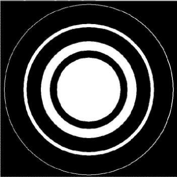
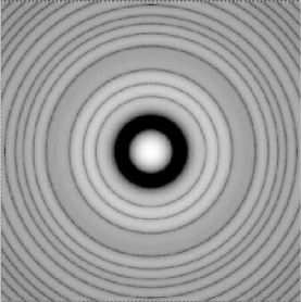
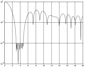
Figure 7: Top. A concentric-ring mask designed to provide high-contrast, $10^{-10}$, from $\lambda/D=3.0$ to $\lambda/D=4.8$. Throughput is $0.251=31.9\%$. Bottom. The associated psf.

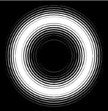
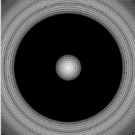
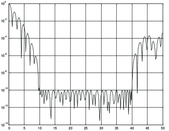
Figure 8: Top. A concentric-ring mask accomodating a large central obstruction. High contrast of $10^{-10}$, from $\lambda/D=10.0$ to $\lambda/D=40$. Bottom. The associated psf.

Figure 9: The Bessel functions $J_{50}$, $J_{100}$, and $J_{150}$. They first reach $10^{-5}$ at $35.2$, $81.0$, and $128.1$, respectively.

References

- Arfken and Weber (2000) G.B. Arfken and H.J. Weber. Mathematical Methods for Physicists. Harcourt/Academic Press, 5th edition, 2000.
- Brown et al. (2002) R. A. Brown, C. J. Burrows, S. Casertano, M. Clampin, D. Eggets, E.B. Ford, K.W. Jucks, N. J. Kasdin, S. Kilston, M. J. Kuchner, S. Seager, A. Sozzetti, D. N. Spergel, W. A. Traub, J. T. Trauger, and E. L. Turner. The 4-meter space telescope for investigating extrasolar earth-like planets in starlight: TPF is HST2. In Proceedings of SPIE: Astronomical Telescopes and Instrumentation, number 14 in 4860, 2002.
- Kasdin et al. (2002a) N. J. Kasdin, D. N. Spergel, and M. G. Littman. An optimal shaped pupil coronagraph for high contrast imaging, planet finding, and spectroscopy. submitted to Applied Optics, 2002a.
- Kasdin et al. (2002b) N.J. Kasdin, R.J. Vanderbei, D.N. Spergel, and M.G. Littman. Optimal Shaped Pupil Coronagraphs for Extrasolar Planet Finding. In Proceedings of SPIE Conference on Astronomical Telescopes and Instrumentation, number 44 in 4860, 2002b.
- Kasdin et al. (2003) N.J. Kasdin, R.J. Vanderbei, D.N. Spergel, and M.G. Littman. Extrasolar Planet Finding via Optimal Apodized and Shaped Pupil Coronagraphs. Astrophysical Journal, 2003. To appear.
- Kuchner and Traub (2002) M. J. Kuchner and W. A. Traub. A coronagraph with a band-limited mask for finding terrestrial planets. The Astrophysical Journal, (570):900+, 2002.
- Spergel (2000) D. N. Spergel. A new pupil for detecting extrasolar planets. astro-ph/0101142, 2000.
- Vanderbei (1999) R.J. Vanderbei. LOQO user’s manual—version 3.10. Optimization Methods and Software, 12:485–514, 1999.
- Vanderbei (2001) R.J. Vanderbei. Linear Programming: Foundations and Extensions. Kluwer Academic Publishers, 2nd edition, 2001.