On the Angular Correlation Function of SZ Clusters :
Extracting cosmological information from a 2D catalog

We discuss the angular correlation function of Sunyaev–Zel’dovich (SZ)–detected galaxy clusters as a cosmological probe. As a projection of the real–space cluster correlation function, the angular function samples the underlying SZ catalog redshift distribution. It offers a way to study cosmology and cluster evolution directly with the two–dimensional catalog, even before extensive follow–up observations, thereby facilitating the immediate scientific return from SZ surveys. As a simple illustration of the information content of the angular function, we examine its dependence on the parameter pair $(\Omega_{\rm M},\sigma_{8})$ in flat cosmologies. We discuss sources of modeling uncertainty and consider application to the future Planck SZ catalog, showing how these two parameters and the normalization of the SZ flux–mass relation can be simultaneously found when the local X–ray cluster abundance constraint is included.

1 Introduction

The Sunyaev–Zel’dovich (SZ) effect (Sunyaev & Zel’dovich 1970, 1972) has become a practical observational tool for studying galaxy clusters and cosmology (for recent reviews see Birkinshaw 1999; Carlstrom et al. 2002). Current observations of individual clusters, when combined with X–ray observations, constrain cosmological parameters via gas mass fractions (Grego et al. 2002) and angular–diameter distance determinations (Mason et al. 2001; Jones et al. 2001; Reese et al. 2002). Multi–band millimeter observations of a handful of clusters have already been used to set limits on peculiar velocities (Holzapfel et al. 1997; Benson et al. 2003), and theoretical studies of this technique show its promise for the future (Aghanim et al. 2002a, 2002b; Holder 2002). A new generation of optimized, dedicated instruments, both large–format bolometer arrays and interferometers with high sensitivity receivers, will qualitatively improve these studies. And the arrival of these instruments within the next few years, in addition to the Planck mission, will move the field forward to its next important step: surveying. This will open a new observational window onto large–scale structure and its evolution out to large redshifts.

The ultimate goal of these SZ surveys is the construction of large cluster catalogs with multi–wavelength follow–up observations in order to perform cosmological studies; for example, constraining cosmological parameters with the counts and redshift distribution (e.g., Barbosa et al. 1996; Eke et al. 1996; Colafrancesco et al. 1997; Haiman et al. 2001; Holder et al. 2001; Kneissl et al. 2001; Weller et al. 2002; Benson et al. 2002). Driving this effort are the particular advantages of SZ–based cluster catalogs (Bartlett 2000; Bartlett 2001): Firstly, SZ surveys are intrinsically efficient at finding clusters at large redshift, due to the surface brightness constancy of the SZ effect. The thermal SZ spectrum is furthermore universal, the same for all clusters at any redshift. Other emission mechanisms, in contrast, suffer from cosmological dimming and the need for accurate $k$–corrections. Secondly, SZ surveys select clusters based on their thermal energy. Since the spectrum is the same for all clusters, the total observable SZ flux from a cluster can be expressed in a frequency independent manner as the integrated Compton $y$–parameter, $Y=\int d\Omega\;y(\hat{n})$, where the integral is over the cluster profile (see Equation 4 below). The $y$ parameter being the pressure integrated along the line–of–sight ($y\propto\int dl\;nT)$, this then implies $Y\propto MT$, i.e., the thermal energy of the intracluster medium (ICM). This is important, because the total thermal energy of the ICM is given by energy re-partition during cluster collapse and is independent of any thermal or spatial structure in the gas. It is hence a more robust quantity than, for example, the X–ray emission measure that depends in a more complicated fashion on both the ICM density and temperature. Hydrodynamical simulations confirm this expectation by showing a tight SZ flux–mass relationship with little scatter (da Silva et al. 2003). Object selection in a flux–limited SZ catalog is therefore relatively easy to interpret in terms of cluster mass and redshift. For instance, it is easy to show that the minimum detectable cluster mass is almost independent of redshift. This is particularly advantageous for evolutionary studies, because one is able to follow the evolution of the same kind of object over redshift, instead of comparing massive objects at high redshift to less massive ones at low redshift, as is the case with X–ray samples.

Detailed follow–up of SZ surveys will, however, be time–consuming, and an enormous effort for the more than $10^{4}$ clusters expected from Planck. Large–area photometric surveys in the optical and infrared (e.g., SDSS) will help (Bartelmann & White 2002), but it is important to identify the kind of science that may be done directly with the two dimensional catalog of cluster positions and SZ fluxes, what we will refer to in the following as the SZ photometric catalog. This will certainly be the first science to be performed. Source counts represent the primary avenue of 2D study that has been discussed extensively in the literature. In this paper, we examine the next higher order catalog statistic, namely, the angular correlation function $w(\theta)$ of SZ–detected clusters (Diaferio et al. 2003). We quantify its information content and study its potential use as a cosmological probe. The angular function samples the catalog redshift distribution, because it is a projection of the real–space correlation function along the line–of–sight. With an appropriate model for the real–space correlation function of the catalog, we may gain some insight on this distribution, and hence on the underlying cosmological model.

Moscardini et al. (2002) studied the 3D clustering properties of SZ detected clusters, taking the Planck survey as an example and accounting for evolutionary effects along the past light–cone. Diaferio et al. (2003) examined the angular function of SZ clusters as a means of identifying probable physical cluster pairs (in 3D) and superclusters. Our modeling is similar to theirs, although we focus instead on the angular function as a cosmological probe permitting the extraction of cosmological information from a photometric SZ catalog. The idea is of course not new, and has been applied in the past to, for example, optical and X–ray cluster catalogs; but we reiterate the advantages of an SZ catalog in this context: the cluster selection function is relatively easy to model (compared to other observing bands), and it extends out to large redshift, giving a longer base–line for viewing evolutionary effects.

We should distinguish at the outset the difference between the angular power spectrum, $C^{\rm sz}_{l}$, of SZ–induced temperature fluctuations (secondary anisotropies in the cosmic microwave background [CMB]) and the angular correlation function of detected clusters in a SZ survey, $w(\theta)$. The angular power spectrum $C^{\rm sz}_{l}$ is a two–point statistic quantifying the integrated contribution of the entire cluster population to the CMB sky brightness fluctuations. It is dominated by the Poisson term and its overall shape is determined by the mean SZ profile of clusters. Cluster–cluster correlations add additional power on the order of $20-30$% of the pure Poisson term (Komatsu & Kitayama 1999). Since it is defined relative to the mean cosmic microwave background temperature, we expect the SZ fluctuation power to increase with the surface density of clusters on the sky. This is quantitatively confirmed by both numerical simulations and analytical calculations that indicate $C^{\rm sz}_{l}\propto\sigma_{8}^{7}$ (all other factors held constant), where $\sigma_{8}$ is the amplitude the density perturbations, the quantity most directly influencing cluster abundance. The fluctuation power spectrum is an analysis method appropriate in a low signal–to–noise context (the current situation) where individual source identification is not possible. Fluctuations induced by the SZ effect have been invoked as a possible explanation for the excess power at high multipole $l$ reported by the CBI collaboration (Bond et al. 2002) and consistent with new VSA data (Grainge et al. 2002). If this were entirely due to the cluster population, it would imply a surprisingly large value for $\sigma_{8}$ ($>1$; Bond et al. 2002; Komatsu & Seljak 2002; Holder 2002), although an important contribution from heated gas at reionization may also be expected (Oh et al. 2003).

The angular function $w(\theta)$ quantifies the projected clustering of a 2D catalog of individually detected clusters. It refers to the object positions and makes no reference to the mean background sky brightness. There are several ways to imagine using the information contained in the SZ cluster angular function (e.g., Diaferio et al. 2003). In the following we choose to illustrate its use by examining constraints on the matter density $\Omega_{\rm M}$ and $\sigma_{8}$ in the context of flat CDM–like models. The SZ counts provide one constraint on a combination of these parameters. To extract additional information from the 2D catalog using the angular function, we are forced to model the real–space cluster correlation function. In CDM scenarios, clusters form from peaks in the density field whose clustering may be analytically calculated. We adopt the approach proposed by Mo & White (1996; 2002). Any conclusions that we draw are, therefore, unavoidably dependent on this clustering model (Moscardini et al. 2002; Diaferio et al. 2003); however, it is well founded in the context of CDM cosmogonies and compares well with the results of numerical simulations, at least at redshifts lower than $\sim 10$ (Reed et al. 2003; Jenkins et al. 2001). Another important issue concerns the modeling of the intracluster medium. Moscardini et al. (2002), for example, find non–negligible dependence of the 3D correlation function on ICM properties. We discuss the issue below for the angular function, but we note here that it tends to be dominated by massive clusters (depending of course on the exact flux limit; see below) that follow relatively well observed scaling laws. As we show, adding constraints from the local X–ray cluster abundance permits us to simultaneously constrain the cosmological parameters and the cluster baryon content.

In the following section, we give our master equation for calculating $w(\theta)$ and identify the necessary modeling ingredients. We outline our cluster model in Section 3. Results for the angular function are presented in Section 4, where we apply the results to constraining the cosmological parameters $\sigma_{8}$ and $\Omega_{\rm M}$. We discuss the influence of ICM physics on the results and how to use additional information from the local cluster abundance to simultaneously constrain this physics and the cosmology. Our fiducial example is the Planck mission. Section 5 closes with a final discussion and summary.

2 The Angular Correlation Function

In this section we relate the angular correlation function to the real–space correlation function in the context of SZ observations. The 3–dimensional (auto)correlation function $\xi$ quantifies the 2–point clustering of a population in terms of the probability in excess of Poisson of finding two objects at a separation $r$. The angular correlation $w(\theta)$ of the same population is the projection of $\xi$ onto the sky:

$$d\Omega_{1}d\Omega_{2}\Sigma^{2}[1+w(\theta)]=$$ (1)

$$d\Omega_{1}d\Omega_{2}\int dz_{1}dz_{2}\frac{dV_{1}}{d\Omega_{1}dz_{1}}\frac{dV_{2}}{d\Omega_{2}dz_{2}}\times$$

$$\int dM_{1}dM_{2}\frac{dn_{1}}{dM_{1}}\frac{dn_{2}}{dM_{2}}(1+\xi)$$

where the integrals concern two lines–of–sight (los) of solid angles $d\Omega_{1}$ and $d\Omega_{2}$ separated on the sky by angle $\theta$. In this expression, $dn/dM$ represents the cluster mass function, and we assume the small angle approximation here and throughout. The surface density of sources (the counts) with integrated Compton parameter larger than $Y_{\rm lim}$ (the SZ ‘flux’ limit; see the following section, Equation 4) is given by

$$\Sigma(Y_{\rm lim})=\int_{0}^{\infty}dz\frac{dV}{d\Omega dz}\int_{M_{\rm lim}(Y_{\rm lim},z)}^{\infty}dM\frac{dn}{dM}(M,z)$$ (2)

The correlation function $\xi$ depends on cluster mass, redshift and, according to statistical isotropy, on physical separation $r(\theta)=r_{1}^{2}(z_{1})+r_{2}^{2}(z_{2})-2r_{1}r_{2}\cos(\theta)$, where $r_{1}$ and $r_{2}$ are angular–diameter distances. Assuming that correlations fall off sufficiently rapidly with distance, as is observed, we may take the two clusters to be at approximately the same redshift and write $\xi[M_{1},M_{2},z,r(\theta)]$. We furthermore adopt a linear biasing scheme in which $\xi(M_{1},M_{2},z,r)=b(M_{1},z)b(M_{2},z)\xi_{\rm dm}(z,r)$, where $\xi_{\rm dm}(z,r)$ is the correlation function of the underlying cold dark matter and $b(M,z)$ is the bias factor for clusters (see below). Then, using the short–hand notation $\phi(M,z,Y_{\rm lim})=(1/\Sigma)b(M,z)(dV/dzd\Omega)dn/dM$ for the joint distribution of clusters in mass and redshift, weighted by the bias factor, we arrive at the expression

$$w(\theta,Y_{\rm lim})=$$

$$\int_{0}^{\infty}dz\int\int_{M_{\rm lim}(Y_{\rm lim},z)}^{\infty}dM_{1}dM_{2}\;\phi(M_{1},z)\phi(M_{2},z)\times$$

$$\int dr\frac{dz}{dr}(z)\xi_{\rm dm}[z,r(\theta)]$$

$$\equiv\int_{0}^{\infty}dz\Phi^{2}(z,Y_{\rm lim})\int dr\frac{dz}{dr}(z)\xi_{\rm dm}[z,r(\theta)]$$

a sort of Limber’s equation appropriate for SZ sources (Limber 1953; Peebles 1993; Diaferio et al. 2003) in which we explicitly show the dependence on limiting flux $Y_{\rm lim}$. From this equation we clearly see that the three key ingredients are the the mass–limit function $M_{\rm lim}(z,Y_{\rm lim})$, the distribution function $\phi$ and the correlation function $\xi_{\rm dm}$. We now discuss our modeling of each.

3 The SZ Population

The SZ cluster population inherits its properties from two sources: its constituent dark matter halos, whose properties are the sole result of gravitational evolution, and the relationship between observable SZ flux and these halos, governed by more difficult to model baryonic physics. It is reasonable to characterize dark halos by their mass and redshift, and we will apply the results of N–body simulations that give both their abundance (i.e., the mass function) and spatial correlations (i.e., clustering bias $b(M,z)$ and the correlation function $\xi_{\rm dm}$) as a function of these two fundamental descriptors. More difficult to model, the baryonic physics of the cluster gas requires particular attention to various (and at times contradictory) observational constraints and theoretical scaling laws.

3.1 Halo properties

The abundance of galaxy clusters is given by the mass function of collapsed objects, which is completely specified once the linear power spectrum of dark matter perturbations is specified. For the latter we adopt the BBKS (Bardeen et al. 1986) transfer function (see also below), while for the mass function we employ the fitting formula (improved Press–Schechter) given by Sheth & Tormen (1999):

$$\frac{dn}{dM}(M,z)dM=A\left(1+\frac{1}{\nu^{\prime 2q}}\right)\sqrt{\frac{2}{\pi}}\frac{\overline{\rho}}{M}\frac{d\nu^{\prime}}{dM}\exp\left(\frac{-\nu^{\prime 2}}{2}\right)dM$$ (3)

where $\overline{\rho}$ is the universal mean mass density and the constants $A\approx 0.322$ and $q=0.3$; the parameter $\nu^{\prime}=\sqrt{a}\nu$, where $\nu\equiv\frac{\delta_{c}}{D(z)\sigma(M)}$ is the usual critical peak height ($\delta_{c}\approx 1.69$) normalized to the mass–density perturbation variance $\sigma(M)$ in spheres containing mass $M$, and the constant $a=0.707$. The expression for the growth factor for flat models with $\Lambda>0$ is taken from Carroll et al. (1992):

$$D(z,\Omega_{\rm M},\Omega_{\Lambda})= \frac{g(z)}{g(0)(1+z)}$$

$$g(z,\Omega_{\rm M},\Omega_{\Lambda})\approx \frac{5}{2}\Omega_{\rm M}(z)[\Omega_{\rm M}(z)^{4/7}-$$

$$-\Omega_{\Lambda}(z) +(1+\Omega_{\rm M}(z)/2)(1+\Omega_{\Lambda}(z)/70)]^{-1}$$

with the definitions $\Omega_{\rm M}(z)\equiv\Omega_{\rm M}(1+z)^{3}/E^{2}(z)$, $\Omega_{\Lambda}(z)\equiv\Omega_{\Lambda}/E^{2}(z)$, and $E^{2}(z)=[\Omega_{\Lambda}+(1-\Omega_{\rm M}-\Omega_{\Lambda})(1+z)^{2}+\Omega_{\rm M}(1+z)^{3}]$; $\Omega_{M}$ and $\Omega_{\Lambda}$ written without an explicit redshift dependence will indicate present–day values ($z=0$).

As mentioned above, we use a linear bias scheme to relate the cluster–cluster correlation function to that of the dark matter and employ the analytic fitting formula for $b(M,z)$ given by Sheth et al. (2001); the formula includes corrections for ellipsoidal perturbation collapse:

$$b(M,z)=1+\frac{1}{\sqrt{a}\delta_{c}(z)}\left[\sqrt{a}(a\nu^{2})+\sqrt{a}b(a\nu^{2})^{1-c}\right]-$$

$$-\frac{(a\nu^{2})^{c}}{(a\nu^{2})^{c}+b(1-c)(1-c/2)}$$

where $\delta_{c}$, $\nu$ and $a$ are given above, and $b=0.5$ and $c=0.6$. We model the linear dark matter perturbation spectrum with the BBKS transfer function with shape parameter fixed at $\Gamma=0.25$ and scale–invariant primordial density fluctuations ($n=1$). This seems to provide a good fit to galaxy clustering data (Percival et al. 2001) and is consistent with constraints on $n$ from CMB anisotropies (Spergel et al. 2003, and references therein). The resulting linear theory $\xi_{\rm dm}$ is adequate on most scales ($\theta>10\arcmin$), although we also include non–linear corrections according to the fitting formula developed by Peacock & Dodds (1996).

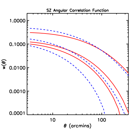
Figure 1: Angular correlation function of SZ detected clusters calculated in two different flat models ($\Omega_{\rm M}=0.3$ and $\sigma_{8}=0.9$ as the dashed lines, and $\Omega_{\rm M}=1$ and $\sigma_{8}=0.7$ as the solid lines) for three flux limits ($Y_{\rm lim}=10^{-3}$, $10^{-4}$, $10^{-6}$ arcmin², decreasing from top to bottom). The models adopt the same linear matter power spectrum (shape parameter $\Gamma=0.25$) and $Y_{*}=7.6\times 10^{-5}h^{7/6}$ arcmin² (see text).

3.2 Intracluster Medium

With the abundance and clustering of halos now specified, we next relate the observable SZ flux to cluster mass and redshift. This relation is particularly robust from a theoretical viewpoint, contrary to, for example, the situation for X–ray luminosity. In the non–relativistic regime, the surface brightness of the thermal SZ effect – measured relative to the mean sky intensity – at position $\hat{\Omega}$ on a cluster image is

$$\Delta i_{\nu}(\hat{\Omega})=y(\hat{\Omega})j_{\nu}$$

where the Compton $y$ parameter is an integral of the pressure along the line–of–sight

$$y(\hat{\Omega})=\int_{los\;\hat{\Omega}}dl\frac{kT}{mc^{2}}n\sigma_{T}$$

with $T$ the gas temperature (strictly speaking, that of the electrons), $\sigma_{T}$ the Thompson cross section, $k$ and $m$ the Boltzmann constant and the electron mass, respectively, and where $j_{\nu}$ is a universal spectral function that is the same for all clusters, independent of their properties (Birkinshaw 1999). Since the thermal SZ spectrum is the same for all clusters, we may express the total flux in a frequency independent manner using the integrated Compton parameter $Y=\int d\Omega\;y(\hat{\Omega})$, where the integral is over the cluster profile. The total flux density (e.g., in Jy) is then $S_{\nu}=Yj_{\nu}$. This is the total flux (density) measured by an experiment with low angular resolution in which clusters are simply point sources. From these definitions, we find that the observable flux is directly proportional to the total thermal energy of the ICM (e.g., Barbosa et al. 1996):

$$Y(M,z)=\frac{k\sigma_{T}}{mc^{2}}\frac{N_{\rm e}T}{D_{\rm ang}^{2}(z)}\propto\frac{f_{\rm gas}(M,z)T(M,z)M}{D_{\rm ang}^{2}(z)}$$ (4)

where $N_{\rm e}$ is the total number of electrons, $f_{\rm gas}$ is the ICM mass fraction, $D_{\rm ang}(z)=H_{\rm o}^{-1}d_{\rm ang}(z)$ is the angular diameter distance, and $T$ is to be understood as the mean (particle, and not emission–weighted) electron temperature; note that with this understanding, the relation does not depend on any assumption of isothermality. It is this direct relation between observable SZ flux and thermal gas energy that lies at the heart of some of the advantages of SZ over X–ray surveys (Bartlett 2001).
We have taken care to write the quantities $f_{\rm gas}$ and $T$ as general functions of mass and redshift. In the absence of efficient heating/cooling and gas reprocessing, the cluster population will be fully self–similar. Simple theoretical arguments based on energetics during collapse suggest in this case the existence of a scaling law between cluster temperature and mass:

$$T(M,z)=T_{*}\left(M_{15}h\right)^{2/3}\left(\Delta(z)E(z)^{2}\right)^{1/3}\left[1-2\frac{\Omega_{\Lambda}(z)}{\Delta(z)}\right]$$ (5)

adopting the notation of Pierpaoli et al. (2002). In this expression, the mass $M_{15}$ is measured in units of $10^{15}\leavevmode\nobreak\$M_⊙, $\Delta(z)$ is the full non–linear overdensity inside the virial radius relative to the critical density ($\sim 178$). In the self–similar model, the gas mass fraction $f_{\rm gas}$ is constant, essentially proportional to the universal ratio $\Omega_{\rm B}/\Omega_{\rm M}$.
These scaling expectations are indeed manifest in hydrodynamical simulations that neglect cooling, and supported by observations of the more massive clusters with cooling timescales longer than the Hubble time (Mohr et al. 1999; Allen et al. 2001; Finoguenov et al. 2001; Xu et al. 2001; Arnaud et al. 2002). Although there is good indication that clusters are a population with rather regular properties, as suggested by these scaling laws, there is also direct evidence that it is not exactly self–similar. Deviations are most pronounced for the lower mass objects ($T<2$ keV), as perhaps expected since they have shorter cooling times and plausible energy injection mechanisms more readily compete with their gravitational energy (Ponman et al. 1999; Lloyd–Davies et al. 2000). More generally, one may write

$$Y(M,z)=Y_{15}(z)M_{15}^{5/3+\alpha}(1+z)^{\gamma}$$ (6)

The factor $Y_{15}(z)$ incorporates all the $z$ dependence of Eqs. (4,5) and is defined such that the self–similar model corresponds to $\alpha=\gamma=0$.

Although we have discussed Eq. (6) via scaling relations for $T$ and $f_{\rm gas}$, it is more pertinent to consider it as a single relation between observable SZ flux and cluster mass and redshift, one that expresses the proportionality between the observable flux and the gas thermal energy. Hydrodynamical simulations incorporating cooling and pre–heating (da Silva et al. 2003) indicate $\alpha$ between 0.1 and 0.2 and $\gamma\approx 0$, with a very tight scatter about the relation, much tighter than corresponding relations for X–ray quantities. This confirms our expectations that the SZ flux is a more robust quantity than its X–ray counterparts. Even though very low mass clusters are included in the fit, only mild deviations from self–similarity in this relation are seen in the simulations. These deviations are most pronounced in the low mass systems, while the higher mass systems appear compatible with the self–similar scaling laws for $T$–$M$ and $f_{\rm gas}$. Caution is still warranted, however, due to the unstable nature of cooling, issues of numerical resolution, and the fact that these codes model the gas as a single phase medium; the simulation volume also contains mostly low mass systems, with only a few clusters with $M_{15}>0.2$. Simulation results are nonetheless roughly consistent with X–ray observations (Borgani et al. 2002; Muanwong et al. 2002).

At our fiducial Planck flux limit of $Y=10^{-4}$ arcmin², we have checked that the counts and value of the angular function at 30 arcmins are little affected by clusters below $T=2$ keV, at least at $\Omega_{M}<0.6$. We therefore concentrate on the self–similar case with $\alpha=\gamma=0$. On the other hand, we consider the normalization of Eq. (6) as a parameter free to vary within certain limits suggested by X–ray observations of $f_{\rm gas}$ and $T$. Moscardini et al. (2002) have argued that this freedom makes it difficult to use only SZ observations to constrain $\sigma_{8}$ and $\Omega_{\rm M}$. To overcome this modeling uncertainty, we combine SZ observations of both the number counts and the angular correlation function with constraints arising from the local abundance of X–ray clusters. We shall find that the three kinds of observations are complementary and lead to constraints on the cosmological parameters.
To give a feel for the order of magnitude, we note that

$$Y_{15}(z) =\left(7.4\times 10^{-5}h^{7/6}\;{\rm arcmin}^{2}\right)\left(\frac{T_{*}}{{\rm keV}}\right)\left(\frac{f_{\rm gas}}{0.07h^{-3/2}}\right)\times$$ (7)

$$\left(\frac{\Delta(z)E(z)^{2}}{178}\right)^{1/3}\left[1-2\frac{\Omega_{\Lambda}(z)}{\Delta(z)}\right]\frac{1}{d_{\rm ang}^{2}(z)}$$

$$\equiv Y_{*}\left(\frac{\Delta(z)E(z)^{2}}{178}\right)^{1/3}\left[1-2\frac{\Omega_{\Lambda}(z)}{\Delta(z)}\right]\frac{1}{d_{\rm ang}^{2}(z)}$$

For reference, $T_{*}=1.2$ according to the simulations of Evrard et al. (1996) and $f_{\rm gas}=0.07h^{-1.5}$ from Mohr et al. (1999). At an observation frequency of 2.1 mm, the maximum decrement of the thermal spectrum, a $Y=7.4\times 10^{-5}$ arcmin² corresponds to a flux density of $\sim 7$ mJy. In all the analysis a minimum cluster mass of $10^{14}h^{-1}\;$M_⊙ is imposed.

Figure 2: The selection function $\Phi$ of SZ–detected clusters with $Y\geq Y_{\rm lim}=10^{-4}$ arcmin² (see Eq. 2) as a function of redshift $z$ and for different values of $\sigma_{8}$ in the low–density model ($\Omega_{\rm M}=0.3$, on the left) and in the critical model ($\Omega_{\rm M}=1$, on the right). From top to bottom, the curves are for increasing $\sigma_{8}=0.5,0.6,0.7,0.8,0.9,1.1,1.4$. The models adopt the same linear matter power spectrum (shape parameter $\Gamma=0.25$) and $Y_{*}=7.6\times 10^{-5}h^{7/6}$ arcmin².

4 Results

4.1 The angular correlation function

Calculated angular correlation functions are shown in Figure 1 for three different limiting flux values ($Y_{\rm lim}$) in two different flat cosmologies ($\Omega_{\rm M}=0.3$ and $\Omega_{\Lambda}=0.7$, with $\sigma_{8}=0.9$, and $\Omega_{\rm M}=1$ with $\sigma_{8}=0.7$; e.g., Blanchard et al. 2000); the $Y$–$M$ normalization is $Y_{*}=7.6\times 10^{-5}h^{7/6}$ arcmin². Our angular correlation function is consistent with the results of Diaferio et al. (2003) at a separation of 30 arcmins. As shown by the latter authors, small scales are affected by the specific choice of clustering bias function $b(M,z)$, but the model differences drop to $\sim 10$ % at 30 arcmins. This is comparable to the statistical measurement errors expected in the case of the Planck survey, as discussed below. We therefore use the angular function at 30 arcmin separation in our analysis of cosmological parameters.
Figure 2 shows the cluster selection function $\Phi(z)$, defined in Eq. (2), at $Y_{\rm lim}=10^{-4}$ arcmin² in the two cosmologies and for various normalizations $\sigma_{8}$. The broad break in the angular function in Figure 1 corresponds to the break in $\xi_{\rm dm}$ just beyond $\sim 10h^{-1}$ Mpc. For example, the break occurs $\sim 1\deg$ for $Y_{\rm lim}=10^{-4}$ arcmin² in the critical model. According to Figure 2, the selection function peaks around $z\sim 0.2$ (for the chosen value of $\sigma_{8}=0.7$), projecting the break to an angular separation of $\theta\sim 10h^{-1}/(3000h^{-1}\times 0.2)\sim 1\deg$. Figures 1 and 2 visually illustrate how the angular function encodes information on the catalog radial distribution.

Although the two models have comparable angular correlations at the bright end (the upper curves in Fig. 1 corresponding to $Y_{\rm lim}=10^{-3}$ arcmin²), their dependence on catalog depth clearly differs. At the bright end, we are mainly observing the local cluster population, which is essentially the same in both models since the present–day abundance is the same and the density perturbation power spectrum is fixed ($\Gamma=0.25$). Note that the low–density model has a slightly steeper slope at small separation, due to its greater non–linear evolution. The angular function of the low–density model decreases and shifts to the left more rapidly with survey depth than in the critical model. The overall trend is easily understandable and due to the fact that the selection function broadens and peaks at higher redshift with survey depth, moving correlations to smaller angular scales and generally washing out the signal as more clusters are projected along the line–of–sight. In bright galaxy surveys, which sample the local universe where space is approximately Euclidean and galaxy evolution may be ignored, the dependence of the angular function on survey depth follows an important scaling law that is independent of the underlying cosmological model. No such universal scaling law obtains in the SZ case, because the radial distribution extends out to large redshifts. For the relevant flux limits, a SZ catalog therefore samples evolution in the cluster population. Since the cluster population evolves less rapidly with redshift in the low–density model, the angular correlation function therefore shifts down more rapidly with survey depth than in the case of the critical model. The angular correlation function of SZ clusters is therefore a cosmological probe.

4.2 Combining the SZ angular function and counts

As an illustration of this probe, we next consider the dependence of the angular function and of the SZ counts on the cosmological parameters $(\Omega_{\rm M},\sigma_{8})$. In Figure 3 we show the predicted counts and angular correlation function for a set of flat models over a grid in the $(\sigma_{8},\Omega_{\rm M})$–plane and for different limiting flux values, $Y_{\rm lim}=10^{-3}$ arcmin² (top left), $Y_{\rm lim}=10^{-4}$ arcmin² (top right), and $Y_{\rm lim}=10^{-5}$ arcmin² (bottom left). Contours of the angular correlation function are shown as continuous lines and refer to its value at a separation of $\theta=30$ arcmins. The counts contours at the corresponding flux limits are given as dotted lines and labeled in units of 1/sq.deg. This figure is constructed for a self–similar cluster population with a $Y$–$M$ normalization, $Y_{*}=7.6\times 10^{-5}h^{7/6}$ arcmin² (see Eq. 7); the effects of varying ICM properties will be discussed below.
We see from the figure that the counts and angular function carry more complementary information as the catalog increases in depth. At the high flux limit of $Y_{\rm lim}=10^{-3}$ arcmin², the catalog primarily probes the local universe; the two sets of contours are parallel and there is no information permitting us to constrain the two cosmological parameters. As we move deeper, the two sets of contours begin to cross, indicating the we are obtaining useful cosmological information capable of constraining the two parameters. The limit $Y_{\rm lim}=10^{-4}$ arcmin² is representative of the Planck mission (Aghanim et al. 1997; Bartelmann 2001; and references therein), while $Y_{\rm lim}=10^{-5}$ arcmin² would correspond to deeper ground–based surveys (probably attaining the confusion limit).

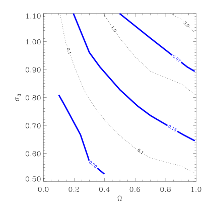
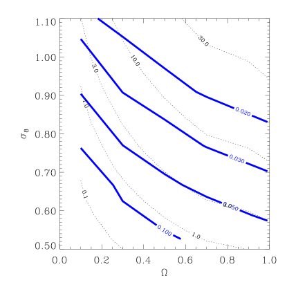
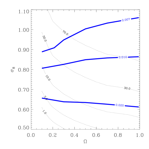
Figure 3: Contours of the SZ angular correlation function are shown as solid lines in the $(\sigma_{8},\Omega_{\rm M})$–plane for different limiting flux values: top left, $Y_{\rm lim}=10^{-3}$ arcmin²; top right, $Y_{\rm lim}=10^{-4}$ arcmin²; and bottom left, $Y_{\rm lim}=10^{-5}$ arcmin². The Hubble constant is fixed at $h=0.7$. Each contour is labeled with the value of the correlation function at a separation of $\theta=30$ arcmins. Contours of the SZ cluster counts at the same flux limits are shown as the dotted lines, and labeled in units of 1/sq.deg. The SZ flux normalization $Y_{*}=7.6\times 10^{-5}h^{7/6}$ arcmin² .

Figure 4: Effect of varying $Y_{*}$. The contours have the same meaning as in the previous figure, and $h=0.7$ as before. All three panels correspond to a flux limit of $Y_{\rm lim}=10^{-4}$ arcmin², but $Y_{*}$ changes from $3.8\times 10^{-5}h^{7/6}$ arcmin² (upper left) to $7.6\times 10^{-5}h^{7/6}$ arcmin² (upper right; same as upper right panel of previous figure) and finally $1.5\times 10^{-4}h^{7/6}$ arcmin² (lower left). The contours and their spacing are stretched upward as $Y_{*}$ decreases. The intersection points of the two sets of contours essentially move vertically, changing in $\sigma_{8}$ and remaining roughly fixed in $\Omega_{\rm M}$.

4.3 Influence of the ICM

The single relation Eq. (6) incorporates all of the ICM physics, and from the nature of the SZ flux, we expect it to be rather tight with little scatter. There is virtually no direct observational information on this relation, while numerical simulations (da Silva et al. 2003) do indeed confirm a small scatter. They also indicate that there is only a slight deviation from the self–similarity with $\alpha=0.1-0.2$ and $\gamma=0$ down to masses well below $10^{14}\;$M_⊙. X–ray observations, on the other hand, demonstrate deviations from self–similarity. This is most clear for low–mass systems with temperatures below $T\sim 2$ keV, but even in the richer systems the observed $L$–$T$ deviates from the self–similar expectation. These results are beginning to be reproduced by numerical simulations including cooling/heating (e.g., Borgani et al. 2002), including those that indicate only slight deviation from self–similarity for the SZ relation Eq. (6) (Muanwong et al. 2002). That X–ray observables show greater deviation from self–similarity than the SZ flux is not surprising, given that the former are more sensitive to spatial/temperature structure in the gas than the latter, as emphasized previously. This is precisely the advantage of SZ surveys.

As mentioned, low mass systems with the greatest deviation from self–similarity in X–rays contribute little to counts and the angular function at a flux limit of $Y_{\rm lim}=10^{-4}$ arcmin². For example, for $\Omega_{\rm M}<0.6$ and values of $\sigma_{8}$ in the range 0.6–1, the uncertainty on $\sigma_{8}$ due to the presence of low mass systems with $T<2$ keV is around $5\%$, well within our estimated errors on the angular correlation function (Eq. 8 below). We therefore focus on the effects of changing the normalization, Eq. (7), of the self–similar SZ flux–Mass relation ($\alpha=\gamma=0$). Physically, this represents an uncertainty in the average thermal gas energy of galaxy clusters. Figure 4 shows the effect of changing $Y_{*}$ at a flux limit of $Y_{\rm lim}=10^{-4}$ arcmin². From the figure, we see that changing this normalization stretches the counts and angular function contours vertically by roughly the same amount, their point of intersection (if any) remaining at roughly the same value of $\Omega_{\rm M}$. For example, a factor 2 change in normalization moves the intersection by $\sim 10-20$ % in $\sigma_{8}$ (e.g., at $\Omega_{\rm M}\sim 0.3$). This represents an inherent systematic caused by modeling uncertainty associated with the ICM. Uncertainties related to ICM modeling have been extensively discussed by Moscardini et al. (2002) for the full 3D spatial correlation function of SZ clusters.
Including the uncertain SZ flux normalization, $Y_{*}$, we now have three parameters to determine, and so additional information is needed; for example, an observational program to determine the $Y$–$M$ relation on a representative sample of clusters. Another tactic is to use the constraint arising from the local cluster abundance as measured by the X–ray temperature function.

4.3.1 Adding the local cluster abundance constraint

For a fixed value of $T_{*}$, the local X–ray temperature function constrains the cosmological parameters $\sigma_{8}$ and $\Omega_{\rm M}$ to a well–defined curve in the plane: $\sigma_{8}\Omega_{\rm M}^{0.6}\approx 0.6T_{*}^{-0.8}$ (Pierpaoli et al. 2002). The exact relation depends somewhat on the chosen mass function. Consider such a constraint, shown as the middle dashed line in Figure 5. Supposing that we measure now both the SZ counts and angular function, finding 7.7 $\leavevmode\nobreak\ sq.\leavevmode\nobreak\ deg$ and $w(\theta=30\;{\rm arcmins})=0.024$, respectively, at $Y=10^{-4}$ arcmin² and given as the solid contours in the figure. Apart from the cosmological parameters $\sigma_{8}$ and $\Omega_{\rm M}$, the SZ contours depend only on $Y_{*}$, whose value is uncertain; by changing $Y_{*}$, we move the SZ contours around the plane, as previously described. However, there is a unique value for $Y_{*}$ that reduces the intersection of the three lines to a single point in the plane. By adjusting $Y_{*}$ to this value, we simultaneously constrain the cosmological parameters and the normalization $Y_{*}$. In the figure, this intersection lies on top of the true underlying model. The determined value of $Y_{*}$ together with the known $T_{*}$ imply a constraint on $f_{\rm gas}$. By adding the information on the local cluster abundance, we have pinned down the relevant ICM physics and constrained the cosmological parameters, eliminating the primary uncertainty in using SZ clustering observations (Moscardini et al. 2002). Unfortunately, $T_{*}$ is at present only poorly known, with simulations and observations indicating values generally in the range $1.2-2$ (Pierpaoli et al. 2002; Muanwong et al. 2002; Huterer $\&$ White 2002). We expect that it will be much better determined by the time large SZ catalogs become available, making this kind of analysis possible.

This example illustrates the utility of the angular function: with only the local cluster abundance and the SZ counts, we cannot determine the cosmological parameters $\sigma_{8}$ and $\Omega_{\rm M}$, due to the uncertainty on $Y_{*}$. Adding the angular function breaks the degeneracy. We are thus able to constrain the cosmology with the 2D SZ catalog, without recourse to redshift determinations. Constraints obtained in this way are particularly useful for their complementarity to constraints from CMB anisotropy and distance measurements with SNIa. For example, with SZ clusters we measure $\sigma_{8}$ directly on the relevant scales and constrain $\Omega_{\rm M}$, as opposed to the physical density $\Omega_{\rm M}h^{2}$ in the case of the CMB.

Figure 5: Example of constraints in flat models. The true underlying model corresponds to $\Omega_{\rm M}=0.3$, $\sigma_{8}=0.9$, $f_{\rm gas}=0.07/h^{1.5}$ and $T_{*}=1.5$ keV, corresponding to $Y_{*}=1.1\times 10^{-4}h^{7/6}$ arcmin². For this model, one would observe 7.7 clusters/sq.deg. for the counts and $w=0.024$ for the angular function at 30 arcmins, respectively, both at a flux limit of $Y=10^{-4}$ arcmin². The bold (heavy blue) line shows the constant counts contour in the plane, while the thin (lighter blue) line indicates the angular function contour at the observed value. The middle dashed line represents the constraint from the local X–ray cluster temperature function, for the true value of $T_{*}$; the other two dashed lines correspond to the constraints for $T_{*}=2$ keV (bottom dashed curve) and $T_{*}=1$ keV (upper dashed curve). The three sets of contours cross at a unique point. The gray shaded band indicates the estimated statistical uncertainty on $w$ attainable with the Planck survey (the error on the counts is roughly the thickness of the contour).

As mentioned above, clusters below $\sim 2$ keV contribute little to the contours at our fiducial flux limit of $Y=10^{-4}$ arcmin². At lower flux limits, more representative of future ground–based surveys, we could expect that the possible effects of deviations from self–similar scaling become more important, although simulations at present indicate only mild effects on the SZ flux.

4.4 Discussion of statistical errors

Before concluding, we briefly examine the statistical errors expected on a measurement of the SZ angular correlation function. Although a thorough analysis of this issue requires detailed simulations of a given survey, we may nonetheless make some general arguments to gain insight into what may eventually be achieved. We take the Planck survey as our example. The resolution of the Planck SZ catalog will be on the order of 5 arcmins (at best), so we can only expect to measure the correlations on larger scales (as the $30\arcmin$ we have chosen in our analysis), and the fiducial sensitivity expected is $Y\sim 10^{-4}$ arcmin² (Aghanim et al. 1997; Bartelmann 2001). Since the angular correlations are small in this context ($\leq 0.1$), we may estimate the (statistical) error on a measurement of $w(\theta)$ as the Poisson variance in the number of pairs, $n_{\rm pair}$, at this separation (e.g., Peebles 1980; Landy & Szalay 1993). This quantity is determined by the counts as follows: Suppose that we measure $w$ in a annular bin of width $\Delta\theta$ at angular distance $\theta$ from a cluster. The mean number of clusters in this ring is $\langle n\rangle=2\pi\theta\Delta\theta\Sigma(Y_{\rm lim})$, from which we deduce that the total number of pairs at this separation in a catalog of $N$ clusters is about $n_{\rm pair}\approx(1/2)N\times\langle n\rangle=N\pi\theta\Delta\theta\Sigma$. In other words, we estimate the error to be

$$\Delta w(\theta,Y_{\rm lim}) \approx\frac{1}{2\pi}\left[\Sigma(Y_{\rm lim})\right]^{-1}\frac{1}{\theta}\left(\frac{\Delta\theta}{\theta}\right)^{-1/2}$$ (8)

$$\approx 2.78\times 10^{-3}\left(\frac{{\rm deg}}{\theta}\right)\left(\frac{\Delta\theta}{\theta}\right)^{-1/2}\left(\frac{\Sigma}{{\rm deg}^{2}}\right)^{-1}$$

Notice that this statistical error depends essentially on the number counts $\Sigma$. This leads to the gray shaded area in Figure 5

5 Discussion and Conclusion

We have calculated the angular correlation function of SZ–detected clusters in order to evaluate its usefulness for extracting cosmological information directly from a 2D SZ cluster survey, before 3D follow–up. The angular correlation function of SZ detected clusters differs from the angular power spectrum of SZ induced CMB anisotropies, which is dominated by the Poisson term. The different scaling of angular correlations with survey depth visually demonstrates the cosmological sensitivity of the angular function (See Figs 1, 2). As illustration, we considered the parameter pair $(\Omega_{\rm M},\sigma_{8})$ in the context of flat $\Lambda$–CDM models. We found that at sufficient depth (e.g., $Y_{\rm lim}\sim 10^{-4}$ arcmin², comparable to the Planck mission), the counts and angular function combined can constrain these parameters. Modeling uncertainty associated with the ICM may be reduced by measuring the $T$–$M$ relation and adding the corresponding constraint from the local abundance of X–ray clusters; in this way, the two cosmological parameters and the SZ flux normalization $Y_{*}$ may be found. Deeper ground–based surveys (e.g., $Y_{\rm lim}\sim 10^{-5}$ arcmin²), will pick up a larger number of low–mass objects whose ICM properties require more careful modeling of deviations from self–similarity.

The accuracy and precision with which one will be able to measure the angular function (and the counts) is clearly an important issue. We only briefly touched on this point with a simple estimate of the expected statistical errors expected on $w(\theta)$ in the case of the Planck mission. A more detailed examination incorporating simulations of the SZ survey characteristics, including instrument noise and foreground contamination, as well as of the catalog extraction algorithms, is needed. The survey selection function will in reality depend on these details (Bartlett 2001; Melin et al. 2003; White 2003), and so will the errors on the counts and measured angular function.

It is clear that the most powerful constraints from an SZ survey will come from its measured redshift distribution. The interesting point is, however, that the method proposed here increases the immediate scientific return from an SZ survey by offering a way to obtain pertinent cosmological constraints using only a 2D SZ catalog, without recourse to follow–up observations.