Variability of sub-mJy radio sources

Abstract

We present 1.4 GHz VLA observations of the variability of radio sources in the Lockman Hole region at the level of $\geq 100\mu$Jy on timescales of 17 months and 19 days. These data indicate that the areal density of highly variable sources at this level is $<5\times 10^{-3}$ arcmin^-2. We set an upper limit of $2\%$ to the fraction of 50 to 100$\mu$Jy sources that are highly variable ($\rm\Delta S\geq 50\%$). These results imply a lower limit to the beaming angle for GRBs of 1^o, and give a lower limit of 200 arcmin² to the area that can be safely searched for GRB radio afterglows before confusion might become an issue.

1 Introduction

Synoptic surveys for Gamma-ray bursts (GRBs), and subsequent ground-based observational follow-up at radio through optical wavelengths, has highlighted the importance of transient celestial phenomena (Masetti 2001). The new parameter space of the transient cosmos has been emphasized in the design of future telescopes, such as the optical Large Synoptic Survey Telescope (Tyson & Angel 2001), and the radio Square Kilometer Array (van Haarlem 1999).

While it is well documented that flat spectrum radio sources can be variable (Aller et al. 1985), the areal density of such sources has not been well quantified through multi-epoch, wide field blind surveys. At high flux density levels ($>10$ mJy at 1.4 GHz), one can make a rough estimate of the areal density of variable radio sources by simply assuming that all flat spectrum sources are variable. For instance, the areal density of all sources $\geq 10$mJy is $\sim 2\times 10^{-3}$ arcmin^-2, and the fraction of flat spectrum sources is about 10$\%$, implying an areal density of variable radio sources of $\sim 2\times 10^{-4}$ arcmin^-2 (Gruppioni et al. 1999; White et al. 1997; Windhorst et al. 1985; Hopkins et al. 2000, 2002). This number is consistent with the (null) results of Frail et al. (1994) in their search for highly variable mJy-level sources associated with GRBs.

Source populations at these high flux densities are dominated by AGN. Below about 1 mJy the slope of the source counts flattens, and star forming galaxies are thought to dominate the faint source population (Windhorst et al. 1985; Georgakakis et al. 1999; Hopkins et al. 2000, 2002). Hence, when considering the areal density of variable sub-mJy radio sources, one cannot simply extrapolate the results from high flux density source samples to low flux densities.

Knowledge of the areal density of variable sub-mJy radio sources is critical for setting the back-ground, or ‘confusion’, level for studies of faint variable source populations, such as GRBs (Frail et al. 1997). A recent comparison of the NVSS and FIRST surveys by Levinson et al. (2002) sets a conservative upper limit of $3\times 10^{-6}$ arcmin^-2 to the areal density of ‘orphan’ GRB radio afterglows (i.e. GRBs for which the $\gamma$-ray emission is not beamed toward us) with S${}_{1.4}\geq 6$ mJy. They also argue that the areal density of radio supernovae will be considerably smaller. While the area of the sky covered by Levinson et al. (2002) was much larger that the study presented herein, their flux density limit was higher than any GRB radio afterglow yet recorded. In this paper we present a smaller area study, but we consider variable sources at flux density levels ($\sim 0.1$mJy) applicable to typical GRB radio afterglows.

In general, variability of radio sources at the sub-mJy level is an essentially unexplored part of parameter space – a part of parameter space which may fundamentally drive the design of future radio telescopes, such as the SKA (Carilli et al. 2002). Herein we present the first study to delve into this part of parameter space, by exploring systematically the variability of the sub-mJy radio source population at 1.4 GHz. We examine variability on timescales of 17 months and 19 days. Note that the LSST will probe similar variability timescales in the optical, with sampling on weekly to yearly timescales.

2 Observations

Observations were made using the using the VLA at 1.4 GHz in the B configuration (maximum baseline = 10km). The region observed is in the Lockman Hole centered at: (J2000) 10^h 52^m 56.00^s, 57^d 29^′ 06.0^′′. Table 1 summarizes the observations. Column 1 gives the observing date, column 2 gives the observed hour angle range, and column 3 gives the rms in the final image. These observations are part of a larger multiwavelength program to study the evolution of dusty star forming galaxies (Bertoldi et al. in prep).

Standard wide field imaging techniques were employed in order to generate an unaberrated image of the full primary beam of the VLA (FWHM = 32^′). The absolute flux density scale was set using 3C286. We then generated a CLEAN component model of the field using self-calibrated data taken on Sept. 5, 2002. The data from all days were then self-calibrated in amplitude and phase without gain renormalization using this model. This process should ensure that all the data are on the same flux scale. Images made before and after this process showed that the absolute flux scale changed by at most 1$\%$. We also checked to see if variable sources could be removed (or added) due to using a single model to self-calibrate data from all the different days. Components at the 0.1 to 0.2 mJy level were added to the self-calibration model at random positions in the field, and the self-calibration process was repeated. In no case was a new source generated. This gives us confidence that the self-calibration process is robust to small perturbations in the model, i.e. that the problem is over-constrained and that the input self-calibration model is dominated by non-varying sources.

Images for each day were generated using the wide field imaging capabilities in the AIPS task IMAGR (Perley 1999). To remove problems with ‘beam squint’ (slightly different pointing centers for right and left circular polarizations) the right and left polarizations were imaged separately. The images were then summed, weighted by the rms on each image. The final image using data from all the observing days is shown in Figure 1. The rms noise on this image is 7$\mu$Jy beam^-1 and the restoring CLEAN beam is circular with FWHM = 4.5^′′.

3 Analysis

We searched for source variations over 17 months by comparing images made in April 2001 with those made in August/September 2002, and also on timescales of 19 days by comparing images made on August 17 and September 5, 2002. We searched for variable sources out to the 10$\%$ point of the primary beam, and we limited the analysis to sources with variations $>2\%$. Images from all epochs were convolved to 6^′′ resolution to mitigate differences that might occur due to the non-linear process of deconvolution. The rms on the images used for variability analysis was 12.5 $\mu$Jy for the 17 month comparison, and 17$\mu$Jy for the 19 day comparison.

The images from different epochs were both subtracted and averaged. A fractional variability image was then generated by dividing these two images, blanking at the 5$\sigma$ level (in absolute value). For the 17 months variability analysis $\sigma$ was 17$\mu$Jy on the differenced image, and 9$\mu$Jy on the averaged image. The corresponding numbers for the 19 day analysis were 26$\mu$Jy and 15$\mu$Jy, respectively.

The difference image for the 17 month analysis is shown in Figure 2. Some artifacts are seen around the brighter extended sources arising from differences in deconvolution and residual calibration errors. Beyond these artifacts, the difference images are remarkably free of sources. This result gives us confidence that the imaging process (self-calibration and deconvolution) does not generate spurious sources at the $\geq 5\sigma$ level, and tells us right away that the radio sky is not highly variable at the 100$\mu$Jy level.

Variable sources were identified in the divided image. Five variable sources were found at the $5\sigma$ level in the 17 month comparison, while four sources were found in the 19 day analysis. We then returned to the original images to find the flux densities of the sources at each epoch. Table 2 lists source positions (columns 1 and 2), flux densities at the two epochs (columns 3 and 4), and the distance from the phase center (column 5) for the 17 month analysis, and Table 3 lists the corresponding values for the 19 day analysis. Note that the source J1051+5734 was seen to vary on both timescales. In fact, this source varied between September 5 and September 9 from 1.53 mJy to 0.71 mJy. The September 2002 value listed in Table 2 is the weighted average of these two measurements.

We next consider the sensitivity of our observations to variable sources at some absolute level, $\Delta$S. The analysis is complicated by the roughly Gaussian roll-off of the primary beam of the VLA, with FWHM $\sim 32^{\prime}$. Identification of variable sources was done using the non-primary beam corrected maps in order to have uniform noise across the field. Of course, the final flux densities and noise levels for the variable sources were corrected for the primary beam attenuation.

Given a $\Delta$S, one can calculate the maximum primary beam correction, f, for which a change in flux density $\Delta$S could be detected at the 5$\sigma$ level, where $\sigma$ is the noise at the field center on the difference image: f = 5$\sigma$/$\Delta$S. The value of f then sets the distance from the pointing center, R, to which such variation could have been detected, given the primary beam shape of the VLA.

Values for $\Delta$S, f, and R are listed in columns 1, 2, and 3, respectively in Table 4. Column 4 lists the number of variable sources over 17 months that meet these criteria. Column 5 lists the number of sources within the specified radius with flux density, S $\geq$ $\Delta$S/2. This flux density sets the limit for 100$\%$ variability, e.g. a source could be 100$\mu$Jy on day 1, and 0 $\mu$Jy on day 2, leading to a value on the difference image of 100 $\mu$Jy and a value on the average image of 50$\mu$Jy. Column 6 lists the areal density of sources with S$\geq$$\Delta$S/2 on our Lockman hole image, while column 7 lists the corresponding values from the recent study of Fomalont et al. (2002) comprised of a number of different fields.

We have investigated the source sizes using the B array observations at 4.5^′′ resolution. Two of the sources are partially resolved. For J1051+5708 Gaussian fitting to the profile yields a peak surface brightness, I${}_{\nu}=8.92\pm 0.05$ mJy beam^-1, a total flux density, S${}_{\nu}=10.00\pm 0.09$ mJy, and a (deconvolved) size of $1.9^{\prime\prime}\times 1.1^{\prime\prime}$, with major axis position angle (PA) = $37^{o}$. The corresponding numbers for J1055+5718 are: I${}_{\nu}=8.82\pm 0.06$ mJy beam^-1, S${}_{\nu}=12.35\pm 0.13$ mJy, and $3.4^{\prime\prime}\times 2.2^{\prime\prime}$ at PA $=81^{o}$. The rest of the sources are unresolved, with upper limits between 1^′′ and 2^′′ depending on signal-to-noise.

The nature of this analysis is such that we are not sensitive to very rapid variations, e.g. timescales of minutes or less. For instance, a 50 mJy flare of 1 min duration would average down to about 100$\mu$Jy over 7 hours. While our nominal sensitivity would be adequate to detect such an event, the existence of such a transient source in the visibility data would lead to errors in the self-calibration and imaging process which would manifest themselves clearly on the images. Of course, it is possible that such a bright, short timescale event was mis-identified as interference in the data editing process, and removed.

4 Discussion

For the analysis on 17 month timescales we could have detected sources with $\Delta$S $\geq 100\mu$Jy out to a radius of 7.8^′, but none were detected. This sets an upper limit to the areal density of such sources of $5\times 10^{-3}$ arcmin^-2. Another interesting point is that within this radius there are 46 sources between 50 and 100 $\mu$Jy on the averaged image. Hence, we set an upper limit of about 2$\%$ to the fraction of sources in this flux density regime that are highly ($\geq 50\%$) variable.

These results are grossly consistent with the idea that below 1 mJy at 1.4 GHz the radio source population is dominated by star forming galaxies, as compared to AGN which dominate at high flux densities (Hopkins 2000, 2002). The exact distribution of AGN vs. starbursts vs. other source types as a function of radio flux density is not fully determined at this time, and is an area of active current research (Hopkins et al. 2002; Georgakakis et al. 1999; Richards 2001; Fomalont et al. 2002). As a rough guide we consider the models of Hopkins et al. (2000). They suggests that at $\geq$ 10 mJy the source population is 90$\%$ steep spectrum radio sources, 10$\%$ flat spectrum radio sources, and $\leq 1\%$ star forming galaxies. Again, at high flux density levels the flat spectrum sources correspond to the variable radio source population. At 100 $\mu$Jy the models suggests that the proportions change to roughly 80$\%$ star forming galaxies, 15$\%$ steep spectrum AGN, and 5$\%$ flat spectrum AGN.

These models have not considered truly transient source populations, such as GRB radio afterglows, which have timescales of 10’s of days. The statistics of radio afterglows of GRBs are such that in an area of 7.8^′ radius one would expect to see $\sim 0.005$ sources above 0.1 mJy at 1.4 GHz at any given time, assuming GRBs are highly beamed (see below). Hence, the fact that we did not see such a source is not surprising. More importantly, the results presented herein allow us to set a limit on the variable source confusion level for GRB radio afterglow searches, again at a flux density level relevant to the observed population. For example, radio searches are needed for localizing an important subclass of afterglows known as ‘dark GRBs’ (e.g., Djorgovski et al. 2001), for which optical emission from the GRB is not detected. It has been suggested that the absence of optical emission from these sources is the result of either dust obscuration, or the Gunn-Peterson effect, i.e. Ly$\alpha$ absorption by the neutral intergalactic medium. This latter effect would place the sources at $z>6.3$ (Fan et al. 2003). An upper limit to the areal density of $5\times 10^{-3}$ arcmin^-2 for variable sources at the 100$\mu$Jy level implies a lower limit of 200 arcmin² to the area that can be safely searched at 1.4 GHz before one such source is expected to be detected by chance. For comparison, the typical GRB error circle is $\sim$30 arcmin², but larger error circles are not uncommon.

This result can also be used to derive a rough limit on the mean beaming angle for GRBs (Perna & Loeb 1998). From a sample of 25 radio afterglows (Frail et al. in prep) we estimate that 10-25% will be visible above the 100 $\mu$Jy level at 1.4 GHz, with an average lifetime of one month. The GRB event rate is approximately 600 per year (Fishman & Meegan 1995) so we expect to find only $8.4\times 10^{-8}$ arcmin^-2. However, if GRBs are highly beamed, as recent studies seem to suggest (Frail et al. 2001), then our upper limit to areal density of $5\times 10^{-3}$ arcmin^-2 implies a beaming factor $f_{b}<6\times 10^{4}$, or a mean jet opening angle $\theta_{j}>1^{\circ}$. This value is not very constraining compared to existing limits, but to our knowledge this is the first time a survey for variability has been done at the appropriate flux level for radio afterglows. More stringent limits will require sensitive, larger area surveys with existing or planned instruments (Totani & Panaitescu 2002).

A final point we consider is cosmic variance. It is possible that the Lockman hole region we have sampled was just statistically-poor in transient sources. A rough indication of the effect of cosmic variance comes from the overall source counts (columns 6,7 in Table 4). The source counts we derive agree to within 20$\%$ with those found by Fomalont et al. (2002) in other areas of the sky. In general, it has been found that for 30^′ fields-of-view the maximum field-to-field scatter in the sub-mJy source counts is about a factor two (Fomalont et al. 2002). We consider this an upper limit to the effect cosmic variance has on the areal density of variable source presented herein.

The National Radio Astronomy Observatory (NRAO) is operated by Associated Universities, Inc. under a cooperative agreement with the National Science Foundation. We thank F. Owen, E. Fomalont, R. Becker, and J. Condon for useful comments concerning this work, and the referee for careful and insightful criticism.

Table 1: Observations

Date	Hour Angle Range	RMS
		$\mu$Jy
April 22, 2001	-4.2 to +1.0	15
April 27, 2001	-4.2 to +1.3	15
August 17, 2002	-2.2 to +3.4	17
September 5, 2002	-3.2 to +3.7	16
September 9, 2002	-2.8 to +3.1	18

Table 2: Variable sources: April 2001 to Sept 2002

RA	Dec	IApril2001	ISept2002	Radius
J2000	J2000	mJy beam-1	mJy beam-1	arcmin
10 50 39.53	57 23 36.5	$5.70\pm 0.036$	$4.48\pm 0.036$	19.2
10 51 22.06	57 08 54.8	$9.47\pm 0.07$	$9.98\pm 0.07$	23.8
10 51 42.03	57 34 47.7	$0.80\pm 0.018$	$1.18\pm 0.018$	11.4
10 54 00.48	57 33 21.2	$2.79\pm 0.016$	$2.66\pm 0.016$	9.7
10 55 48.52	57 18 27.5	$10.96\pm 0.10$	$10.08\pm 0.10$	25.6

Table 3: Variable sources: August 17 to Sept 5, 2002

RA	Dec	I${}_{\rm Aug~{}17}$	I${}_{\rm Sept~{}5}$	Radius
J2000	J2000	mJy beam-1	mJy beam-1	arcmin
10 51 38.08	57 49 56.5	$1.97\pm 0.099$	$3.02\pm 0.099$	23.3
10 51 42.03	57 34 47.7	$1.22\pm 0.027$	$1.53\pm 0.027$	11.4
10 52 06.44	57 41 09.7	$9.24\pm 0.031$	$9.58\pm 0.031$	13.8
10 52 25.39	57 55 05.6	$23.4\pm 0.18$	$25.4\pm 0.18$	26.3

Table 4: Search radius for variable sources at 1.4 GHz

$\Delta$S	fa	Rb	N${}_{\rm var}^{c}$	N${}_{\rm srcs}^{d}$	Nsrcs/areae	Nsrcs/areaf
mJy		arcmin		$\rm S\geq\Delta S/2$	$\rm S\geq\Delta S/2$ arcmin-2	$\rm S\geq\Delta S/2$ arcmin-2
0.13	0.65	12.7	1	219	0.43	0.53
0.3	0.28	20.9	1	222	0.16	0.21
0.50	0.17	23.9	1	187	0.10	0.12
0.85	0.1	27.0	1	139	0.061	0.067

^af = 5$\sigma/\Delta$S, where $\sigma=17\mu$Jy = rms on difference maps at the field center.

^bR = distance from pointing center out to which $\Delta$S can be detected to $\geq 5\sigma$.

^cN_var = number of variable sources $\geq\Delta$S within given radius over 17 months.

^dN_srcs = number of sources with flux density, $\rm S\geq\Delta S/2$ within R. This S sets the 100$\%$ variability detection limit.

^eN_srcs/area = number of sources with $\rm S\geq\Delta S/2$ per arcmin² from our Lockman Hole field.

^fN_srcs/area = number of sources with $\rm S\geq\Delta S/2$ per arcmin² from the study of Fomalont et al. (2002): N($\rm\geq S_{mJy})=0.026\times S^{-1.1}~{}arcmin^{-2}$.

Figure Captions

FIG. 1.— Radio image of the Lockman Hole at 1.4 GHz with a resolution of 4.5^′′. The rms noise on the image is 7$\mu$Jy. The grayscale range is from -0.15 mJy to 0.25 mJy.

FIG. 2.— The difference image between observations in April 2001 and Aug/Sept 2002 at 6^′′ resolution. The grayscale range is from -0.2 mJy to 0.2 mJy.

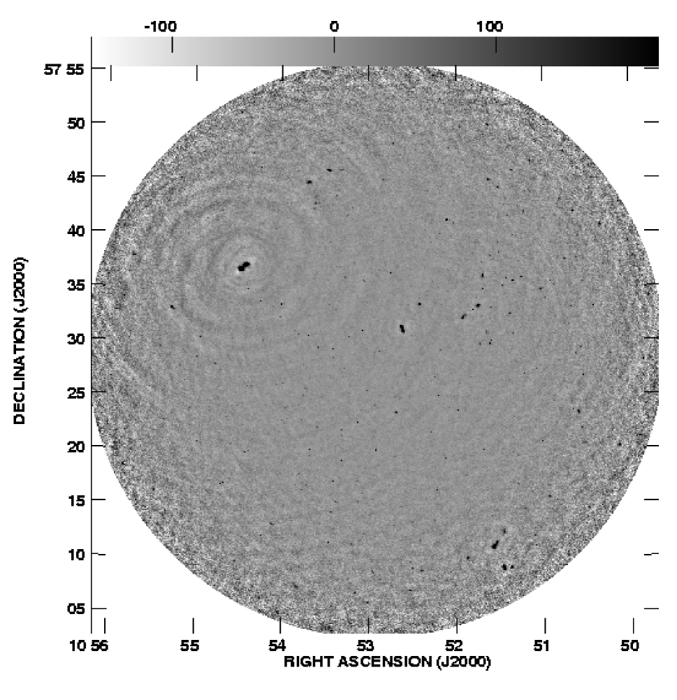
Figure 1:

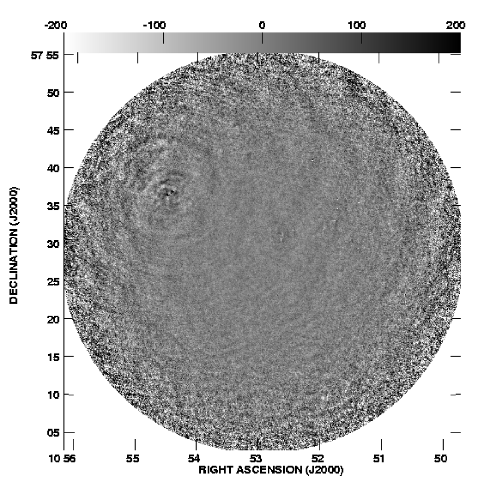
Figure 2: