Surprisingly Little O VI  Emission Arises in the Local Bubble

Abstract

This paper reports the first study of the O VI resonance line emission ($\lambda\lambda$ 1032, 1038) originating in the Local Bubble (or Local Hot Bubble) surrounding the solar neighborhood. In spite of the fact that O VI absorption within the Local Bubble has been observed, no resonance line emission was detected during our 230 ksec Far Ultraviolet Spectroscopic Explorer observation of a “shadowing” filament in the southern Galactic hemisphere. As a result, tight 2 sigma upper limits are set on the intensities in the 1032 and 1038 Å emission lines: 500 and 530 photons cm^-2 s^-1 sr^-1, respectively. These values place strict constraints on models and simulations. They suggest that the O VI-bearing plasma and the X-ray emissive plasma reside in distinct regions of the Local Bubble and are not mixed in a single plasma, whether in equilibrium with $T\sim 10^{6}$ K or highly overionized with $T\sim 4$ to $6\times 10^{4}$ K. If the line of sight intersects multiple cool clouds within the Local Bubble, then the results also suggest that the hot/cool transition zones differ from those in current simulations. With these intensity upper limits, we establish limits on the electron density, thermal pressure, pathlength, and cooling timescale of the O VI-bearing plasma in the Local Bubble. Furthermore, the intensity of O VI resonance line doublet photons originating in the Galactic thick disk and halo is determined (3500 to 4300 photons cm^-2 s^-1 sr^-1), and the electron density, thermal pressure, pathlength, and cooling timescale of its O VI-bearing plasma are calculated. The pressure in the Galactic halo’s O VI-bearing plasma (3100 to 3800 K cm^-3) agrees with model predictions for the total pressure in the thick disk/lower halo. We also report the results of searches for the emission signatures of interstellar C I, C II, C III, N I, N II, N III, Mg II, Si II, S II, S III, S IV, S VI, Fe II, and Fe III.

1 Introduction

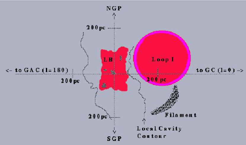
Figure 1: The Local Bubble (LB) is sketched in red in the center of the cartoon. The LB’s size and shape were drawn from Snowden et al. (1998). The gray spots within the LB represent the cool clouds. The dotted, wiggly lines beyond the Local Bubble depict the outline of the Local Cavity, whose shape and size has been taken from the 50 mÅ Na I D2 projected contours in Sfeir et al. (1999). To the right and lower right of the LB are cartoons representing the nearby Loop I superubble and the observed filament. Note that the filament is well beyond the calculated extent of the Local Bubble. An axis has been superimposed. The Sun lies at the origin. The Galactic center (GC) is to the right, the Galactic anticenter (GAC) is to the left, the north Galactic pole (NGP) is at the top, and the South Galactic pole (SGP) is at the bottom. Each of the tick marks is 200 pc from the center of the grid.

The Local Bubble (LB) or Local Hot Bubble and its environment are sketched in Figure 1. The Local Bubble, a $\sim 10^{6}$ pc³ region of X-ray emissive, presumably hot ($\sim 10^{6}$ K) plasma, is nestled within a rarefied cavity in the Galactic disk called the Local Cavity, (Knapp, 1975; McCammon et al., 1983; Snowden et al., 1998; Sfeir et al., 1999). Within the Local Bubble, lie a number of cool ($\sim 10^{4}$ K) clouds, including the complex of parsec-scale clouds surrounding the Sun (Frisch, 1986; Lallement & Bertin, 1992; Gry et al., 1995). Estimates of the number of clouds per line of sight range from $\sim 2$ to $\sim 6$, with $\sim 2$ coming from the ratio of the typical observed absorbing column density (Hutchinson et al., 1998) to the absorbing column density of the local cloud (Lallement et al., 1995), and $\sim 6$ coming from the number of clouds along the $\epsilon$ CMa line of sight (Gry et al., 1995). Beyond the Local Bubble, in the direction of the Galactic center, lies a superbubble named Loop I, which was blown by the stars and supernovae in the Sco Cen association (Egger, 1993).

The Local Bubble is larger and more energetic than a supernova remnant, yet smaller and less energetic than a superbubble. Such bubbles are important as most of the hot gas in the Galactic disk resides within them. Like the distribution of small versus large stellar associations, the population of bubbles is likely to be larger than the population of superbubbles. Nonetheless, because its softer X-ray photons from its relatively cooler plasma are more easily absorbed, a bubble like the Local Bubble would be much more difficult to detect from a great distance than would an energetic superbubble like Loop I. Thus, many other Local Bubble analogs may reside within the Galaxy, unknown to us because they are obscured by the neutral and molecular material of the Galactic disk. In this sense, we are fortunate to have a local specimen to examine.

At this time, our understanding of the Local Bubble is chiefly phenomenological. To some degree, the Local Bubble is defined as the source of soft X-rays ($\sim\frac{1}{4}$ keV) produced between us and the nearest opaque material. Its physical presence has been surmised from the anti-correlation between soft X-ray intensities and neutral hydrogen column densities (associated with the larger Local Cavity), detections of X-rays originating in the foreground of opaque clouds, relative constancies between Be (0.07 to 0.11 keV), B (0.13 to 0.19 keV) and C (0.16 to 0.28 keV) band surface brightnesses across the sky (implying very little absorption as the effective absorption cross sections vary significantly between the bands), and consistency among two decades of X-ray observations.

Fundamental characteristics of the LB, such as its presumed temperature and size, cannot be determined directly, but can only be estimated when additional constraints (such as ionizational equilibrium, constancy of emissivity, and filling factor) are assumed. Given these assumptions, the estimated temperature has been derived from the ratio of fluxes in broad soft X-ray bands. In directions where the Galactic disk blocks all of the $\frac{1}{4}$ keV emission from beyond the Local Bubble, the observed ROSAT R2 to R1 band ratio is $\sim 1.06$, implying a temperature of $10^{6.1}$ K (Kuntz & Snowden, 2000). This temperature is consistent with values found by shadowing observations (described below) at higher Galactic latitudes (Kuntz & Snowden, 2000; Snowden et al., 2000) and with Wisconsin’s Ultrasoft X-ray Telescope (UXT) and All-Sky Survey’s B/Be and C/B band ratios (Bloch et al., 1986; Juda et al., 1991). Similar temperatures were also derived from the Diffuse X-ray Spectrometer’s soft X-ray spectra, although these high resolution spectra were difficult to fit with simple models (Sanders et al., 2001).

Desirous of a better understanding of our environs as well as a model of the bubble population (useful for calculating the hot gas filling factor), both observers and theorists have long sought explanations of the LB’s origin and life history. Many researchers have pointed out that the energy embodied in the Local Bubble’s X-ray emitting plasma is so great as to require a supernova or a series of supernovae, possibly aided by stellar winds. The energy may have been deposited within an existing gap in the H I disk or may have pushed aside the disk material to create a cavity. Alternatively, the explosion(s) and winds may have originated in the nearby Loop I (Sco-Cen) superbubble and blown into the solar region (Frisch, 1981; Bochkarev, 1987), or the Local Bubble and Loop I may have been blown independently but are now interacting (Egger & Aschenbach, 1995). In some of these scenarios, the X-ray emitting plasma may have expanded after being shock heated, vastly cooling the plasma, retarding the collisional recombination rates, and thus “freezing” the plasma into an “overionized” state (Breitschwerdt & Schmutzler, 1994; Breitschwerdt, 2001). In contrast, if the expansion was restrained and the time-scale was long, the plasma may have already approached collisional ionizational equilibrium (Smith & Cox, 2001). These two cases should produce markedly different spectral signatures. Presently, many theorists and observers are working to decipher the Local Bubble’s life story by comparing its X-ray spectra to spectra predicted by hydrodynamical simulations. It is hoped that when the observed fluxes in multiple bands or emission lines are matched by the predictions of a particular type of model, then we will have found a key to deciphering the story of the Local Bubble. Here, we extend this sort of comparison into the ultraviolet, using the O VI resonance line (1032, 1038 Å) intensities. We also compare the intensities with O VI absorption line column densities taken from the literature, in order to estimate the physical properties of the O VI-bearing plasma.

We use the “shadowing” strategy long employed in X-ray analyses to isolate the Local Bubble’s emission from the more distant interstellar medium’s emission (see Section 2). The observations (228 ksec toward $l=278.6^{\rm{o}},b=-45.3^{\rm{o}}$) and data reduction techniques are discussed in Section 3. Although we observed for a very long time, no O VI resonance line emission was detected. Tight upper limits were placed on the 1032 and 1038 Å lines (see Section 4). The results of our searches for other cosmic lines within the bandpass are also reported (see Section 4). Our upper limit on the O VI doublet intensity is well below the $4\times 10^{4}$ K, overionized model (Breitschwerdt, 2001) predictions. This discrepancy, as well as discrepancies in the C III intensities and the O VI column density, practically disallow models of this sort. Our two sigma upper limit on the O VI doublet intensity is only marginally above the minimum intensity expected from the O VI-rich zone around the most local cool cloud (Slavin, 1989) combined with the O VI-rich regions in Smith & Cox (2001)’s suite of simulations of a multiple supernovae induced hot bubble. In the event that the line of sight intersects multiple cool clouds within the Local Bubble, as well as the Local Bubble’s wall, then our doublet upper limit is well below the predicted intensity and places a strong constraint on models of hot gas/cool gas transition zones. In order to determine if the upper limits require the Local Bubble to be undergoing unusual physical processes or contain unusual plasmas, we constructed and compared with a generalized multi-component (an O VI-rich $\sim 3\times 10^{5}$ K plasma and a soft X-ray emitting $\sim 10^{6}$ K plasma) model of the Local Bubble. This model’s O VI intensity and column density and soft X-ray surface brightness were all consistent with observations (see Section 5). By combining our O VI intensity upper limit with other researcher’s O VI column density estimates, we were able to calculate limits on the electron density, thermal pressure, pathlength, and cooling timescale (also see Section 5). By subtracting the Local Bubble’s O VI doublet intensity upper limit from measurements for longer, high latitude lines of sights, we found the halo’s intensity, from which its electron density, thermal pressure, pathlength, and cooling rate were estimated. The results of this project are summarized in Section 6.

2 Shadowing Strategy

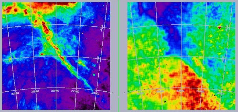
Figure 2: Right Panel: Map of the DIRBE-corrected IRAS 100 $\mu$m data for a portion of the sky centered on $l\sim 280^{\rm{o}}$, $b\sim-45^{\rm{o}}$. The “shadowing” filament discussed in this paper runs diagonally across the image. Left Panel: Map of the ROSAT $\frac{1}{4}$ keV data for the same projection. Regions of missing data are black. By comparing these two maps, we can see that the “shadowing” filament corresponds with the sharply delineated arch of low $\frac{1}{4}$ keV surface brightness in the soft X-ray map where the filament blocks soft X-ray emission from the Galactic halo. The finite “zero-point” surface brightness ($\sim 400\times 10^{-6}$ counts s^-1 arcmin^-2) is due to the Local Bubble emission. Both panels are adaptations of figures in Snowden et al. (1997).

The intensity of resonance line photons from O VI along extended lines of sight through the Local Bubble, the Galactic halo, and intervening regions is reported elsewhere (Shelton et al., 2001; Dixon, et al., 2001; Shelton, 2002; Welsh et al, 2002). Here, we wish to measure only the O VI intensity of the Local Bubble, and so must block the photons from external regions. To do so, we employ the “shadowing” strategy oft-used in X-ray analyses. In the ideal shadowing observation, an opaque object blocks the emission originating beyond it, so that the observed emission originates between the viewer and the object. For the shadowing object, we have chosen a filament in the Southern Galactic hemisphere (see Figure 2). Penprase et al. (1998) estimated the distance to the filament as 230$\pm$30 pc, which places the filament between the Local Bubble and the Galactic halo. Penprase et al. (1998) also estimated the mean color excess ($E(B-V)$) of the filament as 0.17$\pm$0.05 magnitudes, implying an absorbing column density of $N_{H}=8.4\pm 2.5\times 10^{20}$ cm^-2. This is consistent with the column density implied by the Schlegel, Finkbeiner, & Davis (1998) IRAS 100 $\mu$m measurement of $\sim 7.3$ MJy sr^-1, which when scaled by the 100 $\mu$m to $N_{H}$ converstion relation for the southern hemisphere listed in Snowden et al. (2000), yields a column density of $9.9\times 10^{20}$ cm^-2. For this color excess and the extinction curve and parameterization presented in Fitzpatrick (1999), $89^{+5}_{-11}\%$ of the O VI photons originating beyond the filament should be blocked.

As a demonstration of the filament’s “shadowing” function, we note it’s ability to block soft X-rays. (The theoretical extinction of $\sim\frac{1}{4}$ X-rays is larger than that of ultraviolet photons.) The ROSAT $\frac{1}{4}$ keV band image (see Figure 2) reveals an obvious soft X-ray depression coincident with the filament. The surface brightness seen in the direction of the filament and attributed to the Local Bubble is $590\times 10^{-6}$ counts s^-1 arcmin^-2, while the “off-filament” surface brightness is $\sim 1300\times 10^{-6}$ counts s^-1 arcmin^-2 (K. D. Kuntz, private communication). Not surprisingly, the filament has already been used successfully in ROSAT soft X-ray shadowing analyses (Wang & Yu, 1995; Snowden et al., 2000).

One potential difficulty in using this region of the sky is posed by Penprase et al. (1998)’s suggestion that the filament may be part of a supernova remnant. If this were the case, then the foreground O VI intensity should be attributed to both the Local Bubble and the supposed supernova remnant. Because the results or our study are upper limits, this point is unimportant. Observations of the targeted region, the bulbous portion of the filament around $l=278.6^{\rm{o}},b=-45.3^{\rm{o}}$, are discussed in the following section.

3 Observations and Data Reduction

The FUSE focal plane assembly contains four spectrograph entrance apertures. The largest, the low resolution (LWRS) aperture measuring 30” $\times$ 30”, is used for observations of diffuse sources. Furthermore, the FUSE instrument includes multiple approximately co-aligned channels. Four of the channels (LiF 1A, SiC 1A, LiF 2B, and SiC 2B) cover the 1032, 1038 Å region. Of these, the LiF 1A is most sensitive and least prone to scattered light problems in the 1032, 1038 Å region. We use this channel for our O VI analysis. In addition, we use the LiF 1A, SiC 1B, LiF 2A, and SiC 2A channels for the C I, C II, C III, N I, N II, N III, Mg II, Si II, S II, S III, S IV, S VI, Fe II, and Fe III analyses.

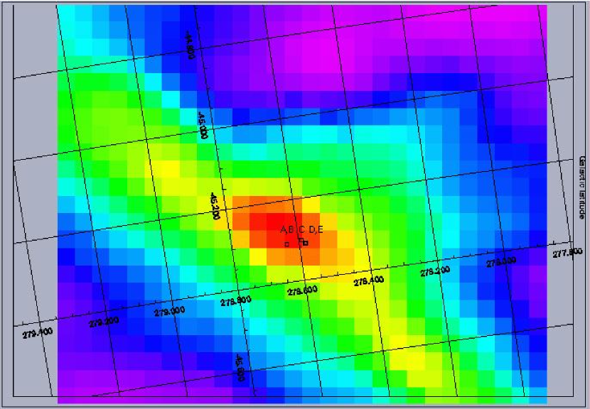
Figure 3: Infrared 100$\mu$m image of an opaque and bulbous section of the filament. The overlayed boxes indicate the placement of the FUSE LWRS aperture. The B1290101 and B1290102 observations point in the same direction but with slightly different angles. Their aperture location is labeled “A” and “B” on this image. At their location, the 100$\mu$m intensity is 7.2 MJy sr^-1. The I2050601 pointing direction is labeled “C”. For this observation, the location of the FUSE aperture crosses a pixel boundary in the 100$\mu$m map, such that the average 100$\mu$m intensity is 7.2 MJy sr^-1. The I2050510 and I2050501 pointing directions are also nearly identical. They are labeled “D” and “E” on the map and have 100$\mu$m values of 7.0 MJy sr^-1. The lowest 100$\mu$m intensity on this image is 2.0 MJy sr^-1. Note that the filament’s infrared brightness in excess of the background level implies a degree of obscuration that is in very good agreement with Penprase et al. (1998)’s quoted E(B-V).

The raw data consists of multiple observations of three nearly coincident directions (see Table 1 and Figure 3). The combined exposure time (after subtracting time when the spacecraft was exposed to the Earth’s South Atlantic Anomaly, time when the detectors recorded anomalous bursts, etc.) for the LiF 1A observations is 228 ksec. The other detectors have had differing useful exposure times. Most notably, detector 2 malfunctioned during the I2050501 observation, reducing the total observation time with the LiF 2A and SiC 2A channels. The observations can be grouped according to pointing direction. Henceforth, the combined I2050501 and I1050510 observations of $l=278.58^{\rm{o}},b=-45.31^{\rm{o}}$ will be denoted by “I20505”, the I2050601 observation of $l=278.59^{\rm{o}},b=-45.30^{\rm{o}}$ will be denoted by “I20506”, and the combined B1290101 and B1290102 observations of $l=278.63^{\rm{o}},b=-45.31^{\rm{o}}$ will be denoted by “B12901”. Each of these three datasets was processed using version 2.1 of the CALFUSE pipeline (Sahnow et al., 2000; Dixon, Kruk & Murphy, 2002). We set the appropriate pipeline switches, so as to 1.) exclude counts that produced pulseheights outside the expected range for cosmic photons (the chosen CALFUSE pipeline cutoffs were 4 and 12 in the standard arbitrary units for the older datasets (I20505 and I20506) and 4 to 31 for the newer dataset (B12901)) in order to reduce the detector background noise, and 2.) disallow automatic background subtraction, enabling us to more accurately calculate the signal to noise of the results.

Figure 4 displays the 1020 to 1045 Å region of the LiF 1A spectra for the three pointing directions. At this stage, the absolute wavelength scales are still inaccurate, though the relative wavelength scales of the pipeline spectra are accurate to several detector pixels (about 0.035 Å in the LiF 1A spectrum). The largest sources of systematic error in the following intensity calculations are the uncertainties in the solid angle of the aperture and effective area calibration. Both the LWRS’s solid angle (30 arcsec $\times$ 30 arcsec) and the LiF 1A effective area calibration are thought to be accurately known to $\sim 10\%$. Thus, the systematic uncertainty in intensity measurements will be $\sim 14\%$.

4 Spectral Analysis

In order to determine the absolute wavelength scales for the LiF 1A spectra from the three pointings, we used the airglow emission lines as reference wavelengths. We then co-added the spectra from the three pointings and shifted to the Local Standard of Rest (LSR) reference frame. The 1020 to 1045 Å region of the resulting satellite-night and day $+$ night spectra are displayed in Figure 5.

We found the continuum level in the satellite-night spectrum by fitting a smooth curve to the surrounding spectral region. We then searched the residual spectrum for emission features. None were found in close proximity to the O VI resonance line rest wavelengths in the LSR reference frame. If cosmic features had existed, their widths would have equaled or exceeded the instrumental width function, their signals would have been calculated from the numbers of counts in excess of the continuum within the extraction width, and their random uncertainties would have been calculated from the square roots of the numbers of spectral counts (not residual counts) within the extraction width. We have followed this method, using the total instrumental width (generously set to 0.43 Å) as the extraction width, to determine the upper limits. The “signal” and 1 sigma statistical uncertainty intensities for the O VI resonance lines at their rest wavelengths in the LSR reference frame are 180 $\pm$ 330 and -180 $\pm$ 310 photons cm^-2 s^-1 sr^-1, for the 1032 and 1038 Å lines, respectively. These measurements are subject to the above mentioned systematic uncertainties of $14\%$. We validated our technique by applying the following alternate extraction technique to sample spectra. We fit the spectrum to a continuum and small emission feature, then varied the size of the feature to determine the 1 sigma uncertainties. The results were similar to those found by applying our techniques to the same spectra.

When the satellite-day portions of the data sets were added, the spectrum became more ragged. From the variations between the I20505, I20506, and B12901 satellite-day spectra we surmise that the raggedness is primarily due to scattered light. For the combined day and night spectrum, the “signal” and 1 sigma statistical uncertainty intensities are 20 $\pm$ 230 and 80 $\pm$ 210 photons cm^-2 s^-1 sr^-1, for the 1032 and 1038 Å lines, respectively. The measurements are subject to the $14\%$ systematic uncertainties. For reference, Table 2 tabulates these results and lists the tightest 1 and 2 sigma upper limits. The 1 and 2 sigma upper limits were calculated from the unrounded numbers.

We also searched for C I, C II, C III, N I, N II, N III, Mg II, Si II, S II, S III, S IV, S VI, Fe II, and Fe III emission lines in the spectra taken with the LiF 1A, SiC 1B, LiF 2A, and SiC 2A detector segments. We relied on the satellite-night portion of the data when we searched for emission lines which also appear strongly in the solar spectrum (i.e. C III, Curdt et al. (1997)), appear weakly in the terrestrial airglow spectrum (i.e. N II, Feldman et al. (2001)), or are significantly stronger in the satellite-day portion of the data than in the satellite-night portion of the data (i.e. C II). The only signals detected were marginally significant intensities of C III and N II (see Table 3).

5 Discussion

These observations are the first to place tight upper limits on the intensity of the O VI emission from the Local Bubble (2 sigma upper limits on the 1032 and 1038 Å emission lines of 530 and 500 photons cm^-2 s^-1 sr^-1, respectively). The theoretical ratio of the intensity of 1032 to 1038 Å photons is 2.0 to 1.0. Using the 2.0 to 1.0 ratio and the 1032 Å line upper limit yields a 2 sigma doublet upper limit of 800 photons cm^-2 s^-1 sr^-1 or $1.5\times 10^{-8}$ ergs cm^-2 s^-1 sr^-1.

5.1 Comparisons with Local Bubble Models

Breakout Model: $4\times 10^{4}$ K, Overionized Bubble

In this scenario, a series of supernova explosions and winds has created a hot, youthful bubble. It is assumed that the bubble expanded rapidly as it broke into a low density region. The rapid, adiabatic expansion cooled the bubble faster than the ions could recombine, so that the gas now has a temperture of 4 to $6\times 10^{4}$ K, but still highly ionized and X-ray emissive (Breitschwerdt & Schmutzler, 1994; Breitschwerdt, 2001). Because the transition zones between the bubble plasma and the embedded cool clouds will be cooler than the collisional ionizational equilibrium temperature for O VI, they need not be rich in O VI ions.

In the Breitschwerdt (2001) model, the Local Bubble has a radius of 115 pc, density (of electrons, Breitschwerdt, personal communication) of $2.4\times 10^{-2}$ cm^-3, and pressure (presumably thermal) of $\sim 2000$ K cm^-3. Thus, the plasma temperature is approximately $4.3\times 10^{4}$ K. Lacking published estimates for the O VI intensity, we will calculate it from the above values and the emission equation in Shull & Slavin (1994). The intensity calculation also requires the ratio of electrons to hydrogen nuclei in a solar abundance plasma (1.2), the solar abundance of oxygen ($8.5\times 10^{-4}$, Grevesse & Anders (1989)), and an estimate of the fraction of oxygen atoms in the O VI ionization level. During the plasma’s extraordinary cooling history, it has experienced some degree of recombination, as evidenced by the strong lines of C III, O III, and O IV in Breitschwerdt (2001)’s predictions. Here, we take the lower limit on recombinations of oxygen to the O VI state as that of a $5\times 10^{5}$ K collisional ionizational equilibrium plasma. In this case, the fraction of oxygen in the O VI state is 0.037 (Mazzotta et al., 1998; Schmutzler & Tscharnuter, 1993). As the plasma recombines further, the O VI/oxygen fraction increases, and, due to recombinations of O VII, does not decrease until the most of the oxygen has recombined to O I and O II. An upper limit on the extent of the recombinations is taken from the isochoric cooling predictions of Schmutzler & Tscharnuter (1993) at the model temperature, again yielding an O VI to oxygen fraction of 0.037. We take 0.037 as our estimate, noting that the O VI/oxygen ratio and the intensity prediction may be higher. The resulting intensity estimate, $\sim 1900$ photons cm^-2 s^-1 sr^-1, is more than twice the 2 sigma upper limit established in this paper.

For this calculation, the O VI ions are assumed to be mixed throughout the remnant. If the assumed abundance of metal atoms were reduced from the solar value, then the soft X-ray scaling relationships used in finding the model parameters would need to be adjusted to a similar degree. As a result, the model parameters would need to be adjusted, probably leading to a bigger, denser, and/or hotter bubble. As far as the predicted O VI intensity is concerned, these adjustments would probably offset the hypothetical abundance adjustment.

Not only is there a significant discrepancy between our null result and the intensity calculated from the model, there is a factor of 20 difference between the observed O VI column density ($\sim 1.6\times 10^{13}$ cm^-2, Shelton & Cox (1994), Oegerle et al. (2002), see below) and the column density calculated from the model ($2.7\times 10^{14}$ cm^-2), and a significant discrepancy between the 2 sigma upper limit on the observed C III 977 Å intensity ($7300$ photons cm^-2 s^-1 sr^-1) and the published C III prediction ($\geq 8500$ photons cm^-2 s^-1 sr^-1, Figure 2 Breitschwerdt (2001)). The number and magnitude of these discrepancies practically eliminate this class of models.

Generalized Multi-Phase Model of the Local Bubble

The lesson learned from evaluating the previous model was that a bubble consisting of a single, moderate temperature, overionized plasma is disallowed because it contains too many O VI ions and emits too many photons from its O VI and C III ions. Furthermore, a bubble consisting of a single, collisional ionizational equilibrium plasma which is hot enough to produce the observed soft X-ray surface brightness is disallowed because it contains too few O VI ions (see below). In contrast, suppose the Local Bubble contains multiple distinct plasmas, a collisional ionizational equilibrium, million degree, X-ray emissive plasma and a several hundred thousand degree, O VI-rich plasma. Cool clouds are also known to lie within the Local Bubble so such a topology is reasonable. One example of an allowed form is a hot bubble, bounded by transition temperature gas and possibly containing additional transition zones around embedded cool clouds. Here, we consider such a generalized multi-phase model, in order to determine if it can meet the observational constraints or if more unusual circumstances are required.

The hotter component in this multi-phase model accounts for the observed soft X-rays, but few O VI photons. Based on the temperature found from a soft X-ray analysis ($10^{6.1}$ K, assuming collisional ionizational equilibrium, Kuntz & Snowden (2000)), the observed ROSAT  R12 band countrate seen toward this part of the filament (590 $\times 10^{-6}$ counts s^-1 arcmin^-2, K. D. Kuntz, private communication), the conversion between the ROSAT  R12 band countrate and the emission measure ($1\times 10^{-6}$ counts s^-1 arcmin^-2 $=$ $7.15\times 10^{-6}$ cm^-6 pc^-1, Snowden et al. (1997)), the fraction of oxygen atoms in the O VI ionization level at this temperature ($3.2\times 10^{-3}$, Mazzotta et al. (1998)), the solar abundance of oxygen ($8.5\times 10^{-4}$, Grevesse & Anders (1989)), the ratio of free electrons to hydrogen nuclei (1.2), and the electron-impact excitation rate coefficient of Shull & Slavin (1994), we estimate that the $\sim 10^{6}$ K region produces only $\sim$60 photons cm^-2 s^-1 sr^-1 in the O VI resonance line doublet from a column density of only $5\times 10^{11}$ O VI ions cm^-2.

The primary source of O VI ions and resonance line photons would be the transition temperature gas. Althought it need not be in collisional ionizational equilibrium, we will assume its temperature is between $1\times 10^{5}$ K and $1\times 10^{6}$ K for the following calculations. The Local Bubble’s column density of O VI ions is roughly $1.6\times 10^{13}$ cm^-2 (see following subsection). By assuming that the gas is in thermal pressure balance with the soft X-ray emitting plasma ($P_{th}/k\sim$ 15,000 K cm^-3, Snowden et al. (1998)), we estimate its electron density. The temperature is not well known, but most of the O VI ions are likely to be near their ionizational equilibrium temperature ($3.2\times 10^{5}$ K), and the emission equation is relatively insensitive to temperature for $1\times 10^{5}\stackrel{{\scriptstyle<}}{{\sim}}T\stackrel{{\scriptstyle<}}{{\sim}}1\times 10^{6}$ K. An O VI-rich plasma, with the above column density, a temperature of $6.3\times 10^{5}$ K, and a thermal pressure of 15,000 K cm^-3 emits 450 photons cm^-2 s^-1 sr^-1, which is within the observational 2 sigma upper limit on the intensity. Similar plasmas with temperatures as low as $\sim 1\times 10^{5}$ K emit even less intense O VI radiation. Thus, a two phase model could meet the observational constraints without requiring unobserved astrophysics or unusual conditions.

Simulations of A Hot Bubble with Transition Zones

In this section, we examine the multi-phase bubble simulations of Smith & Cox (2001) and the evaporating cloud simulations of Slavin (1989). In the models of Smith & Cox (2001), the Local Bubble resulted from two or three supernova explosions occurring up to several million years ago. The interior of the structure consists of hot ($\sim 10^{6}$ K), nearly collisional ionizational equilibrium plasma, while the periphery of the structure consists of an intermediate temperature transition zone. Although the simulations do not explicitly include the transition zones surrounding the embedded cool clouds, such zones are thought to harbor O VI ions (Slavin, 1989; Oegerle et al., 2002) and so should contribute to the flux of O VI resonance line photons. Here, we will use the simulations of Slavin (1989), which predict their intensity.

After performing several hydrodynamical simulations, Smith & Cox (2001) decided that the best model lies intermediate between their various simulations. Their simulations yield predicted O VI intensities ranging from 190 to more than 9,500 photons cm^-2 s^-1 sr^-1, (after the extra factor of $4\pi$ in their Figure 19 (Smith, private communication) is divided out). To this intensity must be added the intensity emitted by the transition zone on the local cloud and, possibly, transition zones on other cool clouds embedded in the Local Bubble. For the transition zone on the cool cloud surrounding the Sun, Slavin (1989) predicted an O VI doublet intensity of 250 photons cm^-2 s^-1 sr^-1. The sum of the Smith & Cox (2001) and Slavin (1989) predictions (440 to $\geq 9800$ photons cm^-2 s^-1 sr^-1) marginally overlaps the 2 sigma upper limit reported in this paper. If other cool clouds reside along the line of sight, then the predicted O VI intensity would be even higher. Thus, this particular model is heavily constrained by the null results. We would have lost confidence in this type of model had it not been possible to simultaneously satisfy the O VI emission, O VI column density, and ROSAT soft X-ray constraints with the above generalized multiphase model.

5.2 Limits on Electron Density, Pressure, Pathlength, Cooling Timescale

Here, we will combine the intensity upper limit with column density estimates taken from the literature in order to calculate the upper limits on the electron density and thermal pressure in the O VI-rich plasma. The first data-derived estimate of the typical O VI column density of the Local Bubble ($N_{OVI}\sim 1.6\times 10^{13}$ cm^-2, (Shelton & Cox, 1994)) was found via a statistical analysis of several dozen Copernicus lines of sight, most of which terminated far beyond the Local Bubble. Later, FUSE observed a couple dozen lines of sight entirely within the Local Bubble. The work of Welsh et al (2002) and Oegerle et al. (2002) suggest that the O VI column density within the Local Bubble may be as little as a few $\times 10^{12}$ cm^-2 in some directions, but that the column density increases roughly with distance from the Sun and the total column density along a 100 pc radial path is consistent with values of $7\times 10^{12}$ cm^-2 to $1.6\times 10^{13}$ cm^-2. Here, we take the column density from the published survey (i.e. $1.6\times 10^{13}$ cm^-2).

Using the emission equation of Shull & Slavin (1994), the above column density, the 2 sigma upper limit on the doublet intensity, and the temperature at which O VI is most prevalent in collisional ionizational equilibrium plasmas ($T=3.2\times 10^{5}$ K, Mazzotta et al. (1998)) yields an estimated upper limit for the electron density, $n_{e}$, of 0.021 cm^-3. Thus, the estimated upper limit for the thermal pressure, from $P_{th}/k=1.92n_{e}T$, is $13,000$ K cm^-3. If the temperature were significantly higher than the assumed temperature, then the pressure would be greater. If it is not, then the total (thermal and nonthermal) pressure in the O VI-rich region of the Local Bubble (presumably the transition zones) could be brought into balance with that of the X-ray emitting region of the Local Bubble (presumably the interior, $P_{th}/k\sim$ 15,000 K cm^-3) by assuming that the cooler, denser O VI-rich regions have a greater non-thermal pressure than the hotter, more rarefied X-ray emitting region.

Furthermore, the O VI-rich material occupies a pathlength ($\Delta l$) of at least ${\sim}5900N_{OVI}/n_{e}$ in cm, (incorrectly type-set in Shelton (2002)), or $\stackrel{{\scriptstyle>}}{{\sim}}0.15$ pc, consistent with transition zones. The cooling timescale solely due to cooling through the O VI doublet is

$$t=\frac{\frac{3}{2}kT}{4\pi{\rm{(sr)}}I_{OVI}}N_{OVI}\frac{n_{T}}{n_{ovi}},$$ (1)

where $k$ is Boltzman’s constant, $n_{ovi}$, $n_{oxy}$, ${n_{H}}$, and ${n_{T}}$ are the densities of O VI ions, oxygen atoms, hydrogen nuclei, and particles, respectively, sr means steradians, and $n_{ovi}/n_{oxy}=0.24$ at $3.2\times 10^{5}$ K (Mazzotta et al., 1998). Thus, the cooling timescale due solely to O VI resonance line emission is at least $2.0\times 10^{6}$ years. These Local Bubble values are tabulated in Table 4, along with the Galactic halo values calculated in the following subsection.

5.3 Galactic Halo

Previous FUSE studies of emission from O VI in the interstellar medium (ISM) outside of superbubbles or supernova remnants observed far longer paths (Shelton et al. (2001); Dixon, et al. (2001); Shelton (2002); and Welsh et al (2002)). In each of those cases, the instrument had been directed toward a high Galactic latitude direction ($|b|>40^{\rm{o}}$). Given that the local region contributes little O VI resonance line intensity, the vast majority of the intensity observed on the relatively unobscured, high latitude observations must originate beyond the Local Bubble. Extragalactic sources are ruled out by the velocities of the observed emission features and so this emission presumably resides in the Galactic thick disk and halo. Subtracting the Local Bubble’s doublet intensity from the averages of the intensities observed by Shelton et al. (2001); Dixon, et al. (2001); Shelton (2002); and Welsh et al (2002) leaves 3500 to 4300 photons cm^-2 s^-1 sr^-1, attributable to the Galactic halo.

The column density through the halo is roughly $3.0\times 10^{14}$ cm^-2 (Savage et al., 2000). Thus, using the method of Section 5.2, we find the electron density in the halo’s O VI-rich gas to be 0.0050 to 0.0061 cm^-3. The thermal pressure is 3100 to 3800 K cm^-3, consistent with the range of total pressures in models of the Galactic thick disk and lower halo (Boulares & Cox, 1990; Ferrière, 1995). The pathlength is at least 110 pc. The cooling timescale is 7 to $8\times 10^{6}$ years.

6 Summary

• The Local Bubble’s O VI intensity has been examined through a shadowing observation directed toward $l=278.6^{\rm{o}},b=-45.3^{\rm{o}}$. No emission was seen. The tightest 2 sigma upper limits on the 1032 and 1038 Å emission lines are 530 and 500 photons cm^-2 s^-1 sr^-1, respectively. Given the theoretical intensity ratio (2.0 to 1.0), the tightest 2 sigma upper limit on the resonance line doublet is 800 photons cm^-2 s^-1 sr^-1.

• The class of models in which the Local Bubble is assumed to be a single, moderate temperature ($\sim 4\times 10^{4}$ K), extremely overionized plasma is virtually ruled out. The 2 sigma upper limits on the O VI and C III intensities exceed the model predictions, as does the observed O VI column density. The class of models in which the Local Bubble is a single, hot ($10^{6}$ K), collisional ionizational equilibrium plasma are also ruled out. Such a model could not produce the observed O VI column density. However, the combined O VI and ROSAT soft X-ray observations allow models in which the Local Bubble contains multiple, separate phases. The X-ray emission can be attributed to the hot zone and the O VI ions can be attributed to transition zones. Existing simulations of a multiphase bubble combined with simulations of a single evaporating cloud are tightly constrained by our 2 $\sigma$ upper limit on the doublet intensity. Considering that multiple clouds are expected to reside along the typical line of sight, the expected O VI intensity falls well below the upper limit, suggesting that transition zones differ from current models.

• The estimated 2 sigma upper limit on the electron density in the Local Bubble’s O VI-bearing plasma is 0.021 cm^-3. If the temperature is near the collisional ionizational equilibrium temperature for O VI ($3.2\times 10^{5}$ K), then the thermal pressure is $\leq 13,000$ K cm^-3, which is weaker than that of the soft X-ray emissive portion of the Local Bubble. The discrepancy could be resolved if the O VI-bearing gas were to have a greater than assumed temperature or a significant nonthermal pressure.

• The timescale for cooling soley due to the O VI resonance line emission is proportional to the thermal energy in the gas and inversely proportional to the O VI intensity. For the Local Bubble, this timescale is $\geq 2\times 10^{6}$ years.

• The Galactic halo’s O VI doublet intensity has been found by subtracting the Local Bubble result from other observations. It is 3500 to 4300 photons cm^-2 s^-1 sr^-1.

• The Galactic halo’s intensity implies an electron density of $\sim 0.0050$ to $\sim 0.0061$ cm^-3. If the temperature is near the collisional ionizational equilibrium temperature for O VI  then the thermal pressure is $\sim 3100$ to $\sim 3800$ K cm^-3. This pressure is consistent with the total pressure estimates in models of the thick disk and lower halo.

• The O VI in the Galactic halo cools on a timescale ($t\propto$ thermal energy / O VI intensity) of 7 to $8\times 10^{6}$ years.

Table 1:

Program Id	Start Date	LiF 1A Exposure Time	Night Time	LWRS Direction
Number	(UT)	(ksec)	(ksec)	(l,b)
I2050501	Aug. 21, 1999	84.5	27.8	$278.58^{\rm{o}},-45.31^{\rm{o}}$
I2050510	Aug. 24, 1999	17.7	4.5	”
I2050601	Aug. 27, 1999	18.2	5.6	$278.59^{\rm{o}},-45.30^{\rm{o}}$
B1290101	Aug. 13, 2001	52.5	9.6	$278.63^{\rm{o}},-45.31^{\rm{o}}$
B1290102	Aug. 16, 2001	55.0	15.4	”
Total		227.7	62.8	$278.6^{\rm{o}},-45.3^{\rm{o}}$

Table 2: Upper Limits on the O VI Emission Lines

Emission Region	Intensity (ph s-1 cm-2 sr-1)	Intensity (ph s-1 cm-2 sr-1)
	Night Only	Day$+$Night
	Combined Dataset
1031.93 Å	$180\pm 330\pm 14\%$	$20\pm 230\pm 14\%$
1037.62 Å	$-180\pm 310\pm 14\%$	$80\pm 210\pm 14\%$
	Tightest 1 Sigma Limits, incl. $14\%$ Systematic Uncertainty
1031.93 Å		280
1037.62 Å	150
	Tightest 2 sigma Limits, incl. $14\%$ Systematic Uncertainty
1031.93 Å		530
1037.62 Å	500

Table 3: Other Transitions

Species	Rest Wavelength	Intensity	Notes
	(Å)	(photons cm-2 s-1 sr-1)
C I	945.6 Å	$-300\pm 390$	B
C I	1122.3 Å	$-240\pm 370$	N
C II	1037.0 Å	$30\pm 290$	N
C III	977.0 Å	$4700\pm 1300$	N, SiC 1B
”	”	$2600\pm 1000$	N, SiC 2A
N I	954.0 Å	$-200\pm 740$	N
N II	916.7 Å	$2300\pm 1100$	N, SiC 1B
N III	991.6 Å	$-170\pm 850$	N
Mg II	946.7 Å	$-430\pm 680$	N
Si II	1023.7 Å	$-200\pm 190$	B
S II	906.9 Å	$-240\pm 1100$	N
S III	1015.5 Å	$170\pm 240$	B
S IV	1062.7 Å	$-390\pm 300$	N
S IV	1073.0 Å	$300\pm 280$	N
S VI	933.4 Å	$170\pm 690$	N
S VI	944.5 Å	$1000\pm 840$	N
Fe II	1144.9 Å	$270\pm 220$	B
Fe III	1122.5 Å	$-700\pm 350$	N

The reported error bars reflect the 1 sigma random uncertainties. All measurements are subject to the net systematic uncertainty of $14\%$. “B” denotes both the day and night portions of the data and “N” denotes the satellite-night portion of the data. In cases where airglow emission or scattered light affected the satellite-day data for the spectral region of interest or the satellite-day spectrum undulated substantially, we used only the satellite-night portion of the data. We also used the night spectrum for the Mg II observation because it led to a more constraining upper limit. For the measurements in this table, the tighter pulseheight cuts were used in processing the B12901 portion of the data.

Table 4:

Region	$n_{e}$	$P_{th}/k$	$\Delta l$	$t$
	(cm-3)	(K cm-3)	(pc)	(yr)
Local Bubble	$\leq 0.021$	$\leq 1.3\times 10^{4}$	$\stackrel{{\scriptstyle>}}{{\sim}}0.15$	$\geq 2\times 10^{6}$
Galactic Halo	0.0050 to 0.0061	3100 to 3800	$\stackrel{{\scriptstyle>}}{{\sim}}110$	7 to $8\times 10^{6}$

Figure 4: The 1020 to 1045 Å region of the LiF 1A spectra extracted from the B12901 (top panel), I20505 (middle panel) and I20506 (bottom panel) data. Each panel presents the spectra drawn from the satellite-night portion of the data (raised by $6\times 10^{4}$ photons s^-1 cm^-2 sr^-1 Å^-1), the spectrum drawn from the satellite-day portion of the data (raised by $3\times 10^{4}$ photons s^-1 cm^-2 sr^-1 Å^-1), and the spectrum drawn from the combined day and night data (unadjusted). The wavelength scales have not yet been corrected. Each spectrum has been binned by 11 pixels The Earth’s atmospheric airglow lines are marked with $\oplus$ symbols. The wavelengths of the O VI resonance lines and C II 3s² S_1/2 to 2p² P_3/2 line are marked on the top and middle panels. No O VI or C II emission is evident.

Figure 5: Co-added spectrum from the night-only portion of the data (top panel) and co-added spectrum from both day and night portions of the data (bottom panel). The wavelength scale has been corrected and shifted to the LSR reference frame. The spectral data has been binned by 11 pixels. The night spectrum is flat, except for variations due to noise. No excess intensity around 1032, 1038, or 1037 Å is observed. Neither is there a 1032 Å feature in the “Day$+$Night” spectrum. The sharp thin emission feature near 1031.5 Å is only present during the satellite-day portion of the data and so is not attributable to interstellar material. Similar features have appeared in previous daytime blank sky observations (Shelton et al., 2001). The “Day$+$Night” spectrum wavers significantly between 1036 and 1038 Å, preventing us from searching for the 1037 and 1038 Å lines.

References

- Bochkarev (1987) Bochkarev, N. G. 1987, Ap & SS, 138, 229
- Boulares & Cox (1990) Boulares, A., & Cox, D. P. 1990, ApJ, 365, 544
- Bloch et al. (1986) Bloch, J. J., Jahoda, K., Juda, M., McCammon, D., Sanders, W. T., Snowden, S. L 1986, ApJ, 308, 59
- Breitschwerdt (2001) Breitschwerdt, D. 2001, Astrophysics and Space Sciece, 276, 163
- Breitschwerdt & Schmutzler (1994) Breitschwerdt, D., & Schmutzler, T. 1994, Nature, 371, 774
- Curdt et al. (1997) Curdt, W., Feldman, U., Laming, J. M., Wilhelm, K., Schühle, U., & Lemair, P. 1997, A & AS, 126, 281
- Dixon, Kruk & Murphy (2002) Dixon, W. V., Kruk, J. W., & Murphy, E. M. 2002, CALFUSE Pipeline Reference Guide, http:fuse.pha.jhu.eduanalysispipelinereference.html
- Dixon, et al. (2001) Dixon, W. V., Sallmen, S., Hurwitz, M., & Lieu, R. 2001, ApJ, 552, L69
- Egger (1993) Egger, R. J. 1993, PhD Thesis, Technische Universität, München
- Egger & Aschenbach (1995) Egger, R. J., & Aschenbach, B. 1995, A & A, 294, 25
- Feldman et al. (2001) Feldman, P. D., Sahnow, D. J., Kruk, J. W., Murphy, E. M., Moos, H. W. 2001, JGR, 106, 8119
- Ferrière (1995) Ferrière, K. 1995, ApJ, 441, 281
- Fitzpatrick (1999) Fitzpatrick, E. L. 1999, PASP, 111, 63
- Frisch (1986) Frisch, P. 1986, AdSpR, 6, 345
- Frisch (1981) Frisch, P. 1981, Nature, 293, 377
- Grevesse & Anders (1989) Grevesse, N., & Anders, E. 1989, in AIP Conf. Proc. 183, Cosmic Abundances, p. 1
- Gry et al. (1995) Gry, C., Lemonon, L., Vidal-Madjar, A., Lemoine, M., & Ferlet, R. 1995, A & A, 302, 497 xs
- Hutchinson et al. (1998) Hutchinson, I. B., Warwick, R. S., & Willingale, R. 1998, Lecture Notes in Physics, vol.506, The Local Bubble and Beyond, ed. D. Breitschwerdt, M. J. Freyberg, & J. Truemper, pp. 283-286
- Juda et al. (1991) Juda, M., Bloch, J. J., Edwards, B. C., McCammon, D., Sanders, W. T., Snowden, S. L., Zhang, J. 1991, ApJ, 367, 182
- Knapp (1975) Knapp, G. R. 1975, AJ, 80, 111
- Kuntz & Snowden (2000) Kuntz, K. D., & Snowden, S. L. 2000, ApJ, 543, 195
- Lallement & Bertin (1992) Lallement, R., & Bertin, P. 1992, A & A, 266, 479
- Lallement et al. (1995) Lallement, R., Ferlet, R. Lagrange, A. M., Lemoine, M. & Vidal-Madjar, A. 1995, A & A, 304, 461
- Mazzotta et al. (1998) Mazzotta, P., Mazzitelli, G., Colafrancesco, S., & Vittorio, N. 1998, A & AS, 133, 403
- McCammon et al. (1983) McCammon, D., Burrows, D. N., Sanders, W. T., & Kraushaar, W. L. 1983, ApJ, 269, 107
- Oegerle et al. (2002) Oegerle, W. R., Jenkins, E. B., Shelton, R. L., Bowen, D. V. & Chayer, P., 2002, in preparation
- Penprase et al. (1998) Penprase, B. E., Lauer, J., Aufrecht, J., & Welsh, B. Y. 1998, ApJ, 492, 617
- Sahnow et al. (2000) Sahnow, D. J., et al. 2000, ApJ, 538, L7
- Sanders et al. (2001) Sanders, W. T., Edgar, Richard J., Kraushaar, W. L., McCammon, D., Morgenthaler, J. P. 2001, ApJ, 554, 694
- Savage et al. (2000) Savage, B. D., et al. 2000, ApJ, 538, L27
- Schlegel, Finkbeiner, & Davis (1998) Schlegel, D. J., Finkbeiner, D. P., & Davis, M. 1998, ApJ, 500, 525
- Schmutzler & Tscharnuter (1993) Schmutzler, T., & Tscharnuter, W. M. 1993, A & A, 273, 318
- Sfeir et al. (1999) Sfeir, D. M., Lallement, R., Crifo, F., & Welsh, B. Y. 1999, A & A, 346, 785
- Shelton (2002) Shelton, R. L. 2002, ApJ, 569, 758
-
Shelton & Cox (1994)
Shelton, R. L., & Cox, D. P. 1994, ApJ, 434, 599
- Shelton et al. (2001) Shelton, R. L., et al. 2001, ApJ, 560, 730
- Shull & Slavin (1994) Shull, J. M., & Slavin, J. D. 1994, ApJ, 427, 784
- Slavin (1989) Slavin, J. D. 1989, ApJ, 346, 718
- Smith & Cox (2001) Smith, R. K., & Cox, D. P. ApJS, 2001, 134, 283
- Snowden et al. (1997) Snowden, S. L., Egger, R., Freyberg, M. J., McCammon, D., Plucinsky, P. P., Sanders, W. T., Schmitt, J. H. M. M., Truemper, J., & Voges, W. 1997, ApJ, 485, 125
- Snowden et al. (1998) Snowden, S. L., Egger, R., Finkbeiner, D. P., Freyberg, M. J., Plucinsky, P. P. 1998, ApJ, 493, 715
- Snowden et al. (2000) Snowden, S. L., Freyberg, M. J., Kuntz, K. D., & Sanders, W. T. 2000, ApJS, 128, 171
- Wang & Yu (1995) Wang, Q. D., & Yu, K. C. 1995, AJ, 109, 698
- Welsh et al (2002) Welsh, B. Y., Sallmen, S., Sfeir, D., Shelton, R. L., & Lallement, R. 2002, A & A, 394, 691