Diffusion in supersonic, turbulent, compressible flows

Abstract

We investigate diffusion in supersonic, turbulent, compressible flows. Supersonic turbulence can be characterized as network of interacting shocks. We consider flows with different rms Mach numbers and where energy necessary to maintain dynamical equilibrium is inserted at different spatial scales. We find that turbulent transport exhibits super-diffusive behavior due to induced bulk motions. In a comoving reference frame, however, diffusion behaves normal and can be described by mixing length theory extended into the supersonic regime. (Accepted for publication in Phys. Rev. E)

I Introduction

Laboratory and terrestrial gases and liquids are usually well described by incompressible flows (e.g. Lesieur ). In contrast, the dynamical behavior of typical astrophysical gases, are characterized by poorly understood highly compressible supersonic turbulent motion (see e.g. VS00 ). For example, the large observed linewidths in large molecular clouds show direct evidence for the presence of chaotically oriented velocity fields with magnitudes in excess of the sound speed. This random motion carries enough kinetic energy to counterbalance and sometimes overcompensate the effects of self-gravity of these clouds WBM00 . The intricate interplay between supersonic turbulence and self-gravity determines the overall dynamical evolution of these clouds and their observable features such as their density structure, the star formation rate within them, and their lifetimes. Thus, it is importance for the description of many astrophysical systems to understand in detail the momentum and heat transfer properties of compressible turbulent gases.

Some important clues on the nature and efficiency of mixing associated with the clouds’ supersonic turbulence can be constrained by the observed metallicity distribution of the stars formed within them. In the Pleiades cluster, stars which emerged from the same molecular cloud have nearly identical metal abundance W02 . This astronomical context therefore imposes a strong motivation for a general analysis of the transport and mixing processes in compressible supersonically turbulent media.

Analytical and numerical studies of diffusion processes are typically restricted to certain families of statistical processes, like random walk MK00 or remapping models or certain Hamiltonian systems I92 . The direct numerical modeling of turbulent physical flows mostly concentrates on incompressible media (e.g. DS97 ; MKM99 ; OL01 ), but some studies have been extended into the weakly compressible regime CKM95 ; HCB95 ; PPW92 ; PPW94 ; PPSW99 . Although highly compressible supersonic turbulent flows have been studied in several specific astrophysical contexts PW00 ; SPWHW00 ; SOG98 ; OGS99 ; OSG01 ; M99 ; KHM00 ; SMH00 ; HMK01 ; HZMLN01 ; BM02 ; PVP95 ; PV98 ; VPP95 ; VS92 ; BVS99 ; BP99 ; BCP01 ; PN99 ; PZN00 ; BNP02 ; GPPL01 , the diffusion properties of such flows have not been investigated in detail.

It is the goal of this paper to analyze transport phenomena in supersonic compressible turbulent flows and to demonstrate that – analogous to the incompressible case – a simple mixing length description can be found even for strongly supersonic and highly compressible turbulence. We first briefly recapitulate in Section II the Taylor formalism for describing the efficiency of turbulent diffusion in subsonic flows. In Section III we describe the numerical method which we use to integrate the Navier-Stokes equation. In Section IV we report the diffusion coefficient obtained in our numerical models, and in Section V we introduce an extension of the well known mixing length approach to diffusion into the supersonic compressible regime. Finally, in Section VI we summarize our results.

II A statistical description of turbulent diffusion

Transport properties in fluids and gases can be characterized by studying the time evolution of the second central moment of some representative fluid-elements’ displacement in the medium,

$$\xi^{2}_{\vec{r}}(t-t^{\prime})=\langle[\vec{r}_{i}(t)-\vec{r}_{i}(t^{\prime})]^{2}\rangle_{i}\;,$$ (1)

where the average $\langle\cdot\rangle_{i}$ is taken over an ensemble of passively advected tracer particles $i$ (e.g. dye in a fluid, or smoke in air) that are placed in the medium at a time $t^{\prime}$ at positions $\vec{r}_{i}(t^{\prime})$; or where the average is taken over the fluid molecules themselves (or equivalently, over sufficiently small and distinguishable fluid elements). The dispersion in one spatial direction, say along the $x$-coordinate, is $\xi^{2}_{x}(t-t^{\prime})=\langle[x_{i}(t)-x_{i}(t^{\prime})]^{2}\rangle_{i}$. For isotropic turbulence it follows that $\xi^{2}_{x}=\xi^{2}_{y}=\xi^{2}_{z}=1/3\;\xi^{2}_{\vec{r}}$. For fully-developed stationary turbulence, the initial time $t^{\prime}$ can be chosen at random and for simplicity is set to zero in what follows.

The quantity $\xi_{\vec{r}}(t)$ can be associated with the diffusion coefficient $D$ as derived for the classical diffusion equation,

$$\frac{\partial n}{\partial t}=D\vec{\nabla}^{2}n\;,$$ (2)

where $n(\vec{r}_{i},t)$ is the probability distribution function (pdf) for finding a particle $i$ at position $\vec{r}_{i}(t)$ at time $t$ when it initially was at a location $\vec{r}_{i}(0)$. This holds if the particle position is a random variable with a Gaussian distribution B49 . In the classical sense, $n(\vec{r},t)$ may correspond to the contaminant density in the medium. Equation 2 holds for normal diffusion processes and for time scales larger than the typical particles’ correlation time scale $\tau$.

In general, however, the Lagrangian diffusion coefficient is time dependent and can be defined as

$$D(t)=\frac{d\xi^{2}_{\vec{r}}(t)}{dt}=2\langle\vec{r}_{i}(t)\cdot\vec{v}_{i}(t)\rangle_{i}\;,$$ (3)

where $\vec{v}_{i}(t)=d\vec{r}_{i}(t)/dt$ is the Lagrangian velocity of the particle. The diffusion coefficient along one spatial direction, say along the $x$-coordinate, follows accordingly as $D_{x}=d\xi^{2}_{x}(t)/dt=2\langle x_{i}(t)v_{x.i}(t)\rangle_{i}$. Equation 3 holds for homogeneous turbulence with zero mean velocity. From $\vec{r}_{i}(t)=\vec{r}_{i}(0)+\int_{0}^{t}\vec{v}_{i}(t^{\prime})dt^{\prime}$ it follows that

$$D(t)=2\left\langle\left[\vec{r}_{i}(0)+\int_{0}^{t}\vec{v}_{i}(t^{\prime})dt^{\prime}\right]\cdot\vec{v}_{i}(t)\right\rangle_{i}=2\int_{0}^{t}\langle\vec{v}_{i}(t^{\prime})\cdot\vec{v}_{i}(t)\rangle_{i}dt^{\prime}\;.$$ (4)

The above expression allows us to related $D(t)$ to the trace of the Lagrangian velocity autocorrelation tensor ${\rm{tr}}\,{\cal C}(t-t^{\prime})=\langle\vec{v}_{i}(t^{\prime})\cdot\vec{v}_{i}(t)\rangle_{i}$ as

$$D(t)=2\int_{0}^{t}{\rm{tr}}\,{\cal C}(t-t^{\prime})dt^{\prime}=2\int_{0}^{t}{\rm{tr}}\,{\cal C}(t^{\prime})dt^{\prime}\;,$$ (5)

a result which was derived by Taylor already 1921 T21 . This formulation has the advantage that it is fully general and that it allows us to study anomalous diffusion processes. Note, that strictly speaking any transport process with $\xi_{\vec{r}}(t)$ not growing linearly in time is called anomalous diffusion. This is always the case for time intervals shorter than the correlation time $\tau$, but sometimes anomalous diffusion can also occur for $t\gg\tau$. If $\xi_{\vec{r}}(t)\propto t^{\alpha}$ and if $\alpha<1$ transport processes are called subdiffusive, if $\alpha>1$ they are called superdiffusive Lesieur ; I92 ; CMMV99 ; LM00 . Studying transport processes directly in terms of the particle displacement, i.e. Equation 1, is useful when attempting to find simple approximations to the diffusion coefficient $D(t)$ for example in a mixing length approach.

III Numerical Method

In order to utilize the above formalism, we carry out a series of numerical simulation of supersonic turbulent flows. A variety of numerical schemes can be used to describe the time evolution of gases and fluids. By far the most widely-used and thoroughly-studied class of methods is based on the finite difference representations of the equations of hydrodynamics (e.g. P77 ). In the most simple implementation, the fluid properties are calculated on equidistant spatially fixed grid points in a Cartesian coordinate system. Finite difference schemes have well defined mathematical convergence properties, and can be generalized to very complex, time varying, non-equidistant meshes with arbitrary geometrical properties. However, it is very difficult to obtain a Lagrangian description, which is essential when dealing with compressible supersonic turbulence with a high degree of vorticity. Methods that do not rely on any kind of mesh representation at all are therefore highly desirable.

For the current investigation we use smoothed particle hydrodynamics (SPH), which is a fully Lagrangian, particle-based method to solve the equations of hydrodynamics. The fluid is represented by an ensemble of particles, where flow properties and thermodynamic observables are obtained as local averages from a kernel smoothing procedure (typically based on cubic spline functions) B90 ; M92 . Each particle $i$ is characterized by mass $m_{i}$, velocity $\vec{v}_{i}$ and position $\vec{r}_{i}$ and carries in addition density $\rho_{i}$, internal energy $\epsilon_{i}$ or temperature $T_{i}$, and pressure $p_{i}$. The SPH method is commonly used in the astrophysics community because it can resolve large density contrasts simply by increasing the particle concentration in regions where it is needed. This versatility is important for handling compressible turbulent flows where density fluctuations will occur at random places and random times. The same scheme that allows for high spatial resolution in high-density regions, however, delivers only limited spatial resolution in low-density regions. There, the number density of SPH particles is small and thus the volume necessary to obtain a meaningful local average tends to be large. Furthermore, SPH requires the introduction of a von Neumann Richtmyer artificial viscosity to prevent interparticle penetration, shock fronts are thus smeared out over two to three local smoothing lengths. Altogether, the performance and convergence properties of the method are well understood and tested against analytic models and other numerical schemes, for example in the context of turbulent supersonic astrophysical flows PRL ; KB00 ; KB01 ; KHM00 , and its intrinsic diffusivity is sufficiently low to allow for the current investigation of turbulent diffusion phenomena L99 .

To simplify the analysis we assume the medium is infinite and isotropic on large scales, and consider a cubic volume which is subject to periodic boundary conditions. The medium is described as an ideal gas with an isothermal equation of state, i.e. pressure $p$ relates to the density $\rho$ as $p=c^{2}_{\rm s}\rho$ with $c_{\rm s}$ being the speed of sound. Throughout this paper we adopt normalized units, where all physical constants (like the gas constant), total mass $M$, mean density $\langle\rho\rangle$, and the linear size $L$ of the cube all are set to unity. The speed of sound is $c_{\rm s}=0.05$, hence, the sound crossing time through the cube follows as $t_{\rm sound}=20$. In all models discussed here, the fluid is represented by an ensemble of $205\,379$ SPH particles which gives sufficient resolution for the purpose of the current analysis.

Supersonic turbulence is known to decay rapidly PRL ; SOG98 ; PN99 ; BM99 ; MB00 ; BM00 . Stationary turbulence in the interstellar medium therefore requires a continuous energy input. To generate and maintain the turbulent flow we introduce random Gaussian forcing fields in a narrow range of wavenumbers such that the total kinetic energy contained in the system remains approximately constant. We generate the forcing field for each direction separately and simply add up the three contributions. Thus, we excite both, solenoidal as well as compressible modes at the same time. The typical ratio between the solenoidal and compressible energy component is between 2:1 and 3:1 in the resulting turbulent flow (see e.g. Figure 8 in KHM00 .). We keep the forcing field fixed in space, but adjust its amplitude in order to maintain a constant energy input rate into the system compensating for the energy loss due to dissipation (for further details on the method see M99 ; KHM00 ). This non-local driving scheme allows us to exactly control the (spatial) scale which carries the peak of the turbulent kinetic energy. It is this property that motivated our choice of random Gaussien fields as driving source. In reality the forcing of turbulence in the interstellar medium is likely to be a multi-scale phenomenon with appreciable contributions from differential rotation (i.e. shear) in the Galctic disk and energy input from supernovae explosions ending the lives of massive stars MK03 . Comparable to the values observed in interstellar gas, we study flows with Mach numbers in the range 0.5 to 10, where we define the Mach number from the one-dimensional rms velocity dispersion $\sigma_{v}$ as ${\cal M}=\sigma_{v}/c_{\rm s}$. For each value of the Mach number we consider three different cases, one case where turbulence is driven on large scales only (i.e. with wavenumbers $k$ in the interval $1\leq k\leq 2$), intermediate-wavelength turbulence ($3\leq k\leq 4$), and small-scale turbulence ($7\leq k\leq 8$), as summarized in Table 1. Note that our models are not subject to global shear because of the adopted periodic boundary conditions. We call turbulence ”large scale” when the Fourier decomposition of the velocity field is dominated by the largest scales possible for the considered volume $L^{3}$, i.e. the system becomes isotropic and homogeneous only on scales larger than $L$. On scales below $L$ it may exhibit a considerable degree of anisotropy. This is most noticeable in the case $1\leq k\leq 2$, because wavenumber space is very poorly sampled and variance effects become significant. The system is dominated by one or two large shock fronts that cross through the medium. In the interval $7\leq k\leq 8$ the number of Fourier modes contribution to the velocity field is large, and the system appears more isotropic and homogeneous already on distances smaller than $L$. This trend is clearly visible in Figure 1.

Table 1: Model properties

(1)	(2)	(3)	(4)	(5)	(6)	(7)	(8)	(9)	(10)	(11)	(12)	(13)
model	$k$	${\cal M}$	$t_{\rm cross}$	$\bar{\sigma}_{x}$	$\bar{\sigma}_{y}$	$\bar{\sigma}_{z}$	$D_{x}(\infty)$	$D_{y}(\infty)$	$D_{z}(\infty)$	$2\bar{\sigma}_{x}/k$	$2\bar{\sigma}_{y}/k$	$2\bar{\sigma}_{z}/k$
0$\ell$	$1..2$	0.6	35.3	0.030	0.028	0.027	0.027	0.021	0.019	0.030 – 0.060	0.028 – 0.057	0.027 – 0.054
0i	$3..4$	0.5	39.1	0.026	0.026	0.025	0.010	0.010	0.009	0.013 – 0.017	0.013 – 0.017	0.013 – 0.017
0s	$7..8$	0.4	46.2	0.021	0.022	0.022	0.005	0.005	0.005	0.005 – 0.006	0.005 – 0.006	0.005 – 0.006
1$\ell$	$1..2$	1.9	10.4	0.106	0.084	0.098	0.140	0.069	0.111	0.106 – 0.213	0.084 – 0.167	0.098 – 0.196
1i	$3..4$	1.9	10.6	0.097	0.096	0.092	0.042	0.047	0.038	0.048 – 0.065	0.048 – 0.064	0.046 – 0.061
1s	$7..8$	1.7	11.5	0.086	0.089	0.087	0.025	0.026	0.024	0.021 – 0.024	0.022 – 0.025	0.022 – 0.025
2$\ell$	$1..2$	3.1	6.5	0.173	0.129	0.158	0.223	0.103	0.169	0.173 – 0.346	0.129 – 0.257	0.158 – 0.315
2i	$3..4$	3.1	6.4	0.167	0.155	0.151	0.084	0.071	0.063	0.083 – 0.111	0.077 – 0.103	0.075 – 0.100
2s	$7..8$	3.2	6.3	0.154	0.163	0.157	0.044	0.054	0.047	0.038 – 0.044	0.041 – 0.046	0.039 – 0.045
3$\ell$	$1..2$	5.2	3.8	0.301	0.252	0.227	0.314	0.245	0.169	0.301 – 0.603	0.252 – 0.505	0.227 – 0.454
3i	$3..4$	5.8	3.5	0.261	0.287	0.316	0.131	0.189	0.233	0.130 – 0.174	0.143 – 0.191	0.158 – 0.211
3s	$7..8$	5.8	3.4	0.297	0.288	0.289	0.106	0.092	0.091	0.074 – 0.085	0.072 – 0.082	0.072 – 0.083
4$\ell$	$1..2$	8.2	2.4	0.467	0.318	0.444	0.693	0.241	0.558	0.467 – 0.933	0.318 – 0.635	0.444 – 0.887
4i	$3..4$	9.7	2.1	0.451	0.478	0.520	0.248	0.323	0.349	0.225 – 0.301	0.239 – 0.319	0.260 – 0.347
4s	$7..8$	10.4	1.9	0.532	0.513	0.519	0.194	0.167	0.170	0.133 – 0.152	0.128 – 0.147	0.130 – 0.148

1. column: Model identifier, with the letters $\ell$, $i$, and $s$ standing for large-scale, intermediate-wavelength, and short-wavelength turbulence, respectively.
2. column: Driving wavelength intervall.
3. column: Mean Mach number, defined as ratio between the time-averaged one-dimensional velocity dispersion $\bar{\sigma}_{v}=3^{-1/2}(\bar{\sigma}^{\,2}_{x}+\bar{\sigma}^{\,2}_{y}+\bar{\sigma}^{\,2}_{y})^{1/2}$ and the isothermal sound speed $c_{\rm s}$, ${\cal M}=\bar{\sigma}_{v}/c_{\rm s}$. The values for the different velocity components $x$, $y$, and $z$ may differ considerably, especially for large-wavelength turbulence. Please recall from Section III that the speed of sound is $c_{\rm s}=0.05$, and thus the sound crossing time $t_{\rm sound}=20$.
4. column: Average shock crossing time through the computational volume.
5. to 7. column: Time averaged velocity dispersion along the three principal axes $x$, $y$, and $z$, e.g. for the $x$-component $\bar{\sigma}_{x}^{\,2}=\int_{0}^{t}\langle(v_{x.i}(t^{\prime})-\langle v_{x.i}(t^{\prime})\rangle_{i})^{2}\rangle_{i}dt^{\prime}/t$.
8. to 10. column: Mean-motion corrected diffusion coefficients along the three principal axes computed from Equation 3 for time intervals $t\gg\tau$.
11. to 13. column: Predicted values of the mean motion corrected diffusion coefficients $D^{\prime}_{x}$, $D^{\prime}_{y}$, and $D^{\prime}_{z}$ from extending mixing length theory into the supersonic regime (Section V).

Similar to any other numerical calculations, the models discussed here fall short of describing real gases in comprehensive details as they cannot include all physical processes that may act on the medium. In interstellar gas clouds, transport properties and chemical mixing will not only be determined by the compressible turbulence alone, but the density and velocity structure is also influenced by magnetic fields, chemical reactions, and radiation transfer processes. Furthermore, all numerical models are resolution limited. The turbulent inertial range in our large-scale turbulence simulations spans over about 1.5 decades in wavenumber. This range is considerably less than what is observed in interstellar gas clouds. The same limitation holds for the Reynolds numbers achieved in the models, they fall short of the values in real gas clouds by several orders of magnitude. Nevertheless, despite these obvious shortcomings, the results derived here do characterize global transport properties in interstellar gas clouds and in other supersonically turbulent compressible flows.

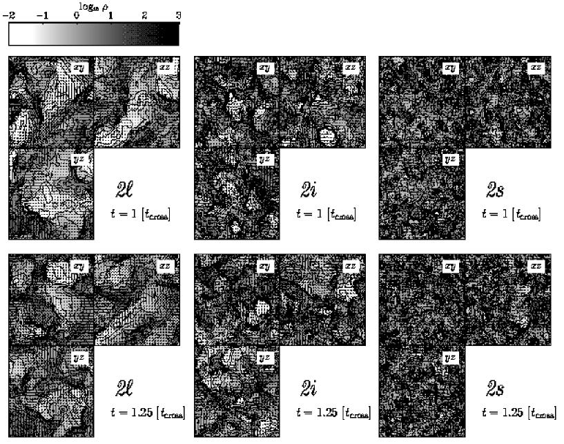
Figure 1: Density and velocity structure of models 2$\ell$, 2i, and 2s (from left to right). The panels show cuts through the center of the computational volume normal to the three principal axes of the system, after one shock crossing time $t_{\rm cross}=L/\sigma_{v}\approx 6.5$ and 1/4 $t_{\rm cross}$ later. Density is scaled logarithmically as indicated in the greyscale key at the upper left side. The maximum density is $\sim 100$, while the mean density is one in the normalized units used. Vectors indicate the velocity field in the plane. The rms Mach number is ${\cal M}\approx 3.1$. Large-scale turbulence (2$\ell$) is dominated by large coherent density and velocity gradients leading a large degree of anisotropy, whereas small-scale turbulence (2s) exhibits noticeable structure only on small scales with the overall density structure being relatively homogeneous and isotropic.

Figure 2: Time evolution of the mean flow velocity $\langle\vec{v}_{i}(t)\rangle_{i}$ in models 2$\ell$, 2i, and 2s. Time $t$ and velocity $v$ are given in normalized units (Section III).

IV Transport properties

Supersonic turbulence in compressible media establishes a complex network of interacting shocks. Converging shock fronts locally generate large density enhancements, diverging flows create rarefied voids of low gas density. The fluctuations in turbulent velocity fields are highly transient, as the random flow that creates local density enhancements can disperse them again. The life time of individual shock-generated clumps corresponds to the time interval for two successive shocks to pass through the same location in space, which in turn depends on the length scale of turbulence and on the Mach number of the flow.

The velocity field of turbulence that is driven at large wavelengths is found to be dominated by large-scale shocks which are very efficient in sweeping up material, thus creating massive coherent density structures. The shock passing time is rather long, and shock-generated clumps can travel quite some distance before begin disrupted. On the contrary, when energy is inserted mainly on small scales, the network of interacting shocks is very tightly knit. Clumps have low masses and the time interval between two shock fronts passing through the same location is small, hence, swept-up gas cannot travel far before being dispersed again.

The density and velocity structure of three models with large-, intermediate-, and small-wavelength turbulence is visualized in Figure 1. It shows cuts through the centers of the simulated volume. As turbulence is stationary, all times are equivalent, and the snapshot in the upper panel is taken at some arbitrary time. The lower panel depicts the system some time interval later corresponding to $1/4$ shock crossing time through the cube. One clearly notices markable differences in the density and velocity field between the three models.

IV.1 Transport properties in an absolute reference frame

In order to drive supersonic turbulence and to maintain a given rms Mach number in the flow, we use a random Gaussian velocity field with zero mean to ‘agitate’ the fluid elements at each timestep. However, despite the fact that the driving scheme has zero mean, the system is likely to experience a net acceleration and develop an appreciable drift velocity, because of the compressibility of the medium. This evolutionary trend is well illustrated in Figure 2 which plots the time evolution of the three components of the mean velocity for models 2$\ell$, 2i, and 2s, with rms Mach numbers ${\cal M}\approx 3.1$, where turbulence is driven on (a) large (i.e. with small wavenumbers $1\leq k\leq 2$), (b) intermediate ($3\leq k\leq 4$), and (c) small scales (with $7\leq k\leq 8$). The net acceleration is most pronounced when turbulent energy is inserted on the global scales, as in this case larger and more coherent velocity gradients can build up across the volume compared to small-scale turbulence.

The tendency for the zero-mean Gaussian driving mechanisms to induce significant center-of-mass drift velocities in highly compressible media can be understood as follows. Suppose the gas is perturbed by one single mode in form of a sine wave. If the medium is homogeneous and incompressible, equal amounts of mass would be accelerated in the forward as well as in the backward direction. But, if the medium is inhomogeneous, there would be an imbalance between the two directions and the result would be a net acceleration of the system. If the density distribution remains fixed, this acceleration would be compensated by an equal amount of deceleration after half a period, and the center of mass would simply oscillate. However, if the system is highly compressible and the driving field is a superposition of plane waves, the density distribution would change continuously (and randomly). Any net acceleration at one instance in time would not be completely compensated after some finite time interval later. This will only occur for $t\rightarrow\infty$ assuming ergodicity of the flow. Subsequently, the system is explected to develop a net flow velocity in some random direction for $t<\infty$. This effect is most clearly noticeable for long-wavelength turbulence, where density and velocity structure is dominated by the coherent large-scale structure. But the effect is small for turbulence that is excited on small scales, because in this limit, there is a large number of accelerated ‘cells’ which in turn compensate for another’s acceleration.

Figure 3: Time evolution of the diffusion coefficient $D(t)=d\langle[\vec{r}_{i}(t)-\vec{r}_{i}(0)]^{2}\rangle_{i}/dt$ for models 2$\ell$, 2i, and 2s computed in an absolute reference frame. All units are normalized as described in Section III.

The property that the compressible turbulent flows are likely to pick up average drift velocities, even when driven by Gaussian fields with zero mean, has implications for the transport coefficients. Figure 3 shows the time evolution of the absolute (Eulerian) diffusion coefficients $D_{x}$, $D_{y}$, and $D_{z}$ in each spatial direction computed from Equation 1. Note that for stationary turbulence, only time differences are relevant and one is free to chose the initial time. In order to improve the statistical significance of the analysis, we obtain $D(t)$ and $\xi_{\vec{r}}(t)$ by further averaging over all time intervals $t$ that ‘fit into’ the full timespan of the simulation.

Due to the (continuous) net acceleration experienced by the system, the quantity $\xi_{\vec{r}}^{2}(t)$ grows faster than linearly with time, even for intervals much larger than the correlation time $\tau$, i.e. for $\tau\ll t<\infty$. The system resides in a superdiffusive regime, where $D(t)$ does not saturate. Instead, $D(t)$ grows continuously with time, which is most evident in model 2$\ell$ of large-scale turbulence. The ever increasing drift velocity $\langle\vec{v}_{i}(t)\rangle_{i}$ causes strong velocity correlations leading continuous growth of the velocity autocorrelation tensor $\int_{0}^{t}{\rm tr}\,{\cal C}(t^{\prime})dt^{\prime}$. This net motion, however, can be corrected for, allowing us to study the dispersion of particles in a reference frame that moves along with the average flow velocity of the system.

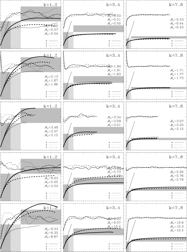
Figure 4: Time evolution of the diffusion coefficient $D^{\prime}(t)=d\xi^{2}_{i}/dt$ computed in a reference frame that follows the average flow velocity (thick line, axis scaling on the left ordinate), i.e. is centered on $\langle\vec{r}_{i}(t)\rangle_{i}=\int_{0}^{t}\langle\vec{v}_{i}(t^{\prime})\rangle_{i}dt^{\prime}$. Velocity dispersions along the three major axes $x$, $y$, and $z$ are each normalized to unity using the time-averaged one-dimensional Mach number $\cal M$ (as indicated in each plot) together with the given value of the sound speed $c_{\rm s}$ (thin lines, axis scaling on the right ordinate). Times are rescaled to the rms shock crossing time through the simulated cube $t_{\rm cross}=L/\sigma_{v}=L/({\cal M}c_{\rm s})$. Details for each model are given in Table 1. The horizontal gray shaded area indicates the mixing length prediction for $t\rightarrow\infty$, and the vertical gray and light gray shaded areas show a time interval of $\tau=L/(k{\cal M}c_{\rm s})$ and $2\tau$, respectively. For $t\ll\tau$ diffusion should be anomalous and coherent, with $D^{\prime}(t)$ growing linearly with time. The expected behavior from mixing length theory in this regime is indicated by the straight line originating at $t=0$. It indeed gives a good fit. Note that all models driven on large scales ($1\leq k\leq 2$) exhibit a considerable degree of anisotropy, manifested by different rms Mach numbers $\cal M$ along the three principal axes and different values $D^{\prime}(t)$. For the models with intermediate-scale and small-scale driving anisotropy effects are increasingly less important.

IV.2 Transport properties in flow coordinates

In order to gain further insight into the transport properties of compressible supersonic turbulent flows, we study the time evolution of the relative (Lagrangian) diffusion coefficient. In this prescription,

$$D^{\prime}(t)=\frac{d\xi^{2}_{\vec{r}}(t)}{dt}$$

is obtained relative to a frame of reference which comoves with the mean motion of the system $\langle\vec{v}_{i}(t)\rangle_{i}$ on the trajectory $\langle\vec{r}_{i}(t)\rangle_{i}=\int_{0}^{t}\langle\vec{v}_{i}(t^{\prime})\rangle_{i}dt^{\prime}$. Then, $\xi^{2}_{\vec{r}}(t-t^{\prime})=\langle[(\vec{r}_{i}(t)-\langle\vec{r}_{i}(t)\rangle_{i})-(\vec{r}_{i}(t^{\prime})-\langle\vec{r}_{i}(t^{\prime})\rangle_{i})]^{2}\rangle_{i}$ (see Equation 1).

In Figure 4, we show the evolution of $D^{\prime}(t)$ for each coordinate direction for the complete suite of models. The rms Mach numbers range from about 0.5 to 10, each considered for three cases where turbulence is driven on large, intermediate, and small scales, respectively. The plots are rescaled such that the time-averaged one-dimensional rms velocity dispersion $\bar{\sigma}_{v}$ is normalized to unity (for each direction separately). We also rescale the time $t$ with respect to the average shock crossing time scale through the computational volume, $t_{\rm cross}=L/\bar{\sigma}_{v}$. Recall that $L=1$, and note that $\bar{\sigma}_{v}$ usually differs between the three spatial directions because of the variance effects, especially in models of large-scale turbulence.

In Figure 4, we demonstrate that the magnitude of $D^{\prime}(t)$ saturates for large time intervals $t>\tau$ in all directions. In a reference frame that follows the mean motion of the flow, diffusion in compressible supersonically turbulent media indeed behaves in a normal manner. For small time intervals $t<\tau$, however, the system still exhibits an anomalous diffusion even with the mean-motion correction. In this regime $D^{\prime}(t)$ grows roughly linearly with time. For $t>\tau$ the diffusion coefficient $D^{\prime}(t)$ reaches an asymptotic limit. This result holds for the entire range of Mach numbers studied and for turbulence that is maintained by energy input on very different spatial scales.

From Figure 4, we find that diffusion in compressible supersonic turbulent flows follows a universal law. It can be obtained by using the rms Mach number (together with the sound speed $c_{\rm s}$) as characterizing parameter for rescaling the velocity dispersion $\sigma_{v}$, and the rms shock crossing time scale through the volume $t_{\rm cross}=L/({\cal M}c_{\rm s})$ for rescaling the time. The normalized diffusion coefficient $D^{\prime}(t)$ exhibits a universal slope of two at times $t<\tau$ (i.e. in the superdiffusive regime), and approaches a constant value that depends only on the length scale but not on the strength (i.e. the resulting Mach number) of the mechanism that drives the turbulence. Even for highly compressible supersonic turbulent flows it is possible to find simple scaling relations to characterize the transport properties — analogous to the mixing length description of diffusive processes in incompressible subsonic turbulent flows.

V A mixing length description

Incompressible turbulence is often described in terms of a hierarchy of turbulent eddies, where each eddy contains multiple eddies of smaller size on the lower levels of the hierarchy, while itself being part of turbulent eddy at larger scales R22 ; K41 ; O41 . At each level of the hierarchy, an eddy is characterized by a typical lengthscale $\tilde{\ell}$ and a typical velocity $\tilde{v}$. The typical lifetime of an eddy is its ‘turn-over’ time $\tau=\tilde{\ell}/\tilde{v}$. This mixing length prescription is an attempt to characterize the flow properties in terms of the typical scales $\tilde{\ell}$ and $\tilde{v}$. For example, this classical picture defines an effective ‘eddy’ viscosity $\mu=\rho\tilde{\ell}\tilde{v}$, where $\rho$ is the density. The mixing length $\tilde{\ell}$ is interpreted to be the turbulent analogue of the mean free path of molecules in the kinetic theory of gases, with $\tilde{v}$ being the characteristic velocity of the turbulent fluctuation.

In such a model, the velocities of gas molecules within an eddy are strongly correlated within a time interval $t<\tau$. They all follow the eddy rotation; the diffusion process is coherent. However, for $t\gg\tau$ the velocities of gas molecules become uncorrelated, as the eddy has long been destroyed and dispersed. Hence, the velocity autocorrelation function vanishes for large time intervals, ${\cal C}(t)\rightarrow 0$ for $t\rightarrow\infty$. Diffusion becomes incoherent as in Brownian motion or the random walk. The diffusion coefficient in the mixing length approach simply is $D(t)\approx 2\tilde{v}^{2}t$ in the regime $t<\tau$, which follows from replacing $\vec{r}(t)$ by $\tilde{v}t$ and $\vec{v}(t)$ by $\tilde{v}$ in Equation 3. As the largest correlation length is the eddy size, $\vec{r}(t)$ is substituted by $\tilde{\ell}=\tilde{v}\tau$ for times $t\gg\tau$, and the classical mixing length theory yields $D(t)\approx 2\tilde{\ell}\tilde{v}=2\tilde{v}^{2}\tau={\rm constant}$.

Compressible, supersonic, turbulent flows rapidly build up a network of interacting shocks with highly transient density and velocity structure. Density fluctuations are generated by locally converging flows, and their lifetimes are determined by the time $\tau$ between two successive shock passages. This time interval is determined by the typical shock velocity, which is roughly the rms velocity of the flow, i.e. the Mach number times the sound speed, $\sigma_{v}={\cal M}c_{\rm s}$. It also depends on the length scale at which energy is inserted into the system to maintain the turbulence, which in our case is $L/k$ with $k$ being the driving wavenumber and $L$ being the size of the considered region (recall that in our models $L$ is unity). This length scale is also the typical traveling distance before two shocks interact with each other. As basic ingredients for a supersonic compressible mixing length description we can thus identify:

$${\rm shock~{}travel~{}length:} \tilde{\ell}\approx L/k,$$ (6)

$${\rm rms~{}velocity:} \tilde{v}\approx\sigma_{v}={\cal M}c_{\rm s}.$$ (7)

The Lagrangian velocity correlation time scale, $\tau$, is analogeous to the time interval during which shock-generated density fluctuation remains unperturbed and moves coherently before it is being dispersed by the interaction with a new shock front. This time interval is equivalent to the time scale a shock travels along its ‘mean free path’ $\tilde{\ell}$ with an rms velocity $\tilde{v}$. This crossing time is $\tau=\tilde{\ell}\tilde{v}\approx\sigma_{v}\,L/k$. For $t<\tau$ gas molecules can travel coherently within individual shock generated density fluctuations, and the diffusion coefficient in the mixing length prescription follows as

$$D^{\prime}(t)\approx 2\tilde{v}^{2}t\approx 2\sigma_{v}^{2}t\;.$$ (8)

$D^{\prime}(t)$ grows linearly with time with slope $2\sigma_{v}^{2}$. For large times, $t\gg\tau$, $D^{\prime}(t)$ approaches a constant value,

$$D^{\prime}(t)\approx 2\tilde{v}^{2}\tau\approx 2\sigma_{v}\,L/k\;.$$ (9)

This mixing length approach (Equations 8 and 9) suggests a unique scaling dependence of the diffusion coefficients in supersonic compressible flows on the Mach number $\cal M$ and on the length scale $\tilde{\ell}$ of the most energy containing modes with respect to the total size $L$ of the system considered.

We can use $\cal M$ (together with the given value of the sound speed) to normalize the rms velocity: $\sigma_{v}={\cal M}c_{\rm s}\mapsto\sigma_{v}^{\prime}=1$. And we can also rescale the time with respect to the rms shock crossing time scale through the total volume, which is $t_{\rm cross}=L/\sigma_{v}=L/({\cal M}c_{\rm s})=t_{\rm sound}/{\cal M}$ with $t_{\rm sound}=L/c_{\rm s}$ being the sound crossing time, so that $t\mapsto t^{\prime}=t/t_{\rm cross}$. From this normalization procedure, we get $D^{\prime}(t)\mapsto D^{\prime\prime}(t^{\prime})=D^{\prime}(t)\,{\cal M}c_{\rm s}L$ and obtain the following universal profile for the diffusion coefficient,

$$D^{\prime\prime}(t^{\prime})=2t^{\prime} {\rm~{}for~{}}\; t^{\prime}\ll 1/k{\rm~{}~{}~{}~{}and}$$ (10)

$$D^{\prime\prime}(t^{\prime})=2/k {\rm~{}for~{}}\; t^{\prime}\gg 1/k\;.$$ (11)

Note that this result holds for each velocity component separately, as the results in Figure 4 indicate. In this case $\sigma_{v}$ stands for $\sigma_{x}$, $\sigma_{y}$, or $\sigma_{z}$ in Equations 8 and 9, and it hold for the total diffusion coefficient, when using $\sigma_{v}=({\sigma_{x}^{2}+\sigma_{y}^{2}+\sigma_{z}^{2}})^{1/2}$ instead.

Figure 5: Comparison between mixing length predictions and numerical models. At the left we plot he normalized, mean-motion corrected diffusion coefficient $D^{\prime\prime}(t^{\prime})$ for $t\rightarrow\infty$, and at the right its slope $dD^{\prime\prime}(t^{\prime})/dt^{\prime}$ for $t^{\prime}\ll 1/k$. For each suite of models, large-scale, intermediate-scale, and small-scale turbulence, respectively (as indicated by the forcing wavenumber $k$ at the top of each plot), we separately show the three velocity components (as indicated at the bottom). The different Mach numbers in each model suite are denoted by different symbols (as identified at the right-hand side of each plot). The dotted lines give the corresponding prediction of the mixing-length theory, $D^{\prime\prime}(t^{\prime})=2/k$ and $dD^{\prime\prime}(t^{\prime})/dt^{\prime}=2$, respectively, where we take $k$ to be the maximum wavenumber of the forcing scheme (indicated at the top of each plot).

The validity of the mixing length approximation is quantified in Figure 5 which plots the mixing length predictions against the values obtained from the numerical models. For large-scale and intermediate scale turbulence, the mixing length approach gives very satisfying results, only for small-scale turbulence it underestimates the diffusion strength. This disparity probably has to do with the numerical resolution of the code, in the sense that driving wavenumbers of $k\approx 8$ come close to the dissipation scale of the method and hence the inertial range of turbulence is limited KHM00 . That limitation leads to an effective driving for the turbulent motion on somewhat larger scales than $1/8$. Consequently, it leads to a stronger diffusion, i.e. somewhat larger diffusion coefficients than those predicted by Equations 10 and 11. The same numerical effects also account for the slightly shallower slope of $D^{\prime}(t)$ for $t\ll\tau$ for models $7\leq k\leq 8$.

Figures 4 and 5 indicate that the classical mixing length theory can be extended from incompressible (subsonic) turbulence into the regime of supersonic turbulence of highly compressible media. In this case, driving length $\tilde{\ell}$ and rms velocity dispersion $\sigma_{v}={\cal M}c_{\rm s}$ act as characteristic length and velocity scales in the mixing length approach. Note, that this only applies to mean-motion corrected transport. In general (i.e. in an absolute reference frame), supersonic turbulence in compressible media leads to superdiffusion as visualized in Figure 3.

VI Summary

We studied diffusion processes in supersonically turbulent, compressible media. To drive turbulence and maintain the desired rms Mach number in the flow, we insert energy into the system at a pre-specified rate and over a given spatial scale using random Gaussian fields. In our numerical models, the adopted magnitude of the rms Mach numbers range from ${\cal M}=0.5$ to ${\cal M}=10$, and turbulence was driven on large, intermediate, and small scales, respectively.

Supersonic turbulence in compressible media establishes a complex network of interacting shocks. Converging shock fronts locally generate large density enhancements, diverging flows create voids of low gas density. The fluctuations in turbulent velocity fields are highly transient, as the random flow that creates local density enhancements can disperse them again.

Due to compressibility, supersonically turbulent flows will usually develop noticeable drift velocities, especially when turbulence is driven on large scales, even when it is excited with Gaussian fields with zero mean. This tendency has consequences for the transport properties in an absolute reference frame. The flow exhibits super-diffusive behavior (see also B01 ). However, when the diffusion process is analyzed in a comoving coordinate system, i.e. when the induced bulk motion is being corrected, the system exhibits normal behavior. The diffusion coefficient $D(t)$ saturates for large time intervals, $t\rightarrow\infty$.

By extending classical mixing length theory into the supersonic regime we propose a simple description for the diffusion coefficient based on the rms velocity $\tilde{v}$ of the flow and the typical shock travel distance $\tilde{\ell}$,

$$D^{\prime}(t)=2\tilde{v}^{2}t t\ll\tilde{\ell}/\tilde{v}\,,$$ for

$$D^{\prime}(t)=2\tilde{v}\tilde{\ell} t\gg\tilde{\ell}/\tilde{v}\,.$$ for

This functional form may be used in those numerical models where knowledge of the mixing properties of turbulent supersonic flows is required, but where these flows cannot be adequately resolved. This is the case, for example, in astrophysical simulations of galaxy formation and evolution, where the chemical enrichment of the interstellar gas and the distribution and spreading of heavy elements produced from massive stars throughout galactic disks needs to be treated without being able to follow the turbulent motion of interstellar gas on small enough scales relevant to star formation R91 ; B98 . Our results furthermore are directly relevant for understanding the properties of individual star-forming interstellar gas clouds within the disk of our Milky Way. These are dominated by supersonic turbulent motions which can provide support against gravitational collapse on global scales, while at the same time produce localized density enhancements that allow for collapse, and thus stellar birth, on small scales. The efficiency and timescale of star formation in galactic gas clouds depend on the intricate interplay between their internal gravitational attraction and their turbulent energy contentMK03 . The same is true for the statistical properties of the resulting star clusters. For example, the element abundances in young stellar clusters are found to be very homogeneous W02 , implying that the gas out of which these stars formed must be have been chemically well mixed initially. On the basis of the results discussed here, this observation can be used to constrain astrophysical models of interstellar turbulence in star-forming regions. Understanding transport processes and element mixing in supersonic turbulent flows thus is a prerequisite for gaining deeper insight into the star formation phenomenon in our Galaxy.

- (1) Balk, A. M., 2001, Phys. Lett. A, 279, 370
- (2) Ballesteros-Paredes, J., Mac Low, M.-M., 2002, Astrophys. J., 570, 734
- (3) Ballesteros-Paredes, J., Vázquez-Semadeni, E., Scalo, J., 1999, Astrophys. J., 515, 286
- (4) Balsara, D. S., Crutcher, R. M., Pouquet, A., 2001, Astrophys. J., 557, 451
- (5) Balsara, D., Pouquet, A., 1999, Physics of Plasmas, 6, 89
- (6) Batchelor, G. K., 1949, Austral. J. Sci. Res., 2, 437
- (7) Benz, W.: 1990, in The Numerical Modelling of Nonlinear Stellar Pulsations, p. 269-288, ed. J. R. Buchler, Kluwer Academic Publishers
- (8) Bertschinger, E., 1998, Ann. Rev. Astron. Astrophys., 36, 599
- (9) Biskamp, D., Müller, W. C., 1999, Phys. Rev. Lett., 83, 2195
- (10) Biskamp, D., Müller, W. C., 2000, Physics of Plasmas, 7, 4889
- (11) Boldyrev, S., Nordlund, Å, Padoan, P., 2002, Astrophys. J., 573, 678
- (12) Castiglione, P., Mazzino, A., Muratore-Ginanneschi, P., Vulpiani, A., 1999, Physica D, 134, 75
- (13) Coleman, G., N., Kim, J., Moser, R. D., 1995, J. Fluid Mech., 305, 159
- (14) Domolevo, K., Sainsaulieu, L., 1997, J. Comput. Phys., 133, 256
- (15) Gomez, T., Politano, H., Pouquet, A., Larchevêque, M., 2001, Phys. Fluids, 13, 2065
- (16) Heitsch, F., Mac Low, M., Klessen, R. S., 2001, Astrophys. J., 547, 280
- (17) Heitsch, F., Zweibel, E. G., Mac Low, M., Li, P., Norman, M. L., 2001, Astrophys. J., 561, 800
- (18) Huang, P. G., Coleman, G. N., Bradshaw, P., 1995, J. Fluid Mech., 305, 185
- (19) Isichenko, M. B., 1992, Rev. Mod. Phys., 64, 961
- (20) Klessen, R.S., 2001, Astrophys. J., 556, 837
- (21) Klessen, R. S., Burkert, A., 2000, Astrophys. J.S, 128, 287
- (22) Klessen, R. S., Burkert, A., 2001, Astrophys. J., 549, 386
- (23) Klessen, R. S., Heitsch, F., Mac Low, M.-M., 2000, Astrophys. J., 535, 887
- (24) Kolmogorov, A. N., 1941, Dokl. Akad. Nauk SSSR, 30, 301 (reprinted in Proc. R. Soc. Lond. A, 434, 9-13 [1991])
- (25) Lechner, R., Sesterhenn, J., Friedrich, R., 2001, Jour. of Turb., 2, 001
- (26) Lesieur, M., 1997, Turbulence in Fluids (Kluwer Academic Publisher, Dordrecht)
- (27) Lillo, F., Mantegna, R. N., 2000, Phys. Rev. E, 61, R4675
- (28) Lombardi, J. C., Sills, A., Rasio, F. A., Shapiro, S. L., 1999, Jour. Comp. Phys., 152, 687
- (29) Mac Low, M.-M., 1999, Astrophys. J., 524, 169
- (30) Mac Low, M.-M., Klessen, R. S., 2003, Rev. Mod. Phys., in press (astro-ph/0301381)
- (31) Mac Low, M.-M., Klessen, R. S., Burkert, A., Smith, M. D., 1998, Phys. Rev. Lett., 80, 2754
- (32) Maron, J., Goldreich, P., 2001, Astrophys. J., 554, 1175
- (33) Metzler, R., Klafter, J., 2000, Phys. Report, 339, 1
- (34) Monaghan, J. J.: 1992, Annu. Rev. Astron. Astrophys., 30, 543
- (35) Moser, R. D., Kim, J., Mansour, N. N., 1999, Phys. Fluids, 11, 943
- (36) Müller, W. C., Biskamp, D., 2000, Phys. Rev. Lett., 84, 475
- (37) Obukhov, A. M., 1941, Dokl. Akad. Nauk SSSR, 32, 22
- (38) Ossia, S., Lesieur, M., Jour. of Turb., 2, 013
- (39) Ostriker, E. C., Gammie, C. F., Stone, J. M., 1999, Astrophys. J., 513, 259
- (40) Ostriker, E. C., Stone, J. M., & Gammie, C. F., 2001, Astrophys. J., 546, 980
- (41) Padoan, P., Nordlund, Astron. Astrophys., 1999, Astrophys. J., 526, 279
- (42) Padoan, P., Zweibel, E., Nordlund, Å., 2000, Astrophys. J., 540, 332
- (43) Passot, T., Vázquez-Semadeni, E., 1998, Phys. Rev. E, 58, 4501
- (44) Passot, T., Vázquez-Semadeni, E., Pouquet, A., 1995, Astrophys. J., 455, 536
- (45) Porter D. H., Woodward, P. R., 2000, Astrophys. J., 127, 159
- (46) Porter, D. H., Pouquet, A., Woodward, P. R., 1992, Phys. Rev. Lett., 68, 3156
- (47) Porter, D. H., Pouquet, A., Woodward, P. R., 1994, Phys. of Fluids, 6, 2133
- (48) Porter, D. H., Pouquet, A., Sytine, I. V., Woodward, P. R., 1999, Phys. A, Volume 263, 263
- (49) Potter, D., 1977, Computational Physics (Wiley, New York)
- (50) Rana, N. C., 1991, Ann. Rev. Astron. Astrophys., 29, 129
- (51) Richardson, L. F., 1922, Weather Prediction by Numerical Process (Cambridge University Press, Cambridge)
- (52) Smith, M. D., Mac Low, M.-M., & Heitsch, F., 2000, Astron. Astrophys., 362, 333
- (53) Stone, J. M., Ostriker, E. C., Gammie, C. F., 1998, Astrophys. J., 508, L99
- (54) Sytine, I. V., Porter, D. H., Woodward, P. R., Hodson, S. W., Winkler, K., 2000, J. Comput. Phys., 158, 225
- (55) Taylor, G. I., 1921, Proc. London Math. Soc., 20, 126
- (56) Vázquez-Semadeni, E., Scalo, J. 1992, Phys. Rev. Lett., 68, 2921
- (57) Vázquez-Semadeni, E., Passot, T., Pouquet, A. 1995, Astrophys. J., 441, 702
- (58) Vázquez-Semadeni, E., Ostriker, E. C., Passot, T., Gammie, C. F., Stone, J. M., 2000, in Protostars and Planets IV, edited by V. Mannings, A. P. Boss, and S. S. Russell (University of Arizona Press, Tucson), p. 3
- (59) Wilden, B. S., Jones, B. F., Lin, D. N. C., & Soderblom, D. R., 2002, Astron. J., 124, 2799
- (60) Williams, J. P., Blitz, L., McKee, C. F., 2000, in Protostars and Planets IV, edited by V. Mannings, A. P. Boss, and S. S. Russell (University of Arizona Press, Tucson), p. 97