The fundamental definition of ‘radial velocity’

Accuracy levels of metres per second require the fundamental concept of ‘radial velocity’ for stars and other distant objects to be examined, both as a physical velocity, and as measured by spectroscopic and astrometric techniques. Already in a classical (non-relativistic) framework the line-of-sight velocity component is an ambiguous concept, depending on whether, e.g., the time of light emission (at the object) or that of light detection (by the observer) is used for recording the time coordinate. Relativistic velocity effects and spectroscopic measurements made inside gravitational fields add further complications, causing wavelength shifts to depend, e.g., on the transverse velocity of the object and the gravitational potential at the source. Aiming at definitions that are unambiguous at accuracy levels of 1 m s^-1, we analyse different concepts of radial velocity and their interrelations. At this accuracy level, a strict separation must be made between the purely geometric concepts on one hand, and the spectroscopic measurement on the other. Among the geometric concepts we define kinematic radial velocity, which corresponds most closely to the ‘textbook definition’ of radial velocity as the line-of-sight component of space velocity; and astrometric radial velocity, which can be derived from astrometric observations. Consistent with these definitions, we propose strict definitions also of the complementary kinematic and astrometric quantities, namely transverse velocity and proper motion. The kinematic and astrometric radial velocities depend on the chosen spacetime metric, and are accurately related by simple coordinate transformations. On the other hand, the observational quantity that should result from accurate spectroscopic measurements is the barycentric radial-velocity measure. This is independent of the metric, and to first order equals the line-of-sight velocity. However, it is not a physical velocity, and cannot be accurately transformed to a kinematic or astrometric radial velocity without additional assumptions and data in modelling the process of light emission from the source, the transmission of the signal through space, and its recording by the observer. For historic and practical reasons, the spectroscopic radial-velocity measure is expressed in velocity units as $cz_{\rm B}$, where $c$ is the speed of light and $z_{\rm B}$ is the observed relative wavelength shift reduced to the solar-system barycentre, at an epoch equal to the barycentric time of light arrival. The barycentric radial-velocity measure and the astrometric radial velocity are defined by recent resolutions adopted by the International Astronomical Union (IAU), the motives and consequences of which are explained in this paper.

1 The need for stringent definitions

Radial velocity is an omnipresent concept in astronomy, and a quantity whose precision of determination has improved significantly in recent years. Its meaning is generally understood as the object’s motion along the line of sight, a quantity normally deduced from observed spectral-line displacements, interpreted as Doppler shifts. However, despite its ubiquity, there has not existed any physically stringent definition of ‘radial velocity’ with an accuracy to match currently attainable measuring precisions. Two first such definitions – one for the result of spectroscopic observations, and one for the geometric (astrometric) concept of radial velocity – were adopted at the General Assembly of the International Astronomical Union (IAU), held in 2000. The purpose of this paper is to explain their background, the need for such definitions, and to elaborate on their consequences for future work. Thus, the paper is not about the detailed interpretation of observed spectral-line displacements in terms of radial motion, nor about the actual techniques for making such measurements; rather, it is the definition of ‘radial velocity’ itself, as a geometric and spectroscopic concept, that is discussed.

The need for a strict definition has become urgent in recent years as a consequence of important developments in the techniques for measuring stellar radial velocities, as well as the improved understanding of the many effects that complicate their interpretation. We note in particular the following circumstances:

Precision and accuracy of spectroscopic measurements: Spectroscopic measurement precisions are now reaching (and surpassing) levels of metres per second. In some applications, such as the search for (short-period) extrasolar planets or stellar oscillations, it may be sufficient to obtain differential measurements of wavelength shifts, in which case internal precision is adequate and there is no need for an accurate definition of the zero point. However, other applications might require the combination of data from different observatories, recorded over extended periods of time, and thus the use of a common reference point. Examples could be the study of long-term variations due to stellar activity cycles and searches for long-period stellar companions. Such applications call for data that are not only precise, but also accurate, i.e., referring to some ‘absolute’ scale of measurements. However, the transfer of high-precision measurements to absolute values was previously not possible, partly because there has been no agreement on how to make such a transfer, or even on which physical quantity to transfer.

In the past, a classical accuracy achieved for measuring stellar radial velocities has been perhaps 1 km s^-1, at which level most of these issues did not arise, or could be solved by the simple use of ‘standard stars’. With current methods and instrumentation, the accuracy by which measured stellar wavelengths can be related to absolute numbers is largely set by the laboratory sources used for spectrometer calibration (lines from iodine cells, lasers, etc.). An accuracy level of about 10 m s^-1 now seems reachable. Since any fundamental definition should be at least some order of magnitude better than current performance, the accuracy goal for the definition was set to 1 m s^-1. This necessitates a stringent treatment of the radial-velocity concept.

Ambiguity of classical concepts: A closer inspection even of the classical (non-relativistic) concepts of radial velocity reveals that these are ambiguous at second order in velocity relative to the speed of light. For instance, if radial velocity is defined as the rate of change in distance, one may ask whether the derivative should be with respect to the time of light emission at the object, or of light reception at the observer. Depending on such conventions, differences exceeding 1 m s^-1 would be found already for normal stellar velocities.

Intrinsic stellar spectroscopic effects: On accuracy levels below $\sim$ 1 km s^-1, spectral lines in stars and other objects are generally asymmetric and shifted in wavelength relative to the positions expected from a Doppler shift caused by the motion of their centres-of-mass. Such effects are caused e.g. by convective motions in the stellar atmosphere, gravitational redshift, pressure shifts, and asymmetric emission and/or absorption components. As a consequence, the measured wavelengths do not correspond to the precise centre-of-mass motion of the star.

Relation between Doppler shift and velocity: Even if we agree to express the observed wavelength shift (whatever its origin) as a velocity, it is not obvious how that transformation should be made. Should it use the classical formula $v_{r}=cz$ (where $c$ is the speed of light and $z=(\lambda_{\rm obs}-\lambda_{\rm lab})/\lambda_{\rm lab}$ the dimensionless spectral shift), or the relativistic version (in which case the transverse velocity must either be known or assumed to be negligible)? Differences are of second order in $z$, thus exceeding 1 m s^-1 already for ‘normal’ stellar velocities ($\ga 20$ km s^-1), and 100 m s^-1 for more extreme galactic velocities ($\ga 200$ km s^-1).

The role of standard stars: Practical radial-velocity measurements have traditionally relied on the use of standard stars to define the zero point of the velocity scale. While these have aimed at accuracies of the order 100 m s^-1, it has in reality been difficult to achieve consistency even at this level due to poorly understood systematic differences depending on spectral type, stellar rotation, instrumental resolution, correlation masks used, and so on. Standard stars will probably continue to play a role as a practical way of eliminating, to first order, such differences in radial-velocity surveys aiming at moderate accuracy. However, their relation to high-accuracy measurements needs to be clearly defined.

Gravitational redshifts: The gravitational potential at the stellar surface causes all escaping photons to be redshifted by an amount that varies from $\sim\,$30 m s^-1 for supergiants, $\sim\,$30 km s^-1 for white dwarfs, and much greater values for neutron stars and other compact objects. Even for a given star, the precise shift varies depending on the height at which the spectral lines are formed. The observed shift also depends on the gravitational potential at the observer, and therefore on the observer’s distance from the Sun.

Astrometric determination of radial motion: Current and expected advances in astrometry enable the accurate determination of stellar radial motions without using spectroscopy (Dravins et al. 1999), i.e., based on purely geometric measurements such as the secular change in trigonometric parallax. Comparison of such velocities with spectroscopic measurements could obviously give a handle on the intrinsic stellar effects mentioned above, but how should such a comparison be made? How does the astrometric radial velocity differ conceptually from the spectroscopically determined velocity?

Accurate reference systems for celestial mechanics and astrometry: The rapid development of observational accuracies in astrometry and related disciplines has made it necessary to introduce new conventions and reference systems, consistent with general relativity at sub-microarcsecond levels (Johnston et al. 2000). Radial velocity, regarded as a component of space velocity, obviously needs to be considered within the same framework.

Cosmology: Ultimately, spectroscopic measurements of distant stars are also affected by cosmological redshift. To what extent does also the local space to nearby stars take part in the general expansion of the Universe? What is an actual ‘velocity’, and what is a change of spatial coordinates? Since such factors are generally not known to the spectroscopic observer, it is impossible to convert the observed shift into a precise kinematic quantity.

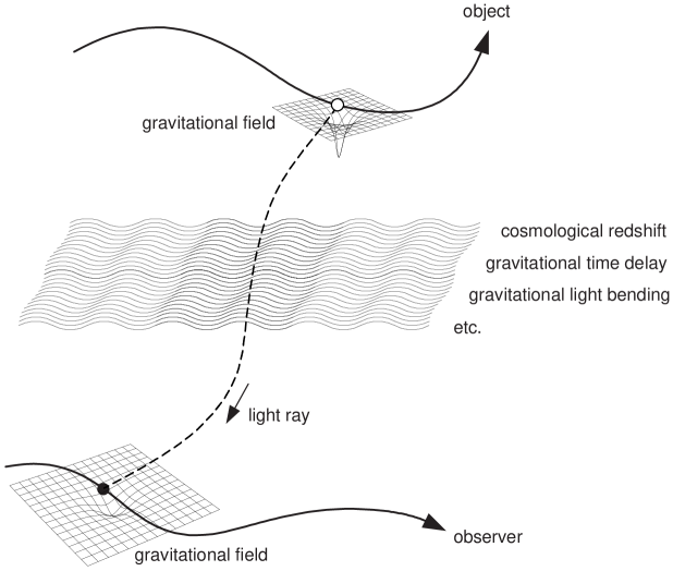
Figure 1: Whether a radial velocity is measured spectroscopically or geometrically, the relevant astronomical event consists of several parts: the motion of the observed object; the emission of an electromagnetic signal from the object, symbolised by the open circle; the propagation of the signal through space; the motion of the observer; and the reception of the signal by the observer, symbolised by the black dot (figure partially adapted from Klioner 2000a).

From these examples it should be clear that the naive concept of radial velocity, as the line-of-sight component of the stellar velocity vector measured by the Doppler shift of the spectral lines, is far too simplistic when aiming at accuracies much better than 1 km s^-1. To arrive at a consistent set of definitions applicable to the various classes of observations, it is necessary to consider all the phases of an astronomical event (Fig. 1). These include the motion of the star; the emission of a light signal from the star and its propagation to the observer through varying gravitational fields and possibly expanding space; the motion of the observer; and the reception and measurement of the signal by the observer. The observer has detailed knowledge only of the last two phases of the event (symbolised by the black dot in Fig. 1), while the interpretation of the previous phases requires additional assumptions or modelling. The result of a measurement should ideally be specified in a way that is neutral with respect to such interpretation. As we shall see (Sect. 5), this leads to the definition of barycentric radial-velocity measure as the desired result of a spectroscopic measurement. However, to relate this quantity to physical motion in even simple situations, a model is required which incorporates all phases of the event as illustrated in the figure. This, in turn, leads to the introduction of additional geometric quantities, viz. kinematic radial velocity and astrometric radial velocity (Sect. 4).

The remainder of this paper is organised as follows. Section 2 contains a preliminary heuristic discussion of the radial-velocity concept as such; the purpose is to point out the inadequacy and ambiguity of standard notions, without providing a solution. Section 3 then gives an overview of spectroscopic radial-velocity determinations, highlighting effects other than trivial stellar motion that influence the outcome of such measurements. The accurate meaning of the geometric and spectroscopic quantities is evaluated in the more technical Sections 4 and 5, leading up to the IAU resolutions, whose practical implications are considered in Sect. 6. Some unsolved issues, beyond the scope of the present definitions, are briefly discussed in Sect. 7. The Appendix contains the full text of the two IAU resolutions.

2 What is meant by ‘radial velocity’?

In this Section we examine the common notions of ‘radial velocity’ from a somewhat naive viewpoint, in order to highlight some of the difficulties associated with this apparently simple concept. Additional complications in the interpretation of spectroscopic shifts are discussed in Sect. 3.

2.1 Geometric concepts

The Encyclopedia of Astronomy and Astrophysics defines the radial velocity of a star as ‘the component of its motion along the line of sight of the observer’ (Latham 2001). The Explanatory Supplement to the Astronomical Almanac gives an alternative definition, ‘the rate of change of the distance to an object’ (Seidelmann 1992). Both agree with common notions about radial velocity, but are they equivalent? Let us start by examining this question in a purely classical framework, without the complications of relativity, but taking into account the finite speed of light ($c$).

In a Euclidean metric with origin at the solar-system barycentre and with $t$ denoting coordinate time, let $\@vec{r}_{\ast}(t)$ be the motion of the star, $\@vec{v}_{\ast}={\rm d}\@vec{r}_{\ast}/{\rm d}t$ its barycentric space velocity, $r_{\ast}=\left|\@vec{r}_{\ast}\right|$ the barycentric distance, and $\@vec{u}=\@vec{r}_{\ast}/r_{\ast}$ the barycentric direction to the star. Following the first of the two definitions quoted above, the radial velocity $v_{r}$ is the component of $\@vec{v}_{\ast}$ along $\@vec{u}$, or

$$v_{r}=\@vec{u}^{\prime}\@vec{v}_{\ast}\,,$$ (1)

where the prime (^′) denotes scalar multiplication of vectors. From $\@vec{r}_{\ast}=\@vec{u}r_{\ast}$ we can write the space velocity

$$\@vec{v}_{\ast}\equiv{\displaystyle\frac{{\rm d}\@vec{r}_{\ast}}{{\rm d}t}}={\displaystyle\frac{{\rm d}\@vec{u}}{{\rm d}t}}\,r_{\ast}+\@vec{u}\,{\displaystyle\frac{{\rm d}r_{\ast}}{{\rm d}t}}\,.$$ (2)

Taking the scalar product with $\@vec{u}$ we have, since $\@vec{u}^{\prime}\@vec{u}=1$ and $\@vec{u}^{\prime}({\rm d}\@vec{u}/{\rm d}t)=\frac{1}{2}{\rm d}(\@vec{u}^{\prime}\@vec{u})/{\rm d}t=0$,

$$\@vec{u}^{\prime}\@vec{v}_{\ast}={\displaystyle\frac{{\rm d}r_{\ast}}{{\rm d}t}}\,.$$ (3)

The right member apparently corresponds to the second definition quoted above. Comparing Eqs. (1) and (3) it therefore appears that we have proved the equivalence of the two definitions.

However, the situation is more complex when the finite speed of light is considered. The observation involves (at least) two different times, viz. the time of light emission at the star ($t_{\ast}$) and the time of light reception at the observer ($t_{\rm obs}$), cf. Fig. 1. The second definition, ‘the rate of change of the distance’, is in fact ambiguous because it is not specified which time is used to compute the time derivative. Clearly the $t$ in Eq. (3) must be the same as used in describing the motion of the star, $\@vec{r}_{\ast}(t)$, which should be independent of the observer and therefore corresponding to the time of light emission. However, when describing an observed phenomenon, such as a measurement of the line-of-sight velocity of a star, it is more natural to refer it to the time of light reception $t_{\rm obs}$.

The two instants $t_{\ast}$ and $t_{\rm obs}$ are related by the light-time equation, which for an observer at the solar-system barycentre (and ignoring gravitational time delay) is simply

$$r_{\ast}=c(t_{\rm obs}-t_{\ast})\,.$$ (4)

Depending on which $t$ is used to compute the ‘rate of change’ in the second definition, we obtain by means of the light-time equation two different expressions for $v_{r}$:

$$\left.\begin{array}[]{lllll}v_{r}^{\prime}&\equiv&{\displaystyle\frac{{\rm d}r_{\ast}}{{\rm d}t_{\ast}}}&=&c\left({\displaystyle\frac{{\rm d}t_{\rm obs}}{{\rm d}t_{\ast}}}-1\right)\\[16.0pt] v_{r}^{\prime\prime}&\equiv&{\displaystyle\frac{{\rm d}r_{\ast}}{{\rm d}t_{\rm obs}}}&=&c\left(1-{\displaystyle\frac{{\rm d}t_{\ast}}{{\rm d}t_{\rm obs}}}\right)\end{array}\quad\right\}$$ (5)

The difference, $v_{r}^{\prime}-v_{r}^{\prime\prime}=v_{r}^{\prime}v_{r}^{\prime\prime}/c\simeq v_{r}^{2}/c$, exceeds 1 m s^-1 for $|v_{r}|\ga 20$ km s^-1 and 100 m s^-1 for $|v_{r}|\ga 200$ km s^-1. Since relative velocities in our Galaxy are typically tens of km s^-1, and may reach several hundred km s^-1, the ambiguity has practical relevance in the context of precise stellar radial velocities.

It is seen from Eq. (5) that the ambiguity arises when the quantity ${\rm d}t_{\rm obs}/{\rm d}t_{\ast}$ is transformed into a velocity, i.e. when a model is used to interpret the data. ${\rm d}t_{\rm obs}/{\rm d}t_{\ast}$, on the other hand, is a direct, model-independent relation between the basic events of light emission and reception. From an observational viewpoint, we could therefore regard the dimensionless quantity ${\rm d}t_{\rm obs}/{\rm d}t_{\ast}$ as more fundamental than either $v_{r}^{\prime}$ or $v_{r}^{\prime\prime}$.

2.2 Doppler shift

The result of a spectroscopic line-shift measurement may be expressed by means of the dimensionless redshift variable

$$z=\frac{\lambda_{\rm obs}-\lambda_{0}}{\lambda_{0}}=\frac{\nu_{0}-\nu_{\rm obs}}{\nu_{\rm obs}}\,,$$ (6)

where $\lambda_{0}$ ($\nu_{0}$) is the rest-frame wavelength (frequency). The redshift is often converted to a conventional velocity using some standard formula, the simplest being

$$v_{r}^{(1)}=c\,\frac{\lambda_{\rm obs}-\lambda_{0}}{\lambda_{0}}=cz\,.$$ (7)

However, an alternative conversion is obtained by considering the relative shift in frequency rather than in wavelength, viz.:

$$v_{r}^{(2)}=c\,\frac{\nu_{0}-\nu_{\rm obs}}{\nu_{0}}=\frac{cz}{1+z}\,.$$ (8)

This last expression has traditionally been used in radio astronomy (e.g. Walker 1987), although the practice is discouraged due to the risk of confusion with the earlier expression (Contopoulos & Jappel 1974; Müller & Jappel 1977). $v_{r}^{(1)}$ is sometimes called the ‘optical velocity’ and $v_{r}^{(2)}$ the ‘radio velocity’ (Greisen et al. 2003).

For use with large velocities, the following formula is often recommended (e.g. Lang 1974):

$$v_{r}^{(3)}=c\,\frac{(1+z)^{2}-1}{(1+z)^{2}+1}\,.$$ (9)

The expression is derived from the special-relativistic Doppler formula by assuming purely radial motion (cf. below).

Thus we have at least three different conventions for transforming $z$ into $v_{r}$ that are more or less ‘standard’ in astronomy. From the series expansions

$$\left.\begin{array}[]{lll}v_{r}^{(1)}&=&cz\\[3.0pt] v_{r}^{(2)}&=&c\,(z-z^{2}+z^{3}-z^{4}+\cdots)\\[3.0pt] v_{r}^{(3)}&=&c\,(z-\frac{1}{2}z^{2}+\frac{1}{4}z^{4}-\cdots)\end{array}\quad\quad\right\}$$ (10)

it is seen that the differences between the three conventions are of second order ($cz^{2}\sim v_{r}^{2}/c$).

Equation (9) ignores the star’s transverse velocity ($v_{t}$). The complete Doppler formula from special relativity reads (Lang 1974):

$$1+z=\frac{1+v_{r}/c}{\sqrt{1-v^{2}/c^{2}}}\,,$$ (11)

where $v=(v_{r}^{2}+v_{t}^{2})^{1/2}$ is the total velocity relative the observer. Solving for $v_{r}$ and expanding in powers of $z$ and $u=v_{t}/c$ we obtain a fourth expression for $v_{r}$:

$$v_{r}^{(4)}=c\left[z-{\textstyle\frac{1}{2}}(z^{2}+u^{2})+{\textstyle\frac{1}{4}}zu^{2}+{\textstyle\frac{1}{4}}(z^{4}-u^{4})-\cdots\right].$$ (12)

Comparing with the third variant of Eq. (10) it is seen that the transverse Doppler effect is $\sim v_{t}^{2}/2c$, i.e. typically of a similar size as the differences among the expressions in Eq. (10).

Thus, various conventions exist for converting the observed Doppler shift into a radial velocity; the differences are of order $v^{2}/c$, exceeding 1 m s^-1 for normal galactic stellar velocities and 100 m s^-1 for high-velocity stars. Within the framework of special relativity (thus ignoring the many other effects discussed below), a ‘rigorous’ transformation from $z$ to $v_{r}$ is possible, but only if the transverse velocity of the star is also known.

2.3 Astrometric determination or radial motion

Astrometry specialises in measuring the directions to objects, and in particular the directional changes caused by the motions of the object (proper motion) and observer (parallax). Although such measurements primarily yield the distances and transverse velocities of the objects, they are in principle sensitive also to the radial motion of the objects through various second-order effects. Although the principles have been known for a long time, it is only with the high accuracies realised with space techniques that astrometry has become a practical possibility for radial-velocity measurements.

Different methods exist for the determination of astrometric stellar radial velocities (Dravins et al. 1999). The most direct method, measuring the rate of parallax change as a star approaches or recedes, is still beyond realised accuracies (e.g., even for the nearby high-velocity Barnard’s star, the expected parallax rate is only 34 $\mu$as yr^-1), although it is expected to become measurable in the foreseeable future. Another method utilises that a star’s proper motion changes as a result of its changing distance from the Sun (‘perspective acceleration’). By combining high-accuracy proper motions with measurements of stellar positions at different epochs, radial-velocity values have so far been determined for some 20 stars, though only with modest accuracies (typically a few tens of km s^-1; Dravins et al. 1999). However, a third method, applicable to nearby moving clusters such as the Hyades, whose stars share the same (average) velocity vector, already permits accuracies on the sub-km s^-1 level, and for several classes of stars has yielded better data than have been possible to achieve spectroscopically. Here, parallaxes and proper motions are combined to determine the apparent secular expansion or contraction of the angle subtended by a cluster, as it is approaching or receding. Using data from the Hipparcos satellite mission, more than a thousand stars have already been thus studied (Madsen et al. 2002), a number to be increased when data from future astrometry missions become available.

These methods are all based on the same general principle: let $\theta$ be the angular size of an object (the Earth’s orbit as seen from the star, the distance travelled by the star in a given time, or the size of a stellar cluster) and $r$ its distance; then the assumption is that $r\theta=$ constant, from which $\dot{r}=-r\dot{\theta}/\theta$. While the principle is simple enough, the question still remains whether the derivative ($\dot{\phantom{r}}$) should be taken with respect to the time of observation, or the time of light emission. Thus, also the concept of astrometric radial velocities needs a more precise definition.

3 Limitations of spectroscopic radial-velocity measurements

In this Section we highlight the various issues that may limit the achievable accuracy in stellar radial velocities, as deduced from spectroscopic observations.

3.1 Gravitational redshifts

The gravitational potential induced by a star’s mass causes redshifts of all photons leaving its vicinity. Across the Hertzsprung–Russell diagram, the gravitational redshifts change by three orders of magnitude between white dwarfs (some 30 km s^-1) and supergiants (some 30 m s^-1). This gravitational redshift $v_{\rm grav}=GM/rc$ diminishes with distance from the stellar centre as $r^{-1}$. For the Sun, the value is 636.5 m s^-1 for light escaping from the solar photosphere ($r=R_{\odot}$) to infinity, and 633.5 m s^-1 for light intercepted at the Earth’s mean distance from the Sun ($r=215R_{\odot}$). A solar spectral line instead formed at chromospheric heights (30 Mm, say; $r=1.04R_{\odot}$) will have this redshift decreased by some 20 m s^-1, and a coronal line by perhaps 100 m s^-1.

For other stars, the shift scales as $(M/M_{\odot})(R/R_{\odot})^{-1}$, or as $(g/g_{\odot})(R/R_{\odot})$, where $g$ is the surface gravity. Since $R$ and $M$ can rarely be estimated to better than $\sim$ 5% for single stars (Andersen 1991), while spectroscopic determinations of $\log g$ have much larger uncertainties (Lebreton 2000), it is normally not possible to compute the gravitational redshift to better than 50 m s^-1 for individual single stars.

3.2 Effects inside stellar atmospheres

It is well known that photospheric absorption lines in the solar spectrum are blueshifted by about 400 m s^-1 (after correction for the known gravitational redshift) as a result of convective motions in the solar atmosphere. In the photospheric granulation, hot (bright) and rising (blueshifted) convective elements contribute more photons than the cooler (darker) and sinking (redshifted) gas, thus causing a net blueshift of the absorption lines (Dravins 1982; Allende Prieto & García López 1998). Detailed modelling of stellar atmospheres involving 3-dimensional and time-dependent hydrodynamics is capable of producing synthetic spectral lines whose intensity profiles and patterns of wavelength displacements closely match observations for at least solar-type stars (e.g. Asplund et al. 2000; Allende Prieto et al. 2002). For main-sequence stars, the predicted convective blueshifts range between approximately 1000 m s^-1 for F-type stars and 200 m s^-1 for cooler K-types.

The shift is however not the same for all the lines in a spectrum. The precise amount of shift depends on the strength of the absorption line (and hence on the stellar metallicity), since different lines are formed at different atmospheric depths and thus experience different granulation contrasts. For the Sun such (observed and modelled) differential shifts between differently strong lines in the visual amount to some 200 m s^-1, but reach 1000 m s^-1 for the hotter F-type star Procyon (Allende Prieto et al. 2002). The shifts further depend on excitation potential and ionisation level (due to different conditions of line formation), and on wavelength region (due to varying granulation contrast). Actually, in some wavelength regions, where the lines may originate in atmospheric layers characterised by convective overshoot (with an inverted velocity/temperature correlation), the lineshifts may change sign to become convective redshifts. For the Sun this can be observed in cores of very strong lines in the optical or generally in the far ultraviolet (Samain 1991).

Line profiles are also asymmetric, making the determination of accurate lineshifts a matter of convention – where in the line should the shift be measured? Asymmetries are caused not only by convective motions on the stellar surface but also by asymmetric emission and/or absorption components (e.g., due to chromospheric emission or stellar-wind absorption), by microscopic processes causing wavelength shifts on the atomic level (e.g., pressure shifts), or macroscopic circumstances (e.g., gravitational redshift). Further complications enter for pulsating stars, those with expanding atmospheres, or such with deviant isotopic compositions.

Since many physical effects thus contribute to the observed wavelength shifts (e.g. Dravins 2003), it is not possible to deduce an accurate centre-of-mass motion simply from the observed differences between wavelengths in the source and those measured in the laboratory.

3.3 The role of standard stars

Radial-velocity standards, with a supposedly known ‘true’ velocity, have long been used as objects against which to calibrate observations of other stars. Indeed, a goal of the IAU Working Group on Radial Velocity Standard Stars has been ‘to provide a list of such standard stars whose velocities are known with an accuracy of 100 m s^-1.’ Overviews of the work by this and other groups are in Stefanik et al. (1999); Udry et al. (1999); Fekel (1999), and in various triennial reports from IAU Commission 30 on radial velocities, published in the IAU Transactions (e.g. Bergeron 1994; Andersen 1999; Rickman 2001).

In practical application, however, a number of dependences on the 0.5 km s^-1 level have been found, in particular on the stellar colour index, differences among different radial-velocity instruments, between different spectrum correlation masks applied on the same stellar spectrum, etc. The best agreement is normally found for stars of spectral type close to that of the Sun – naturally so, since the instruments and data reductions are normally calibrated against the solar spectrum e.g. as reflected off minor planets, whose motions are accurately known through other methods, and the procedures set up to produce consistent results at least for such a solar spectrum.

However, not even very elaborate calibrations are likely to produce any ‘true’ standards to a much better precision than 0.5 (or, perhaps, 0.3) km s^-1, unless a detailed physical model of the observed star is developed. The reason is simply the physical nature of stellar spectra and the practical impossibility to obtain noise-free measurements. Apart from the physical effects of stellar surface convection and gravitational redshifts mentioned above, the wavelengths of stellar spectral lines depend on, i.a., factors such as the stellar rotation rate, the angle under which the stellar rotation axis is observed, the phase in a possible magnetic stellar activity cycle, and the spectral resolution and instrumental profile of the observer’s instrument. Here, we give examples of such effects that are likely to limit the ultimate achievable precision for radial-velocity standard-stars to levels not much better than 0.5 km s^-1:

3.3.1 Effects of stellar rotation

The influence of stellar rotation has been realised, especially for earlier-type stars with their often rapid rotation (Andersen & Nordström 1983; Verschueren & David 1999; Griffin et al. 2000). The effects caused by the mismatch between a spectrum template for a slow-rotation star and a rapidly rotating A-type star may exceed 1 km s^-1 (Verschueren & David 1999). The origin of these effects is the rotational line-broadening and the ensuing blending of spectral lines, significant when a given star is observed equator-on, but disappearing when viewed pole-on.

Even very modest rotational velocities in sharp-lined late-type stars may cause significant wavelength displacements of the spectral-line bottoms and other parts of the line profiles used for radial-velocity determinations. Naively, one might expect that increased stellar rotation would merely smear out the line profiles and perhaps straighten out the bisectors which describe the line asymmetry. Actually, for more rapid rotation, when the asymmetric line components originating near the stellar limbs begin to affect the wings of the profile integrated over the stellar disk, the line asymmetries may become enhanced. This phenomenon was suggested by Gray & Toner (1985) and by Gray (1986) and studied in more detail for a simulated rapidly rotating Sun by Smith et al. (1987). Detailed line profile calculations from hydrodynamic model atmospheres for stars of different types (Dravins & Nordlund 1990) show that this effect may easily displace photospheric line-bottoms by a few hundred m s^-1 already in solar-type stars rotating with $V\sin i$ less than 10 km s^-1. Also, stars may rotate not as rigid bodies, and rotation may be differential with respect to stellar latitude, atmospheric height, or between magnetic and non-magnetic elements. The existence of differential rotation is suggested both from studies of starspots (e.g., Weber & Strassmeier 2001; Collier Cameron et al. 2002), and from analyses of line profiles (Reiners et al. 2001).

3.3.2 Effects of stellar activity cycles

On levels of perhaps 10–100 m s^-1, at least cooler stars undergo apparent radial-velocity variations during a stellar activity cycle, when differently large fractions of the stellar surface are covered by active regions with magnetically ‘disturbed’ granulation (e.g., Gray et al. 1996). Magnetic flux that becomes entangled among the convective features limits the sizes and the temperature and velocity amplitudes to which these features develop. For solar observations, see Spruit et al. (1990,  their Fig. 1) and Schmidt et al. (1988); for theory, see Bercik et al. (1998). The resulting spectral line asymmetries are changed in the sense of smaller asymmetries and smaller wavelength shifts in the active regions (e.g. Immerschitt & Schröter 1989; Brandt & Solanki 1990,  and references therein).

Livingston et al. (1999) followed the full-disk asymmetries of Fe i lines during a full 11-year solar activity cycle, finding cyclic variations in the line asymmetry with an amplitude of about 20 m s^-1; presumably the corresponding absolute shifts are (at least) of a similar size. Indeed, variations on this order can be predicted from spatially resolved observations of line profiles in active regions, weighted with the cyclically changing area coverage of active regions during an activity cycle. The effects can be expected to increase (to perhaps 50 m s^-1) for younger and chromospherically more active stars, e.g., F- and G-type ones in the Hyades (Saar & Donahue 1997).

Since the amount of convective lineshift differs among different types of spectral lines and between different spectral regions, also the activity-induced changes in this shift must be expected to differ. While the identification of such differences could be important to find lines whose sensitivity to stellar activity is smaller (thus being better diagnostics for exoplanet signatures) or greater (being better diagnostics for magnetic activity), such data are not yet available (and may indeed require a stringent definition of the radial-velocity measure to permit intercomparisons between observations at different epochs).

Besides these cyclic changes, there are shorter-term fluctuations (on a level of perhaps 20–30 m s^-1) in the apparent radial velocity of stars, which often are greater in stars with enhanced chromospheric activity. Presumably, this reflects the evolution and changing area coverages of active regions (e.g. Saar et al. 1998; Saar & Fischer 2000; Santos et al. 2000).

3.3.3 Effects caused by starspots and surface inhomogeneities

Greater effects are present in spotted stars whose photometric variability indicates the presence of dark spots across the stellar surface. The amplitude of variations expected from photometrically dark spots is on the order of 5 m s^-1 for solar-age G-type stars, increasing to perhaps 30–50 m s^-1 for younger and more active stars (Saar & Donahue 1997; Hatzes 2002). In more heavily spotted stars (such already classically classified as variables), the technique of Doppler imaging exploits the variability of spectral-line profiles to reconstruct stellar surface maps (e.g., Piskunov et al. 1990), but obviously any more accurate deduction of the radial motion of the stellar centre-of-mass from the distorted spectral lines is not a straightforward task.

Surface inhomogeneities causing such line distortions need not be connected to photometrically dark (or bright) spots, but could be chemical inhomogeneities across the stellar surface (with locally different line-strengths) or just patches of granulation with different structure (Toner & Gray 1988).

3.3.4 Effects caused by the finite number of granules

Even the spectrum of a hypothetical spot-less and non-rotating star with precisely known physical and chemical properties will probably still not be sufficiently stable to serve as a ‘standard’ on our intended levels of accuracy. One reason is the finite number of convective features (granules) across the stellar surface. For the Sun, a granule diameter is on the order of 1000 km, and there exist, at any one time, on the order of $10^{6}$ such granules on the visible solar disk. The spectrum of integrated sunlight is made up as the sum of all these contributions: to make an order-of-magnitude estimate, we note that each granule has a typical velocity amplitude of 1–2 km s^-1. Assuming that they all evolve at random, the apparent velocity amplitude in the average will be this number divided by the square root of $10^{6}$, or 1–2 m s^-1. This ‘astrophysical noise’ caused by the finite number of granules is a quantity that is becoming measurable also in solar-type stars in the form of an excess of the power spectrum of spectral-line variability at temporal frequencies of some mHz, corresponding to granular lifetimes on the order of ten minutes (Kjeldsen et al. 1999). Although it can also be modelled theoretically (e.g. Trampedach et al. 1998), such modelling can only predict the power spectrum and other statistical properties, not the instantaneous state of any star.

The number of granules across the surfaces of stars of other spectral types may be significantly smaller than for the Sun, and the resulting ‘random’ variability correspondingly higher. For supergiants, it has been suggested than only a very small number of convective elements (perhaps only a few tens) coexist at any given time, but even a star with $10^{4}$ granules would show radial-velocity flickering an order of magnitude greater than the Sun.

The effects are qualitatively similar for other types of statistically stable structures across stellar surfaces, e.g. p-mode oscillations, where various surface regions on the star are moving with varying vertical velocities. Since their averaging across the star does not fully cancel, they are detectable as lineshift variations on a level of several m s^-1 (e.g. Hatzes 1996; Bedding et al. 2001; Frandsen et al. 2002), demonstrating another application of precise radial-velocity measurements, as well as the limitations to stellar wavelength stability.

3.3.5 Effects caused by exoplanets

Intrinsically stable stars may show variability on the 10–100 m s^-1 level induced by orbiting exoplanets. Of course, this is a true radial-velocity variation, but it practically limits the selection of such stars as radial-velocity ‘standards’, since their use on the m s^-1 level would require detailed ephemerides for their various exoplanets. It can be noted that 51 Peg used to be a radial-velocity standard star!

3.3.6 Effects of instrumental resolution

A different type of wavelength displacements is introduced by the observing apparatus, in effect convolving the pristine stellar spectrum with the spectrometer instrumental profile. Since all stellar spectral lines are asymmetric to some extent, their convolution with even a perfectly symmetric instrumental profile of an ideal instrument produces a different asymmetry, and a different wavelength position e.g. of the line-bottoms. Quantitative calculations demonstrate how such effects reach 50 m s^-1 and more, even for high-resolution instruments (Bray & Loughhead 1978; Dravins & Nordlund 1990). Although this is ‘only’ a practical limitation which, in principle, could be corrected for if full information of the instrumental response were available, this is not likely to be possible in practice. For example, differences of many tens of m s^-1 in measured lineshifts may result between spectrometers with identical spectral resolutions (measured as full width at half-maximum), but which differ only in their amounts of diffuse scattered light (Dravins 1987). Of course, even greater lineshifts could be caused by asymmetric instrumental profiles. Instrumental effects in spectroscopy are reviewed by Dravins (1994) while methods for calibrating instrumental profiles are discussed by, e.g., Valenti et al. (1995) and Endl et al. (2000).

3.3.7 Effects of instrumental design

For observational modes not involving analyses of highly resolved line profiles, but rather statistical functions such as the cross-correlation between spectral templates, a series of other instrumental effects may intermix with stellar ones. For example, if a detector/template combination predominantly measures a signal from the blue spectral region, it may be expected to record a somewhat greater spectral blueshift in cool stars since convective blueshifts generally increase at shorter wavelengths (where a given temperature contrast in surface convection causes a relatively greater brightness contrast). A red-sensitive system may give the opposite bias, unless it is sensitive into the infrared, where the generally smaller stellar atmospheric opacities make the deeper layers visible, with perhaps greater convective amplitudes.

3.3.8 Conclusions about spectroscopic ‘standard’ stars

Physical and instrumental effects, such as those listed above (and others, such as errors in laboratory wavelengths), imply that there most probably do not exist any stars whose spectral features could serve as a real standard on precision levels better than perhaps 300 m s^-1. Of course, for poorer precisions – perhaps around 0.5 km s^-1 – various standard sources, including the solar spectrum, may continue to be used as before. However, in order to deduce true velocities to high accuracy, all spectral observations – of ‘standard’ stars and others – must undergo a detailed physical modelling of their emitted spectrum, and of its recording process.

3.3.9 Possible future astrometric standard stars

The recently realised accurate determination of stellar radial motions through astrometric measurements opens the possibility of having also radial-velocity standards determined independent of spectroscopy. While the ultimate limitations in thus obtainable accuracies have not yet been explored (e.g., what is measured in astrometry is the photocentre of the normally unresolved stellar disk, whose coordinates may be displaced by starspots or other features) there appear to be no known effects that in principle would hinder such measurements to better than 100 m s^-1 (or even 10 m s^-1), at least for some nearby stars. This will require astrometric accuracies on the microarcsecond level, and possibly extended periods of observations, but these are expected to be reachable in future space astrometry missions (Dravins et al. 1999).

3.4 Conclusions

From the above discussion it is clear that numerous effects may influence the precise amount of spectral-line displacements. Among these, only local effects near the observer (i.e., within the [inner] solar system) can be reliably calculated and compensated for. In particular, these depend on the motion and gravitational potential of the observer relative to the desired reference frame, normally the solar-system barycentre.

Therefore, spectroscopic methods will not be able, in any foreseeable future, to provide values of stellar radial motion with ‘absolute’ accuracies even approaching our aim of 1 m s^-1. Of course, this does not preclude that measurement precisions (in the sense of their reproducibility) may be much better and permit the detection of very small variations in the radial velocity of an object (whose exact amount of physical motion will remain unknown) in the course of searching for, e.g., stellar oscillations or orbiting exoplanets. In order to enable further progress in the many fields of radial-velocity studies, it seems however that more stringent accuracy targets have to be defined, so that future observational and theoretical studies have clear goals to aim at.

Astrometric radial velocities do not appear to have the same types of limitations as those deduced from spectroscopic shifts, and more lend themselves to definitions that can be transformed to ‘absolute’ physical velocities. These, however, must be stringently defined since different plausible definitions differ by much more than our desired accuracies.

4 Kinematic and astrometric radial velocity

We will now more thoroughly scrutinise the various geometric effects entering the concept of ‘radial velocity’, aiming at definitions that are consistent at an accuracy level of 1 m s^-1. This requires first that a system of temporal and spatial coordinates is adopted; then that the relevant parts of the astronomical event (Fig. 1) are modelled in this system, consistent with general relativity at the appropriate accuracy level; and finally that suitable conventions are proposed for the parameterisation of the event.

The modelling of astrometric observations within a general-relativistic framework has been treated in textbooks such as Murray (1983), Soffel (1989) and Brumberg (1991), and various aspects of it have been dealt with in several papers (e.g. Stumpff 1985; Backer & Hellings 1986; Klioner & Kopeikin 1992; Klioner 2000b, 2003). Much of the mathematical development in this and the next Section is directly based on these treatments, but adapted in order to present a coherent background for the definition and explanation of the radial-velocity concepts.

4.1 Coordinate system (BCRS)

Subsequently, $t$ and $\@vec{r}\equiv(x,y,z)$ denote coordinates in the Barycentric Celestial Reference System (BCRS) adopted by the IAU 24th General Assembly (Rickman 2001) and discussed by Brumberg & Groten (2001). The temporal coordinate $t$ is known as the Barycentric Coordinate Time (TCB). The BCRS is a well-defined relativistic 4-dimensional coordinate system suitable for accurate modelling of motions and events within the solar system. However, it also serves as a quasi-Euclidean reference frame for the motions of nearby stars and of more distant objects, thanks to some useful properties: it is asymptotically flat (Euclidean) at great distances from the Sun; the directions of its axes are fixed with respect to very distant extragalactic objects; and the origin at the solar-system barycentre provides a local frame in which nearby (single) stars appear to be non-accelerated, as they experience practically the same galactic acceleration as the solar system. The axes are aligned with the celestial system of right ascension and declination as realised, for example, by the Hipparcos and Tycho Catalogues (ESA 1997).

4.2 The light-time equation

As emphasised in Sect. 2.1, the relation between the events of light emission and light reception is fundamental for describing the astronomical event resulting in a geometric or spectroscopic observation. The two events are connected by the light-time equation, from which the required spatial and temporal transformations may be derived.

In the BCRS, let $\@vec{r}_{\ast}(t)$ describe the motion of the star and $\@vec{r}_{\rm obs}(t)$ that of the observer. Assume that a light signal is emitted from the star at time $t_{\ast}$, when the star is at the spatial coordinate $\@vec{r}_{\ast}\equiv\@vec{r}_{\ast}(t_{\ast})$ and its coordinate velocity is $\@vec{v}_{\ast}\equiv(\mbox{d}\@vec{r}_{\ast}/\mbox{d}t)_{t=t_{\ast}}$. Assume, furthermore, that the same light signal is received by the observer at time $t_{\rm obs}$, when the observer is at the spatial coordinate $\@vec{r}_{\rm obs}\equiv\@vec{r}_{\rm obs}(t_{\rm obs})$ and its coordinate velocity is $\@vec{v}_{\rm obs}\equiv(\mbox{d}\@vec{r}_{\rm obs}/\mbox{d}t)_{t=t_{\rm obs}}$. The light-time equation can now be written

$$t_{\rm obs}-t_{\ast}=c^{-1}\left|\@vec{r}_{\ast}-\@vec{r}_{\rm obs}\right|+\gamma\left(t_{\ast},\@vec{r}_{\ast};t_{\rm obs},\@vec{r}_{\rm obs}\right)\,.$$ (13)

Here, $c=299\,792\,458$ m s^-1 is the conventional speed of light, $|\,|$ denotes the usual (Euclidean) vector norm, and $\gamma$ is the relativistic delay of the signal along the path of propagation from star to observer. The delay term is required to take into account that the coordinate speed of light in the presence of a gravitational field is less than $c$ in the adopted metric, so that the first term in Eq. (13) gives too small a value for the light travel time. For present purposes it is sufficient to describe the gravitational field by means of the total Newtonian potential $\Phi(\@vec{r})$ relative to the BCRS. For instance, the gravitational field of the solar system is adequately described by $\Phi(\@vec{r})=G\sum_{i}M_{i}|\@vec{r}-\@vec{r}_{i}|^{-1}$, where $G$ is the gravitational constant, and the sum is taken over the different solar-system bodies having (point) masses $M_{i}$ located at coordinates $\@vec{r}_{i}$. To first order in $c^{-2}$, the coordinate speed of light in the BCRS metric is given by $|\mbox{d}\@vec{r}/\mbox{d}t|=c(1-2\Phi/c^{2})$. The time delay per unit length is therefore $2\Phi/c^{3}$. Integrating this quantity along the light path (which for this calculation can be taken to be a straight line in the BCRS coordinates) gives

$$\gamma=\sum_{i}\frac{2GM_{i}}{c^{3}}\,\ln\left(\frac{\@vec{k}^{\prime}(\@vec{r}_{\ast}-\@vec{r}_{i})+|\@vec{r}_{\ast}-\@vec{r}_{i}|}{\@vec{k}^{\prime}(\@vec{r}_{\rm obs}-\@vec{r}_{i})+|\@vec{r}_{\rm obs}-\@vec{r}_{i}|}\right)\,.$$ (14)

$\@vec{k}$ is the coordinate direction from the observer to the star,

$$\@vec{k}=\left|\@vec{r}_{\ast}-\@vec{r}_{\rm obs}\right|^{-1}\left(\@vec{r}_{\ast}-\@vec{r}_{\rm obs}\right)\,.$$ (15)

Subsequently, we shall mainly consider the gravitational field of the Sun (index $=\odot$), for which $2GM_{\odot}c^{-3}\simeq 9.85\leavevmode\nobreak\ \mu$s. For objects as distant as the stars we can neglect $\@vec{r}_{\odot}$ compared with $\@vec{r}_{\ast}$ in the numerator of the argument to the logarithm in Eq. (14). Moreover, $\@vec{k}$ is practically parallel with $\@vec{r}_{\ast}$, so the numerator becomes simply $2r_{\ast}$, where $r_{\ast}=|\@vec{r}_{\ast}|$. (The error introduced by this approximation is $<10^{-16}$ s for $r_{\ast}>1$ pc.) The denominator varies depending on the relative positions of the Sun, observer and star, but is typically of the order of the astronomical unit ($A$) for an observer on the Earth. Thus $\gamma\sim(10\leavevmode\nobreak\ \mu\mbox{s})\ln(2r_{\ast}/A)$, or $\sim 100\leavevmode\nobreak\ \mu$s for the nearest stars, $\sim 200\leavevmode\nobreak\ \mu$s at $r_{\ast}=10$ kpc, and $\sim 300\leavevmode\nobreak\ \mu$s for objects at cosmological distances. This slowly varying delay of a few hundred microseconds suffered by the light while propagating from the star to the solar system is generally ignored. Indeed, it would hardly make sense to try to evaluate it, since the gravitational delays caused by other bodies (in particular by the star itself) are not included.

However, there is also a rapidly varying part of $\gamma$ in Eq. (14), caused by the motion of the observer with respect to the Sun. In order to separate the rapidly varying part of the delay from the (uninteresting) long-range delay, we write

$$\gamma=\gamma_{\ast}-\sum_{i}\frac{2GM_{i}}{c^{3}}\,\ln\!\left(\frac{\@vec{k}{{}^{\prime}}(\@vec{r}_{\rm obs}-\@vec{r}_{i})+|\@vec{r}_{\rm obs}-\@vec{r}_{i}|}{A}\right)\!,$$ (16)

where

$$\gamma_{\ast}=2G\Big{(}{\textstyle\sum_{i}M_{i}}\Big{)}c^{-3}\,\ln\!\left(\frac{2r_{\ast}}{A}\right)$$ (17)

is practically a constant for the star (cf. below). Clearly any constant length could have served instead of $A$ to separate the terms in Eq. (16). Using the astronomical unit for this purpose is just an arbitrary convention.

From the light-time equation we can now determine the relation between the coordinate time interval $\mbox{d}t_{\ast}$ (e.g. representing one period of emitted radiation) and $\mbox{d}t_{\rm obs}$ (the corresponding period of coordinate time at the observer). Writing $|\@vec{r}_{\ast}-\@vec{r}_{\rm obs}|=\@vec{k}{{}^{\prime}}(\@vec{r}_{\ast}-\@vec{r}_{\rm obs})$ we have

$$\mbox{d}t_{\rm obs}-\mbox{d}t_{\ast}=\@vec{k}{{}^{\prime}}(\mbox{d}\@vec{r}_{\ast}-\mbox{d}\@vec{r}_{\rm obs})c^{-1}+\mbox{d}\gamma\,,$$ (18)

from which

$$\frac{\mbox{d}t_{\ast}}{\mbox{d}t_{\rm obs}}=\frac{1+\@vec{k}{{}^{\prime}}\@vec{v}_{\rm obs}\,c^{-1}-\mbox{d}\gamma/\mbox{d}t_{\rm obs}}{1+\@vec{k}{{}^{\prime}}\@vec{v}_{\ast}\,c^{-1}}\,.$$ (19)

From Eqs. (16)–(17) it follows that $\mbox{d}\gamma/\mbox{d}t_{\rm obs}$ is the sum of two terms, the first of which $\simeq(10\leavevmode\nobreak\ \mu\mbox{s})\rho/r_{\ast}$, where $\rho=\mbox{d}r_{\ast}/\mbox{d}t_{\rm B}$ is the astrometric radial velocity of the star defined below (Sect. 4.5). For $|\rho|<c$ and $r_{\ast}>1$ pc this term is $<10^{-13}$ and therefore negligible. The second term can be evaluated e.g. for an observer in circular orbit (at 1 AU) around the Sun. It reaches a maximum value of $<10^{-9}$ when the observer is behind the Sun so that the light ray from the object just grazes the solar limb. The simple expression

$$\frac{\mbox{d}t_{\ast}}{\mbox{d}t_{\rm obs}}=\frac{1+\@vec{k}{{}^{\prime}}\@vec{v}_{\rm obs}\,c^{-1}}{1+\@vec{k}{{}^{\prime}}\@vec{v}_{\ast}\,c^{-1}}$$ (20)

is therefore always good enough to a relative accuracy better than $10^{-9}$ ($<0.3$ m s^-1 in velocity).

4.3 Barycentric time of light arrival

Since distances to objects beyond the solar system are generally not known very accurately, it would be inconvenient to use the time coordinate $t_{\ast}$ for describing observations of phenomena that occur at such great distances. Instead, it is customary to relate the observed events to the time scale of the observer. For very accurate timing, e.g. as required in pulsar observations, one must take into account both the geometrical (Rømer) delay associated with the observer’s motion around the solar-system barycentre, and the relativistic (Shapiro) delay caused by the gravitational field of bodies in the solar system.

We define the barycentric time of light arrival as

$$t_{\rm B}=t_{\ast}+r_{\ast}\,c^{-1}+\gamma_{\ast}\,,$$ (21)

where $\gamma_{\ast}$ is given by Eq. (17). That is, $t_{\rm B}$ is the time of light emission delayed by the nominal propagation time to the barycentre ($r_{\ast}/c$) plus that part of the relativistic delay which is independent of the observer. By means of Eqs. (14) and (16) we find that the barycentric time of light arrival becomes

$$t_{\rm B} = t_{\rm obs}+(r_{\ast}-R)\,c^{-1}$$ (22)

$$+\sum_{i}\frac{2GM_{i}}{c^{3}}\,\ln\left[\frac{\@vec{k}{{}^{\prime}}(\@vec{r}_{\rm obs}-\@vec{r}_{i})+|\@vec{r}_{\rm obs}-\@vec{r}_{i}|}{A}\right]\,,$$

where $R=|\@vec{r}_{\ast}-\@vec{r}_{\rm obs}|$ is the topocentric coordinate distance to the star. With $\@vec{r}_{\ast}=\@vec{u}r_{\ast}$, where $\@vec{u}$ is the barycentric coordinate direction to the star, the Rømer delay can be expanded to give

$$(r_{\ast}-R)\,c^{-1}\simeq\frac{\@vec{u}{{}^{\prime}}\@vec{r}_{\rm obs}}{c}-\frac{|\@vec{u}\times\@vec{r}_{\rm obs}|^{2}}{2cr_{\ast}}+\frac{(\@vec{u}{{}^{\prime}}\@vec{r}_{\rm obs})^{3}}{2cr_{\ast}^{2}}\,.$$ (23)

For $r_{\ast}>1$ pc and $r_{\rm obs}\sim 1$ AU the maximum amplitudes of the three terms are $\simeq 500$ s, $1$ ms, and $4$ ns, respectively; neglected terms are of order $<10^{-13}$ s.

While Eq. (21) formally defines the barycentric time of light arrival, it is clear that Eqs. (22)–(23) must in practice be used to calculate it for any given observation. In principle this also requires that the distance $r_{\ast}$ is known, but only to a moderate precision. In many practical situations, the curvature terms in Eq. (23) [depending on $r_{\ast}^{-1}$ and $r_{\ast}^{-2}$] can be neglected.

4.4 Definition of kinematic parameters

Within the BCRS we define the kinematic parameters of a star to be its coordinate $\@vec{r}_{\ast}$ at time $t_{\ast}$, and the instantaneous coordinate velocity at the same instant, $v_{\ast}=\mbox{d}\@vec{r}_{\ast}/\mbox{d}t|_{t=t_{\ast}}$. In a time interval around $t_{\ast}$ we have

$$\@vec{r}_{\ast}(t)=\@vec{r}_{\ast}(t_{\ast})+(t-t_{\ast})\@vec{v}_{\ast}+{\cal O}(t-t_{\ast})^{2}\,.$$ (24)

The six components of the phase-space vector $(\@vec{r}_{\ast},\@vec{v}_{\ast})$ are the relevant elements for studies of galactic kinematics and dynamics, for example integration of galactic orbits (after transformation to a galactocentric system).

We define the kinematic radial velocity as the component of $\@vec{v}_{\ast}$ along the barycentric direction $\@vec{u}=\@vec{r}_{\ast}r_{\ast}^{-1}$:

$$v_{r}=\@vec{u}{{}^{\prime}}\@vec{v}_{\ast}\,.$$ (25)

The perpendicular component of the coordinate velocity is the kinematic tangential velocity, $\@vec{v}_{t}=\@vec{v}_{\ast}-\@vec{u}v_{r}$. The kinematic radial and tangential velocities are equivalent to the ‘true’ radial and tangential velocities introduced by Klioner (2000b).

4.5 Definition of astrometric parameters

The six components of $(\@vec{r}_{\ast},\@vec{v}_{\ast})$ are not directly observable but can in principle be derived from astrometric observations of the star. There is consequently an equivalent set of six astrometric parameters, which we now define. Following the discussion in Sect. 4.3, the astrometric parameters are considered as functions of $t_{\rm B}$. Writing the barycentric coordinate of the star as

$$\@vec{r}_{\ast}=\@vec{u}r_{\ast}$$ (26)

we define the celestial coordinates $(\alpha,\delta)$ of the star at the epoch $t_{\rm B}$ by means of the components of the unit vector $\@vec{u}$ in the BCRS. This gives the first two astrometric parameters. The third one is parallax, which we define as

$$\pi=\frac{A}{r_{\ast}}\,$$ (27)

(cf. Klioner 2000b). The rate of change of the barycentric direction is the proper-motion vector,

$$\@vec{\mu}=\frac{\mbox{d}\@vec{u}}{\mbox{d}t_{\rm B}}\,,$$ (28)

from which the proper motion components $\mu_{\alpha*}=\dot{\alpha}\cos\delta$ and $\mu_{\delta}=\dot{\delta}$ follow (the dot signifies differentiation with respect to $t_{\rm B}$). These five parameters are practically identical to the standard astrometric parameters used, for instance, in the Hipparcos Catalogue. The sixth astrometric parameter is the rate of change in barycentric coordinate distance, which we call the astrometric radial velocity:

$$\rho=\frac{\mbox{d}r_{\ast}}{\mbox{d}t_{\rm B}}\,.$$ (29)

The term is motivated because of the exact analogy with the definition of the (astrometric) proper motion in Eq. (28). Observationally, the astrometric radial velocity can in principle be determined e.g. from the secular change in parallax, $\rho=\Delta(A/\pi)/\Delta t_{\rm B}$ (Dravins et al. 1999). The vector $\@vec{\mu}r_{\ast}$ may be called the astrometric tangential velocity. The astrometric radial and tangential velocities are equivalent to the ‘apparent’ radial and tangential velocities introduced by Klioner (2000b).

It should be noted that the astrometric radial velocity is conceptually quite different from the spectroscopic radial-velocity measure to be defined in Sect. 5. The astrometric radial velocity refers to the variation of the coordinates of the source, and therefore depends on the chosen coordinate system and time scale. By contrast, the outcome of a spectroscopic observation is a directly measurable quantity and therefore independent of coordinate systems.

4.6 Transformation between kinematic and astrometric parameters

The barycentric coordinate of the star is immediately derived from the astrometric parameters by means of Eqs. (26)–(27), viz.:

$$\@vec{r}_{\ast}=\@vec{u}(A/\pi)\,.$$ (30)

Taking the derivative of Eq. (21) with respect to $t_{\rm B}$ gives

$$1=\frac{\mbox{d}t_{\ast}}{\mbox{d}t_{\rm B}}+\frac{\rho}{c}\left(1+\frac{2G\sum_{i}M_{i}}{c^{2}r_{\ast}}\right)\,.$$ (31)

The second term between parentheses is $<10^{-13}$ for $r_{\ast}>1$ pc. To sufficient accuracy we have therefore

$$\frac{\mbox{d}t_{\ast}}{\mbox{d}t_{\rm B}}=1-\frac{\rho}{c}\,.$$ (32)

If Eq. (26) is differentiated with respect to $t_{\ast}$ we find

$$\@vec{v}_{\ast} = \frac{\mbox{d}\@vec{u}}{\mbox{d}t_{\ast}}r_{\ast}+\@vec{u}\frac{\mbox{d}r_{\ast}}{\mbox{d}t_{\ast}}=\left(\frac{\mbox{d}\@vec{u}}{\mbox{d}t_{\rm B}}r_{\ast}+\@vec{u}\frac{\mbox{d}r_{\ast}}{\mbox{d}t_{\rm B}}\right)\frac{\mbox{d}t_{\rm B}}{\mbox{d}t_{\ast}}$$ (33)

$$= \left(\@vec{\mu}r_{\ast}+\@vec{u}\rho\right)(1-\rho/c)^{-1}\,.$$

Separating the radial and tangential components we have

$$v_{r}=\rho\,(1-\rho/c)^{-1}$$ (34)

and

$$\@vec{v}_{t}=\@vec{\mu}r_{\ast}\,(1-\rho/c)^{-1}\,.$$ (35)

Equations (30) and (33)–(35) provide the complete transformation from astrometric to kinematic parameters. For the inverse transformation, we immediately obtain $\@vec{u}$ and $\pi$ from $\@vec{r}_{\ast}$ by means of Eqs. (26) and (27). Multiplying Eq. (33) scalarly with $\@vec{u}$ gives

$$\rho=\frac{\@vec{u}{{}^{\prime}}\@vec{v}_{\ast}}{1+\@vec{u}{{}^{\prime}}\@vec{v}_{\ast}\,c^{-1}}=v_{r}(1+v_{r}/c)^{-1}\,,$$ (36)

from which finally

$$\@vec{\mu}=\frac{\pi}{A}\;\frac{\@vec{v}_{\ast}-\@vec{u}\@vec{u}{{}^{\prime}}\@vec{v}_{\ast}}{1+\@vec{u}{{}^{\prime}}\@vec{v}_{\ast}\,c^{-1}}=(\pi/A)\,\@vec{v}_{t}\,(1+v_{r}/c)^{-1}\,.$$ (37)

The kinematic quantities $v_{\ast}$, $v_{r}$ and $v_{t}$ are coordinate speeds of the object and therefore physically bounded by the local coordinate speed of light, which in the BCRS far away from the Sun is very close to $c$. The astrometric radial velocity $\rho$ and the astrometric tangential velocity $\@vec{\mu}r_{\ast}$, on the other hand, are apparent quantities which may numerically exceed the speed of light. This is so because the denominator $1+v_{r}/c$ in Eqs. (36) and (37) can become arbitrarily small for an object moving at great speed towards the observer. Thus, $\rho<-c$ if $v_{r}<-\frac{1}{2}c$, while $|\@vec{\mu}r_{\ast}|>c$ if $v_{t}>c+v_{r}$. The effect is equivalent to the standard kinematic explanation of the superluminal expansion observed in many extragalactic radio sources (Blandford et al. 1977; Vermeulen & Cohen 1994).

5 The spectroscopic parameter: Barycentric radial-velocity measure

We have found that the naive notion of radial velocity as the line-of-sight component of the stellar velocity is ambiguous already in a classical (non-relativistic) formulation. In a relativistic framework the observed shift depends on additional factors, such as the transverse velocity and gravitational potential of the source and, ultimately, the cosmological redshift. Since these factors are generally not (accurately) known to the spectroscopic observer, it is impossible to convert the observed shift $z$ into a precise kinematic quantity.

What can be derived from spectroscopic radial-velocity measurements is the wavelength shift $z_{\rm B}$ corrected for the local effects caused by the motion of the observer and the potential field in which the observation was made. For convenience, this shift may be expressed in velocity units as $cz_{\rm B}$, where $c$ is the conventional value for the speed of light. Although this quantity approximately corresponds to radial velocity, its precise interpretation is model dependent and one should therefore avoid calling it ‘radial velocity’. The term radial-velocity measure was proposed by Lindegren et al. (1999), and accepted in the later IAU resolution, emphasising both its connection with the traditional spectroscopic method and the fact that it is not quite the radial velocity in the classical sense.

5.1 The observed spectral shift

In the previous sections the time coordinates of the various events were all expressed on a single time scale $t$, i.e. the Barycentric Coordinate Time (TCB). As we now move on to consider spectroscopic measurements, it is necessary to include proper time ($\tau$) in our discussion. The reason for this is that the atomic transitions generating spectral lines can be regarded as oscillators or clocks that keep local proper time. The measurement of spectroscopic line shifts is therefore equivalent to comparing, by means of light signals, the apparent rates of two identical atomic clocks, one located at the source and the other at the observer.

Let $\tau_{\ast}$ be the proper time at the source of radiation, and $\tau_{\rm obs}$ the proper time of the observer. Suppose that $n=\nu_{\ast}\mbox{d}\tau_{\ast}$ cycles of radiation are emitted at frequency $\nu_{\ast}$ in the interval $\mbox{d}\tau_{\ast}$ of proper time at the source. Let us also suppose that the $n$ cycles are received in the interval $\mbox{d}\tau_{\rm obs}$ of proper time of the observer, who consequently derives the frequency $\nu_{\rm obs}=n/\mbox{d}\tau_{\rm obs}=\nu_{\ast}\mbox{d}\tau_{\ast}/\mbox{d}\tau_{\rm obs}$. In terms of wavelength ($\lambda=c/\nu$) the observed spectroscopic shift $z_{\rm obs}$ is

$$1+z_{\rm obs}\equiv\frac{\lambda_{\rm obs}}{\lambda_{\ast}}=\frac{\nu_{\ast}}{\nu_{\rm obs}}=\frac{\mbox{d}\tau_{\rm obs}}{\mbox{d}\tau_{\ast}}\,,$$ (38)

where $\lambda_{\ast}$ ($=\lambda_{\rm lab}$) is the rest-frame wavelength of the spectral line. A spectroscopic lineshift measurement is therefore equivalent to a direct comparison of the proper time scales at the source and observer. We need to relate these proper time scales to the coordinate time $t$ used in previous sections.

The relation between proper time and coordinate time is defined by the adopted metric. For the Barycentric Celestial Reference System the accurate transformation can be found for instance in Petit (2000). For the present applications we can ignore terms of order $c^{-4}$, leading to the simple transformation

$$\frac{\mbox{d}\tau}{\mbox{d}t}(t,\@vec{r},\@vec{v})=1-\frac{1}{c^{2}}\left(\Phi(\@vec{r})+\frac{|\@vec{v}|^{2}}{2}\right)\,,$$ (39)

in which $\Phi(\@vec{r})$ is the Newtonian potential introduced in Sect. 4.2 and $\@vec{v}=\mbox{d}\@vec{r}/\mbox{d}t$ the coordinate velocity. This transformation applies both to the source ($\mbox{d}\tau_{\ast}/\mbox{d}t_{\ast}$) and the observer ($\mbox{d}\tau_{\rm obs}/\mbox{d}t_{\rm obs}$). Thus, using Eq. (20), we have

$$\frac{\mbox{d}\tau_{\rm obs}}{\mbox{d}\tau_{\ast}} = \frac{\mbox{d}\tau_{\rm obs}}{\mbox{d}t_{\rm obs}}\,\frac{\mbox{d}t_{\rm obs}}{\mbox{d}t_{\ast}}\,\frac{\mbox{d}t_{\ast}}{\mbox{d}\tau_{\ast}}$$ (40)

$$= \left(1-\frac{\textstyle\Phi_{\rm obs}}{\textstyle c^{2}}-\frac{\textstyle|\@vec{v}_{\rm obs}|^{2}}{\textstyle 2c^{2}}\right)\times\left(1+\frac{\textstyle\@vec{k}{{}^{\prime}}\@vec{v}_{\rm obs}}{\textstyle c}\right)^{-1}$$

$$\times\left(1+\frac{\textstyle\@vec{k}{{}^{\prime}}\@vec{v}_{\ast}}{\textstyle c}\right)\times\left(1-\frac{\textstyle\Phi_{\ast}}{\textstyle c^{2}}-\frac{\textstyle|\@vec{v}_{\ast}|^{2}}{\textstyle 2c^{2}}\right)^{-1}\,.$$

According to Eq. (38) this equals the observed wavelength ratio $1+z_{\rm obs}$.

5.2 Reduction to the barycentre

The first two factors on the right-hand side of Eq. (40) depend on local conditions such as the motion of the observer in the BCRS and the gravitational potential of the observer. These vary between different times and locations of observers in the solar system, but they are also computable to high accuracy from known data, including the barycentric position and velocity of the observer. The last two factors, on the other hand, contain several quantities that cannot be uniquely separated based on spectroscopic observations. They depend on the line-of-sight component of the star’s coordinate velocity ($\@vec{k}{{}^{\prime}}\@vec{v}_{\ast}$), but also on the gravitational potential in the light-emitting region and (through $|\@vec{v}_{\ast}|^{2}$) on the tangential velocity of the star.

Let $z_{\rm B}$ be the spectral shift corrected for the local, accurately computable effects, i.e. reduced to the solar-system barycentre. In the approximation of Eq. (40) we have:

$$1+z_{\rm B} = (1+z_{\rm obs})\left(1-\frac{\textstyle\Phi_{\rm obs}}{\textstyle c^{2}}-\frac{\textstyle|\@vec{v}_{\rm obs}|^{2}}{\textstyle 2c^{2}}\right)^{-1}$$ (41)

$$\times\left(1+\frac{\textstyle\@vec{k}{{}^{\prime}}\@vec{v}_{\rm obs}}{\textstyle c}\right)\,.$$

It is important to note that the unit vector $\@vec{k}$ in Eq. (41) is the coordinate direction to the star given by Eq. (15), not the observed (aberrated and refracted) direction.

We now define barycentric radial-velocity measure as the quantity $cz_{\rm B}$, where $c=299\,792\,458$ m s^-1. For convenience, $cz_{\rm B}$ is expressed in velocity units through multiplication with the constant $c$. The radial-velocity measure therefore obtains physical dimensions of SI metres per SI second. The epoch of any spectroscopic observation should be given as the corresponding barycentric time of light arrival (Sect. 4.3).

For an observer on the surface of the Earth (index $=\oplus$) we have $\langle\Phi_{\rm obs}\rangle\simeq GM_{\odot}/A+GM_{\oplus}/R_{\oplus}\simeq 8.934\times 10^{8}$ m² s^-2 and $\langle v_{\rm obs}\rangle\simeq 29785$ m s^-1, so that the second factor on the right-hand side of Eq. (41) is on the average

$$\left(1-\frac{\textstyle\Phi_{\rm obs}}{\textstyle c^{2}}-\frac{\textstyle|\@vec{v}_{\rm obs}|^{2}}{\textstyle 2c^{2}}\right)^{-1}\simeq 1+1.550\times 10^{-8}\,.$$ (42)

In velocity units, the respective contributions from the solar gravitational potential, the Earth’s own gravitational potential, and the Earth’s velocity correspond to 3.0, 0.2 and 1.5 m s^-1. The main variation in this factor comes from the annual variation in the observer’s speed and distance from the Sun due to the eccentricity ($e\simeq 0.01671$) of the Earth’s orbit. The resulting amplitude is $2eGM_{\odot}/c^{2}\simeq 3.3\times 10^{-10}$, or 0.1 m s^-1 in velocity units. For an Earth-bound observer, therefore, we may to sufficient accuracy ($\sim$ 0.1 m s^-1) use the average factor in Eq. (42) when reducing the observed shift to the barycentre.

5.3 Interpretation of the radial-velocity measure

To first order, $cz_{\rm B}$ corresponds to the ‘classical’ spectroscopic radial velocity. However, we emphasise that the radial-velocity measure is just a quantification of the spectroscopic shift, not of physical velocity. Indeed, the interpretation of $cz_{\rm B}$ in terms of a kinematic or astrometric radial velocity is non-trivial and perhaps even impossible at the desired accuracy level. This is compounded by the additional effects discussed in Sect. 3, e.g. from motions in the stellar atmosphere, pressure shifts, and cosmological redshift. These effects were ignored in Eq. (40) and we now introduce an extra factor $1+X$ to take them into account. The barycentric radial-velocity measure is then given by

$$1+z_{\rm B}=\left(1+\frac{\textstyle\@vec{k}{{}^{\prime}}\@vec{v}_{\ast}}{\textstyle c}\right)\left(1-\frac{\textstyle\Phi_{\ast}}{\textstyle c^{2}}-\frac{\textstyle|\@vec{v}_{\ast}|^{2}}{\textstyle 2c^{2}}\right)^{-1}(1+X)\,.$$ (43)

Only if $X$, $\Phi_{\ast}$ and the tangential velocity $v_{t}$ are known to sufficient accuracy is it possible to derive $\@vec{k}{{}^{\prime}}\@vec{v}_{\ast}$ from the barycentric radial-velocity measure. Using also the distance information, the kinematic radial velocity $v_{r}=\@vec{u}{{}^{\prime}}\@vec{v}_{\ast}$ follows, and hence the astrometric radial velocity from Eq. (36). Accurate transformation of $cz_{\rm B}$ to $v_{r}$ or $\rho$ is therefore possible only in special circumstances.

6 The IAU resolutions, and their application

Based on the above discussion, and an interchange of opinions in the community during a few years, two resolutions for the stringent definition of spectroscopic and astrometric radial-velocity concepts were adopted at the IAU XXIVth General Assembly held in Manchester, August 2000 (Rickman 2002). Their full text is in the Appendix; in this Section we comment on their practical implications.

6.1 ‘Barycentric radial-velocity measure’: A stringent definition for spectroscopic measurements

Briefly, the first resolution defines the barycentric radial-velocity measure $cz_{\rm B}$ as the result of a spectroscopic measurement of line shifts; here $c$ is the speed of light and $z_{\rm B}$ the wavelength shift referred to the solar-system barycentre. The definition avoids any discussion on what the ‘true’ radial velocity of the object would be. The transformation between the spectroscopically determined barycentric radial-velocity measure $cz_{\rm B}$ and the physical velocity of the object is model-dependent and cannot be treated in isolation from, e.g., the tangential motion (cf. Sect. 5.3).

The definition implies that high-accuracy radial-velocity observations should be reduced to the solar-system barycentre according to procedures based on general relativity and using constants and ephemerides consistent with the required accuracy.

6.2 Practical application of the spectroscopic definition

For work at modest accuracies, the new definition implies no change of existing procedures, nor of any published radial-velocity values. The use of the ‘barycentric radial-velocity measure’ will only be required when absolute accuracies on the sub-km s^-1 are needed. However, its use permits to exploit radial-velocity measurements for new classes of tasks, such as studying the physical processes in stellar atmospheres exemplified in Sect. 3.

6.2.1 Publishing observed wavelength shifts

Traditionally, most published values for (stellar) radial velocities have been transformed by the observer to some ‘standard’ system: instrumental; calibrated against standard stars; against the spectrum of sunlight; or other. The traditionally reached precision has often been on the order of 1 km s^-1 or perhaps slightly better. However, given that the recently much improved measuring precisions have begun to reach levels of m s^-1, while absolute calibrations are only some order of magnitude worse, this procedure should change. The main point in the definition of the ‘radial-velocity measure’ is that highly precise observations should be published (also) without the observer trying to calibrate them against purported ‘standard’ objects in an effort to deduce the objects’ physical velocities. Rather, the observations should be reduced to the solar-system barycentre, as detailed in the IAU resolution, and any subsequent interpretation of these observed wavelength or frequency displacements in terms of the object’s motion, or other effects, should be made separately. The uncertainties in any attempted deduction of the physical velocity are likely to be much greater than those currently reachable in measurements of the wavelength shifts themselves. Therefore, any precise observational data are likely to become corrupted by applying such model-dependent ‘corrections’, rendering the data useless for possible more sophisticated analyses in the future.

The ‘barycentric radial-velocity measure’ is a quantity that may be quite different for different spectral lines in the same star, or for different portions of the same spectral feature. Nice examples of this are seen in Allende Prieto et al. (2002), where weak absorption lines in the spectrum of Procyon are observed to be systematically blueshifted by almost 1000 m s^-1 from the strong lines. Further, the wavelength positions of the line-bottoms are blueshifted by some 200 m s^-1 relative to those of the line flanks closer to the continuum. These particular effects can be well modelled by hydrodynamical model atmospheres, and are found to be caused by correlations between temperature and vertical velocity in stellar surface convection. Thus, precise radial-velocity measures may be used as a novel tool to diagnose stellar hydrodynamics (Dravins 2003), provided the data have not been corrupted by futile attempts to ‘calibrate’ the apparent velocities.

High-precision spectrometers often use some spectral template with which the observed spectrum is cross correlated in order to obtain a wavelength shift. For any one stellar spectrum, the resulting wavelength shift will naturally depend on the exact properties of each different template (which portions of what types of lines are being selected), in which particular wavelength region are the measurements being made, as well as on other parameters (Griffin et al. 2000; Verschueren & David 1999; Gullberg 1999; Gullberg & Lindegren 2002). To retain the maximum amount of information and permit later physical modelling, the barycentric radial-velocity measure should be given together with details of the spectral template and the correlation procedure. Templates may be constructed from both actual stellar spectra and lists of laboratory wavelengths. Since the former depend on spectrometer resolution, and the latter are subject to revision as better laboratory data become available, all such templates should be fully documented, as should the software used for the cross correlation (e.g., exactly what is being correlated: the residual flux, or the line absorption; what is the weighting of different spectral orders; exactly how are the observed line shifts converted into velocity values?).

Gullberg & Lindegren (2002) deduced barycentric radial-velocity measures for some forty stars (using only Fe i lines) with a median internal error of 27 m s^-1, and an external error of 120 m s^-1 (the latter mainly coming from uncertainties of the wavelength scale in the solar spectral atlas used as wavelength reference). Although the precision achieved is somewhat lower than otherwise possible, the accuracy is higher since the procedures involved are fully documented. Such radial-velocity measures therefore become reproducible by other observers using different instruments and different techniques, as evidenced by the good agreement for those stars in common with Nidever et al. (2002).

With improved measuring precisions, an increasing number of publications have started to use expressions of ‘absolute’ velocities, often meaning merely the use of a zero-point on the radial-velocity scale, obtained through calibrations against the solar spectrum or otherwise. The use of such a term is somewhat unfortunate since the concept of absolute velocity has a special physical meaning in relativity, denoting something rather more fundamental than, e.g., certain modes of calibrating wavelength-shift measurements.

6.2.2 Data reduction and software

The velocity values obtained as a result from spectroscopic observations depend not only on instrumental hardware effects, but increasingly also on the software versions used for reducing the data.

Detailed procedures for the reduction of spectroscopic observations to the solar-system barycentre have been developed e.g. by Stumpff (1977, 1979, 1980, 1985, 1986) and McCarthy (1995), based on the series of solar-system ephemerides available from JPL (Standish 1990). The ephemerides and related computation services are conveniently available on-line through JPL’s HORIZONS System.

At the 1994 IAU General Assembly it was decided to systematically set up software tools in order to enhance the interchangeability of observational data and theoretical ideas. This set of tools is called the IAU Standards of Fundamental Astronomy, SOFA (Fukushima 1995; Wallace 1998). The SOFA collection of algorithms include such for the accurate relativistic transformation of observed spectral-line displacements to the solar-system barycentre.

Such algorithms apply to any periodic signals from a distant source, not only the periodic modulation inherent to an electromagnetic wave. In particular, the periodic modulation of pulsar signals follows the same mathematical physics. In pulsar timing observations, the issues of uniform calibration of observations from different stations, and their referral to the solar-system barycentre, have been the topic of detailed examinations (Hellings 1986a, b). These transformations are for instance included in software packages such as TEMPO, a program for the analysis of pulsar timing data, maintained by Princeton University and the Australia Telescope National Facility. Many of these issues (including those of defining reference frames, timescales, etc.) are directly applicable also to electromagnetic waves.

The widespread FITS format (Flexible Image Transport System; Wells et al. 1981) used for the handling of astronomical data is undergoing various modifications and extensions, including a more elaborate representation of spectral quantities (Greisen et al. 2003). Alternative representations of spectral coordinates include ‘radio-convention velocities’ computed from frequency shifts, ‘optical-convention velocities’ computed from wavelength shifts, ‘relativistic Doppler velocities’, and others (cf. Sect. 2.2). While the differences among such concepts may be small for most ordinary applications, any work aiming at very high accuracy should carefully examine the exact definitions of the various data fields, to understand how they can be transformed to barycentric radial-velocity measures. One has to remember that the prime purpose of standards such as FITS is not the accurate physical interpretation of data, but rather their transportation between different computers and software environments.

6.3 ‘Astrometric radial velocity’: A stringent definition for geometric measurements

The second resolution simply specifies how ‘distance’ and ‘time’ should be defined in order to provide the geometric measurement of radial motion called astrometric radial velocity. Briefly, the resolution states that the appropriate coordinate system is the Barycentric Celestial Coordinate System (BCRS, Sect. 4.1), with time expressed as the barycentric time of light arrival (Sect. 4.3) on the barycentric coordinate time scale (TCB). Analogously, the conventional understanding of proper motion is generally understood to mean the rate of change in barycentric direction with respect to the barycentric time of light arrival, although we are not aware of any previous formal definition to that effect.

7 Unsolved issues

The IAU resolutions were elaborated with the aim to permit results of spectroscopic and astrometric radial-velocity measurements to be unambiguously quantified on the 1 m s^-1 level. Many known effects on the sub-m s^-1 level are also taken care of in the present definitions. For example, the radial velocity of any object varies cyclically throughout the year, as the observer orbits the Sun and views the stellar velocity vector under a slightly different projection angle. Since the radial-velocity measure is defined relative to the solar-system barycentre, such ambiguities are removed. However, there do exist other issues, where the present concepts may be inadequate. A few of them are highlighted below.

7.1 Effects beyond the (inner) solar system

The definition leaves ‘uncorrected’ all the (largely unknown) effects originating from outside the (inner) solar system. In particular, the BCRS describes an asymptotically flat metric at large distances from the Sun, thus ignoring effects of the gravitational fields from other individual stars and, on a larger scale, from the Milky Way Galaxy and structures therein (e.g., spiral arms, dark-matter concentrations). For instance, the large-scale gravitational potential of the Galaxy causes wavelength shifts that may be relevant for highly accurate kinematic modelling. Over a range of galactocentric distances ($R$) the galactic potential is crudely described by that of a singular isothermal sphere (Binney & Tremaine 1987), leading to a differential gravitational redshift between the star and observer of $\Delta v_{\rm grav}=(V^{2}/c)\ln(R_{\rm obs}/R_{\ast})$, where $V\simeq 220$ km s^-1 is the circular galactocentric speed. Thus, the spectra of stars in the central bulge ($R_{\ast}\sim 1$ kpc) may be gravitationally redshifted by 300–400 m s^-1, while stars in the Magellanic Clouds ($R_{\ast}\simeq 55$ kpc) might be blueshifted by a similar amount, as seen by an observer near the solar position at $R_{\rm obs}\simeq 8.5$ kpc.

7.2 Gravitational lensing

Gravitational lensing, i.e., the bending or focusing of light during its propagation through gravitational fields may affect the radial velocity in different ways. In gravitational microlensing, another (fainter) star or other object passes very nearly in front of the target star (as seen by the observer), and its gravitational field focuses light toward the observer. A stellar gravitational field is too weak to cause resolvable multiple images, so instead a source brightening is observed. The velocities of stars in the Milky Way (acting as lenses) imply typical timescales for such events on the order of a few weeks ($\sim$ $10^{6}$ seconds).

The gravitational field of the lens causes a time delay of the light signal from the target star. This (Shapiro) delay, given by Eq. (14), is of order $(20\leavevmode\nobreak\ \mu\mbox{s})\ln(r/p)$ for solar-mass lenses, where $r$ is the distance to the lens (assumed to be half-way to the target) and $p$ the impact parameter of the light ray. Thus for a ray grazing the stellar limb and observed at 1 kpc distance the delay is of order 0.5 ms. A variation of the delay by this amount over a timescale of $10^{6}$ s would cause an apparent change in the radial-velocity measure of the target star by $\sim$ 0.15 m s^-1. Lensing by more massive or compact objects could thus in principle produce measurable variations. For a discussion of the corresponding effect on pulsar timing observations, see Hosokawa et al. (1999). Under certain conditions additional relativistic effects causing time delays might enter, such as the Lense–Thirring or Kerr delay caused by the spin of the gravitational source and the ensuing frame-dragging.

However, quite different effects could cause much more significant changes in the observed wavelengths of stellar spectral lines during a microlensing event. The amount of light amplification from the target object depends on the exact geometry of the target, the lens, and the observer. On this microarcsecond level, the disk of the target star is an extended object, and different parts of its disk gradually undergo different amounts of flux magnification, as the lensing object passes by. Since stars often rotate at a significant rate, portions of the stellar disk that approach the observer (with a spectrum Doppler-shifted to the blue) may at some time be differently enhanced from the redshifted portions near the opposite stellar limb (receding from the observer), producing a variable wavelength shift on a level of up to several km s^-1 (Maoz & Gould 1994; Gould 1997).

Gravitational lensing by more massive objects, e.g., clusters of galaxies, often produces multiple or extended images of the same target object. Each (sub)image corresponds to a different light-path to the source, and thus a different Shapiro delay. For a geometry changing with time, there would be a variable differential delay, causing each (sub)image to have a different (spectroscopic) radial velocity. Thus a particular source would not have one unique radial velocity, but different values depending on which among several light-paths from the source to the observer that are chosen.

7.3 Gravitational waves

The source of the gravitational lensing need not be stationary, but could be transient, in the form of a passing gravitational wave. Although it appears that the effects will be very small, there might exist specific conditions (such as compact objects in close binary systems), where the variable time delays introduced by such waves should be taken into consideration, at least in principle; e.g., Fakir (1994); Kopeikin & Ozernoy (1999).

7.4 Cosmological effects

A conceptual problem concerns the cosmological redshift: what is the meaning of ‘radial velocity’ in the context of an expanding Universe? Is it to be understood as a motion relative to the general expansion, as represented by the Hubble parameter $H_{0}\simeq 70$ km s^-1 Mpc${}^{-1}=70$ m s^-1 kpc^-1, or relative to the local expansion rate? Our accuracy aim of 1 m s^-1 corresponds to the formal expansion velocity at a distance of only 14 pc, that of very nearby stars.

The extent to which local systems participate in the general expansion of the Universe is a problem that has been treated by several authors, beginning with McVittie (1933). It has been argued that local entities such as the solar system or even the Milky Way Galaxy should be unaffected by the cosmic expansion since if everything expanded equally, the expansion would be unobservable. The full problem is quite complex, but there seems to be no fundamental reason why there should be a specific scale below which there is no expansion. For detailed discussions, see, e.g., Cooperstock et al. (1998), and references therein.

Finally, on cosmological scales of time and space, we cannot even be certain about the constancy of physical ‘constants’; to include such possible effects in the definitions remains a task for the future.

Appendix: IAU resolutions

To enable high-accuracy studies of radial velocities, and to permit accurate comparisons between observers using different methods, two resolutions were adopted by a number of Divisions and Committees of the International Astronomical Union, at a special session during its XXIVth General Assembly in Manchester (August 2000). The resolutions define a spectroscopic barycentric radial-velocity measure, and an astrometric radial velocity. The full text of the resolutions follows (Rickman 2002).

Resolution C1 on the Definition of a Spectroscopic
”Barycentric Radial-Velocity Measure”

Divisions I, IV, V, VI, VII, IX and X, and Commissions 8, 27, 29, 30, 31, 33, 34 and 40 of the International Astronomical Union

Recognising

1. That recently improved techniques for determining radial velocities in stars and other objects, reaching and exceeding precision levels of meters per second, require the definition of ”radial velocity” to be examined;

2. That, due to relativistic effects, measurements being made inside gravitational fields, and alternative choices of coordinate frames, the naive concept of radial velocity being equal to the time derivative of distance, becomes ambiguous at accuracy levels around 100 m/s;

Considering

1. That, although many effects may influence the precise shifts of spectroscopic wavelengths and frequencies, only local ones (i.e. arising within the solar system, and depending on the gravitational potential of the observer, and the observer’s position and motion relative to the solar-system barycenter) can in general be reliably calculated;

2. That, although the wavelength displacement (or frequency shift) corrected for such local effects can thus be derived from spectroscopic measurements, the resulting quantity cannot unambiguously be interpreted as a radial motion of the object;

Therefore recommend

That, whenever radial velocities are considered to a high accuracy, the spectroscopic result from a measurement of shifts in wavelength or frequency be given as the ”barycentric radial-velocity measure” $cz_{\rm B}$, after correcting for gravitational effects caused by solar-system objects, and effects by the observer’s displacement and motion relative to the solar-system barycenter.

Here, $c$ equals the conventional speed of light $=$ 299,792,458 m/s, and $z_{\rm B}=(\lambda-\lambda_{0})/\lambda_{0}$, where $\lambda_{0}$ is the rest-frame wavelength and $\lambda$ the wavelength observed by a hypothetical observer at zero gravitational potential, located at, and being at rest with respect to, the solar-system barycenter. The epoch of the observation equals the barycentric time of light arrival.

The radial-velocity measure $cz_{\rm B}$ is expressed in velocity units: to first order in $z_{\rm B}$ it coincides with the classical concept of ”radial velocity”, while avoiding the implicit interpretation as physical motion. The solar-system barycenter is defined by Resolution A4 adopted at the IAU XXIst General Assembly in 1991, and supplemented by Resolution B6 at the IAU XXIIIrd General Assembly in 1997.

Resolution C2 on the Definition of ”Astrometric
Radial Velocity”

Divisions I, IV, V, VI, VII, IX and X, and Commissions 8, 27, 29, 30, 31, 33, 34 and 40 of the International Astronomical Union

Recognising

That recently improved astrometric techniques may permit the accurate determination of stellar radial velocities independent of spectroscopy, thus requiring a definition independent from spectroscopic measures;

Considering

That the change in the barycentric direction $\@vec{u}$ to objects outside of the solar system is customarily expressed by the proper-motion vector $\@vec{\mu}={\rm d}\@vec{u}/{\rm d}t_{\rm B}$, where $t_{\rm B}$ is the barycentric coordinate time (TCB) of light arrival at the solar system barycenter;

Therefore recommend

That the geometric concept of radial velocity be defined as ${\rm d}r/{\rm d}t_{\rm B}$, where $r$ is the barycentric coordinate distance to the object and $t_{\rm B}$ the barycentric coordinate time (TCB) for light arrival at the solar system barycenter.

Note: The Barycentric Celestial Reference System (including the barycentric coordinate time) is defined in Resolutions B1.3 and B1.5 adopted at the IAU XXIVth General Assembly in 2000.

References

- Allende Prieto et al. (2002) Allende Prieto, C., Asplund, M., García López, R. J., & Lambert, D. L. 2002, ApJ, 567, 544
- Allende Prieto & García López (1998) Allende Prieto, C. & García López, R. J. 1998, A&AS, 129, 41
- Andersen (1991) Andersen, J. 1991, A&A Rev., 3, 91
- Andersen (1999) —. 1999, Reports on Astronomy, Trans. IAU, XXIII B, 185
- Andersen & Nordström (1983) Andersen, J. & Nordström, B. 1983, A&A, 122, 23
- Asplund et al. (2000) Asplund, M., Nordlund, Å., Trampedach, R., Allende Prieto, C., & Stein, R. F. 2000, A&A, 359, 729
- Backer & Hellings (1986) Backer, D. C. & Hellings, R. W. 1986, ARA&A, 24, 537
- Bedding et al. (2001) Bedding, T. R., Butler, R. P., Kjeldsen, H., et al. 2001, ApJ, 459, L105
- Bercik et al. (1998) Bercik, D. J., Basu, S., Georgobiani, D., Nordlund, Å., & Stein, R. F. 1998, in The Tenth Cambridge Workshop on Cool Stars, Stellar Systems and the Sun, ed. R.A. Donahue & J.A. Bookbinder, ASP Conf. Ser. 154, 568
- Bergeron (1994) Bergeron, J. 1994, Reports on Astronomy, Trans. IAU, XXII A, 319
- Binney & Tremaine (1987) Binney, J. & Tremaine, S. 1987, Galactic Dynamics (Princeton: Princeton University Press)
- Blandford et al. (1977) Blandford, R. D., McKee, C. F., & Rees, M. J. 1977, Nature, 267, 211
- Brandt & Solanki (1990) Brandt, P. N. & Solanki, S. K. 1990, A&A, 231, 221
- Bray & Loughhead (1978) Bray, R. J. & Loughhead, R. E. 1978, ApJ, 224, 276
- Brown & Christensen-Dalsgaard (1998) Brown, T. M. & Christensen-Dalsgaard, J. 1998, ApJ, 500, L195
- Brumberg (1991) Brumberg, V. A. 1991, Essential Relativistic Celestial Mechanics (Bristol: Adam Hilger)
- Brumberg & Groten (2001) Brumberg, V. A. & Groten, E. 2001, A&A, 367, 1070
- Collier Cameron et al. (2002) Collier Cameron, A., Donati, J.-F., & Semel, M. 2002, MNRAS, 330, 699
- Contopoulos & Jappel (1974) Contopoulos, G. & Jappel, A. 1974, Trans. IAU, XV B, 166
- Cooperstock et al. (1998) Cooperstock, F. I., Faraoni, V., & Vollick, D. N. 1998, ApJ, 503, 61
- Dravins (1982) Dravins, D. 1982, ARA&A, 20, 61
- Dravins (1987) —. 1987, A&A, 172, 200
- Dravins (1994) —. 1994, in The Impact of Long-Term Monitoring on Variable Star Research, ed. C. Sterken & M. De Groot, NATO ASI C436, 269
- Dravins (2003) —. 2003, in Modelling of Stellar Atmospheres, ed. N.E. Piskunov, W.W. Weiss & D.F. Gray, IAU Symp. 210, in press
- Dravins et al. (1999) Dravins, D., Lindegren, L., & Madsen, S. 1999, A&A, 348, 1040
- Dravins & Nordlund (1990) Dravins, D. & Nordlund, Å. 1990, A&A, 228, 203
- Endl et al. (2000) Endl, M., Kürster, M., & Els, S. 2000, A&A, 362, 585
- ESA (1997) ESA. 1997, The Hipparcos and Tycho Catalogues (ESA SP–1200)
- Fakir (1994) Fakir, R. 1994, Phys. Rev. D, 50(6), 3795
- Fekel (1999) Fekel, F. C. 1999, in IAU Coll. 170, Precise Stellar Radial Velocities, ed. J.B. Hearnshaw & C.D. Scarfe, ASP Conf. Ser. 185, 378
- Frandsen et al. (2002) Frandsen, S., Carrier, F., Aerts, C., et al. 2002, A&A, 394, L5
- Fukushima (1995) Fukushima, T. 1995, in Highlights of Astronomy, ed. I. Appenzeller, Vol. 10, 185
- Gould (1997) Gould, A. 1997, ApJ, 483, 98
- Gray (1986) Gray, D. F. 1986, PASP, 98, 319
- Gray et al. (1996) Gray, D. F., Baliunas, S. L., Lockwood, G. W., & Skiff, B. A. 1996, ApJ, 465, 945
- Gray & Toner (1985) Gray, D. F. & Toner, C. G. 1985, PASP, 97, 543
- Greisen et al. (2003) Greisen, E. W., Valdes, F. G., Calabretta, M. R., & Allen, S. L. 2003, A&A, to be submitted
- Griffin et al. (2000) Griffin, R. E. M., David, M., & Verschueren, W. 2000, A&AS, 147, 299
- Gullberg (1999) Gullberg, D. 1999, in IAU Coll. 170, Precise Stellar Radial Velocities, ed. J.B. Hearnshaw & C.D. Scarfe, ASP Conf. Ser. 185, 286