The Munich Near-Infrared Cluster Survey (MUNICS) – V. The evolution of the rest-frame $K$-band and $J$-band galaxy luminosity functions to $z\sim 0.7$

Abstract

We present spectroscopic follow-up observations of galaxies from the Munich Near-Infrared Cluster Survey (MUNICS). MUNICS is a wide-field medium-deep $K^{\prime}$-band selected survey covering 1 square degree in the near-infrared $K^{\prime}$ and $J$ pass-bands, and 0.35 square degrees in $I$, $R$, $V$, and – recently completed – $B$. The spectroscopic sample comprises observations of objects down to a limit of $K^{\prime}\leq 17.5$ in five survey fields (0.17 square degrees in total), and a sparsely selected deeper sample ($K^{\prime}\leq 19.0$) constructed in one of the survey patches (0.03 square degrees). Here we describe the selection procedure of objects for spectroscopic observations, the observations themselves, the data reduction, and the construction of the spectroscopic catalogue containing roughly 500 galaxies with secure redshifts. Furthermore we discuss global properties of the sample like its distribution in colour-redshift space, the accuracy of redshift determination, and the completeness function of the data. We derive the rest-frame $K^{\prime}$-band luminosity function of galaxies at median redshifts of $z=0.2$, $z=0.4$, and $z=0.7$. We find evidence for mild evolution of magnitudes ($\Delta M_{K}^{*}\simeq-0.70$ mag) and number densities ($\Delta\Phi_{K}^{*}/\Phi_{K}^{*}\simeq-0.35$) to redshift one. Furthermore, we present the rest-frame $J$-band luminosity function of galaxies at these redshifts, the first determination of this quantity at higher redshifts, with a behaviour similar to the $K$-band luminosity function.

1 Introduction

The study of the luminosity function of galaxies at different wavelengths and at different cosmic epochs is one of the most important methods to address the problem of the formation and evolution of galaxies within observational cosmology.

During the last decades, most field galaxy surveys have been optically selected, mostly in the $I$ or $B$ band (see e.g. Ellis 1997 for a review). In recent years however, there has been growing interest in the study of near-infrared-selected samples of galaxies. Especially the $K$-band at wavelengths of roughly $\lambda\simeq 2\mu\mathrm{m}$ offers the unique opportunity to detect evolved galaxies, since the $K$-band light of galaxies is largely dominated by radiation from the evolved stellar population (Rix & Rieke 1993; Kauffmann & Charlot 1998; Brinchmann & Ellis 2000). Moreover, in the case of the $K$-band, the transformation which has to be applied to convert the observed flux of an object’s redshifted spectral energy distribution through a given filter to the corresponding rest-frame flux, the $k(z)$ correction, is much smaller – and indeed negative – than in the optical wavebands, and the variation of $k(z)$ corrections between different galaxy types is small. These effects reduce systematic errors introduced by applying $k(z)$ corrections during the construction of the luminosity function considerably. As another advantage of near-infrared selected surveys, the rest-frame $K$-band luminosity can be used to derive stellar masses for the galaxies, as has been done by Drory et al. (2001b, hereafter MUNICS III), for example. Obviously, this allows the direct study of the history of the assembly of stellar mass in the galaxies and thus helps to understand the mechanism of their formation.

The past ten years have seen a number of measurements of near-infrared luminosity functions, all of which are summarised in Tables 12 and 13. The easiest way to determine the $K$-band luminosity function of galaxies is by follow-up near-infrared photometry of existing, typically optically selected, galaxy redshift catalogues. Mobasher, Sharples & Ellis (1993) and Szokoly et al. (1998) have chosen this approach, and later on Loveday (2000) has presented the luminosity function at a median redshift $z=0.051$ from $K$-band imaging of $b_{J}$-selected galaxies from the Stromlo-APM Redshift Survey (Maddox et al., 1990; Loveday et al., 1996). Note that the use of optically-selected samples can lead to a bias against red (for example old or dusty) galaxies.

For near-infrared selected galaxy surveys, most measurements of the $K$-band luminosity function so far were based on local ($z\la 0.15$) samples. Gardner et al. (1997) have calculated the $K$-band luminosity function at a median redshift $z=0.14$. Kochanek et al. (2001) have determined type-dependent luminosity functions at median redshift $z=0.023$ from 2MASS (Jarrett et al., 2000) and the CfA2 (Geller & Huchra, 1989) and UZC (Falco et al., 1999) catalogues. A similar strategy was adopted by Cole et al. (2001) who combined the photometric 2MASS data with the 2dF Galaxy Redshift Survey (Folkes et al., 1999), and Balogh et al. (2001) who cross-correlate the 2MASS data with the Las Campanas Redshift Survey (Shectman et al., 1996). As will be shown below, there is good agreement between these determinations of the rest-frame $K$-band luminosity function in the local universe. However, Huang et al. (2002) have presented a measurement of the local $K$-band luminosity function from the Hawaii–AAO $K$-band Galaxy Redshift Survey, finding a slightly brighter $M^{*}$ and a steeper faint-end slope, which they attribute to the influence of different redshift ranges of the local samples. They also note that their value for the faint-end slope is in better agreement with optical luminosity functions.

At higher redshifts, Glazebrook et al. (1995) derived the $K$-band luminosity function out to redshifts $z\leq 0.8$ and find evidence for a brightening of the characteristic luminosity at $z>0.5$. Cowie et al. (1996) present the evolution of the $K$-band luminosity function of galaxies in four redshift bins $z\in[0,0.1]$, $z\in[0.1,0.2]$, $z\in[0.2,0.6]$, and $z\in[0.6,1.0]$ based on a deep, but rather small spectroscopic sample, complemented by the shallower samples from Songaila et al. (1994). They find no evolution with redshift. Using our own, much larger sample of spectroscopically calibrated photometric redshifts from the MUNICS survey, we find mild evolution to redshift one, with a brightening of 0.5 to 0.7 mag, and a decrease in number density of about 25 per cent (Drory et al. 2003; hereafter MUNICS II).

The spectroscopic sample of $K$-band selected galaxies described in this paper enables us to derive the rest-frame $K$-band luminosity function of galaxies at redshifts $z=0.2$, $z=0.4$, and $z=0.7$ from data based on a survey much larger in area than the Hawaii Deep Fields (Cowie et al., 1996), making the luminosity function presented in this paper much less affected by cosmic variance.

Furthermore, the rest-frame $J$-band luminosity function at these redshifts is presented for the first time. So far, there are only two local measurements of the luminosity function in this band (Balogh et al., 2001; Cole et al., 2001).

The paper is organised as follows. Section 2 briefly describes the Munich Near-Infrared Cluster Survey (MUNICS), the selection of objects for spectroscopy, the observations, as well as the data reduction and the construction of the redshift catalogue. The properties of the spectroscopic sample are discussed in Section 3. Section 4 describes the $K$-band and $J$-band luminosity functions of galaxies as derived from the spectroscopic data, with a detailed discussion of the results in Section 5. Finally, Section 6 concludes this work with a summary of our results.

We assume $\Omega_{M}=0.3$, $\Omega_{\Lambda}=0.7$ throughout this paper. We write Hubble’s Constant as $H_{0}=100\ h\ \mathrm{km\ s^{-1}\ Mpc^{-1}}$, using $h=0.60$ unless explicit dependence on $h$ is given. For convenience, we write the apparent $K^{\prime}$-band magnitude as $m_{K}$ in some places.

Table 1: The five MUNICS survey fields for which spectroscopic data are available. The table gives the field name, the field coordinates for the equinox 2000, the limiting magnitudes for the spectroscopic observations, and the number of objects observed spectroscopically in each field. The field named S2F1 contains the sparse sample observed with the ESO VLT, the data in the field S2F5 are rather incomplete and are excluded from any further analysis.

Field	$\alpha$ (2000.0)	$\delta$ (2000.0)	Lim. mag.	Spectra
S2F1	03:06:41	$+$00:01:12	$K\leq 19.0$	347
S2F5	03:06:41	$-$00:13:30	$K\leq 17.5$	29
S5F1	10:24:01	$+$39:46:37	$K\leq 17.5$	121
S6F5	11:57:56	$+$65:35:55	$K\leq 17.5$	193
S7F5	13:34:44	$+$16:51:44	$K\leq 17.5$	140

2 Spectroscopic observations

2.1 The Munich Near-Infrared Cluster Survey

The Munich Near-Infrared Cluster Survey (MUNICS) is a wide-field medium-deep survey in the near-infrared $K^{\prime}$ and $J$ pass-bands which is fully described in Drory et al. (2001a; hereafter MUNICS I). In brief, the survey consists of a $K^{\prime}$-selected catalogue down to $K^{\prime}\leq 19.5$ (50 per cent completeness limit for point sources) covering an area of 1 square degree. Additionally, 0.35 square degrees have been observed in $I$, $R$, and $V$. $B$-band imaging has been recently completed for the same area and will be described elsewhere. The limiting magnitudes of this main part of the survey are 23.5 in $V$, 23.5 in $R$, 22.5 in $I$, and 21.5 in $J$. The magnitudes are in the Vega system and refer to 50% completeness for point sources. The fields used in this work are five randomly selected patches of sky (see Table 1 for details). The layout of the survey, the observations and data reduction are described in MUNICS I.

2.2 Selection of the spectroscopic sample

Objects for spectroscopic observations were chosen from the $K$-band selected photometric catalogue of MUNICS in five survey fields, the details of which can be found in Table 1 (see MUNICS I for a description of the field nomenclature).

Object selection for spectroscopy was based on two criteria. Firstly, we aimed at a $K$-band magnitude-limited sample. Due to the use of optical spectrographs, the appropriate $K$-band limit is determined by the typical colours of red galaxies (roughly $R\!-\!K\simeq 4$, see Fig. 5) and the limits of the optical spectrographs at the telescopes we used. Trying to keep the $K$-band completeness of the spectroscopic sample as high as possible yields sample limits of $K\leq 17.5$ for spectroscopic observations at the Calar Alto 3.5-m telescope and $K\la 19.0$ for observations at the Very Large Telescope (VLT). Obviously, a small fraction of very red objects will be lost, but their number density is comparatively small anyway (see, for instance, Martini (2001) and references therein). Results on the few very red objects identified spectroscopically can be found in Section 3.8.

Secondly, in selecting objects for spectroscopy, we have tried to exclude stars. This was done using the image-based classification of objects into point-like objects and extended sources as described in MUNICS I.

To test this classification procedure, we have built up a small spectroscopic test sample of bright objects which was purely magnitude selected and therefore contains both stars and galaxies. The results of the comparison between image-based and spectroscopic classification show that our morphological approach is able to distinguish stars and galaxies with reasonable reliability. The results of this test are summarised in Table 2.

On a purely magnitude-limited sample containing all objects with $K^{\prime}\leq 16.5$, all objects classified as point-like are indeed stars, and the stellar contamination is 20 per cent only. On the other hand, we can also use the complete spectroscopic catalogue to investigate the reliability of our classification method, yielding also very good agreement between spectral and morphological classification.

Table 2: Summary of results of the test of the image-based classification method for a sample of objects with $K^{\prime}\leq 16.5$ in two survey fields (upper part of table) and for the whole spectroscopic sample (lower part of table). The numbers quoted in the table give the number and fraction of objects with stellar or galactic spectrum among objects classified as point-like or extended, respectively.

Morphological classification	Spectral classification
	Star		Galaxy
Sparse sample with $K^{\prime}\leq 16.5$:
Point-like	39	100%	0	0%
Extended	11	20%	44	80%
Complete spectroscopic sample:
Point-like	64	79%	17	21%
Extended	28	7%	397	93%

Thus our method to classify objects into point-like or extended sources can reliably reduce stellar contamination of the spectroscopic catalogue as long as the objects are not too faint. Pre-selecting our spectroscopic sample by image morphology results in a loss of less than 4 per cent of all galaxies which are classified as point-like, and in a 7 per cent contamination by stars.

2.3 Spectroscopic observations and data reduction

The largest part of the spectroscopic observations was carried out with the Multi-Object Spectrograph for Calar Alto (MOSCA) at the 3.5-m telescope at Calar Alto Observatory (Spain), and with FOcal Reducer and low-dispersion Spectrograph (FORS) 1 and 2 (Seifert et al., 1994) at the European Southern Observatory’s Very Large Telescope (VLT). Part of the sample was observed with the Low Resolution Spectrograph (LRS; Hill et al. 1998) at the Hobby-Eberly Telescope (HET) at McDonald Observatory, Texas, and with ESO Faint Object Spectrograph and Camera (EFOSC) 2 at the ESO 3.6-m telescope on La Silla (Chile). All observing runs are listed in Table 3.

Table 3: Observing runs of spectroscopic follow-up observations for the MUNICS project. The runs in 2002 were mostly carried out in service mode.

Date	Telescope	Instrument
15.12.1999	ESO 3.6	EFOSC2
26.–31.5.2000	Calar Alto 3.5	MOSCA
27.5.2000	Hobby-Eberly Telescope	LRS
21.11.2000	ESO VLT UT1 (Antu)	FORS1
21.–22.11.2000	ESO VLT UT2 (Kueyen)	FORS2
24.–28.11.2000	Calar Alto 3.5	MOSCA
17.–20.1.2001	Calar Alto 3.5	MOSCA
26.3.–1.4..2001	Calar Alto 3.5	MOSCA
18.–21.5.2001	Calar Alto 3.5	MOSCA
15.–20.12.2001	Calar Alto 3.5	MOSCA
9.–12.4.2002	Calar Alto 3.5	MOSCA
9.–17.5.2002	Calar Alto 3.5	MOSCA
7.10.2002	Calar Alto 3.5	MOSCA
9.–10.11.2002	Calar Alto 3.5	MOSCA

MOSCA was used with the Green 500 grism and without any filter. MOSCA’s multi-object spectroscopy mode uses slit masks containing typically 20$\dots$25 slits of 1.5″ width. MOSCA is equipped with a 2048$\times$4096 pixel CCD with 15$\mu$m pixel size, yielding an effective area of 10′$\times$ 10′ usable for spectroscopy.

At the VLT, FORS1 offers 19 movable slit-lets, whereas FORS2 is equipped with a Mask Exchange Unit (MXU), which allows spectroscopy of a larger number of objects. For both instruments a slit width of 1″ was chosen. The CCD detectors are 2048$\times$2048 pixel in size with 24$\mu$m pixels, thus allowing a field of roughly 3′$\times$ 7′to be used for spectroscopy. Grism 300 I and filter OG590 was used for the observations

In multi-object spectroscopy mode, the LRS at HET provides 13 slit-lets of 1.5″ width. The spectra were obtained through grism 300 and filter GG385.

Finally, EFOSC2 at the ESO 3.6-m telescope was equipped with grism 11 and a slit-width of 1.0 ″. The technical characteristics of all instruments used for the spectroscopic observations are summarised in Table 4.

Table 4: Technical parameters of the spectrographs used for the observations. The effective resolution of the resulting spectra is given for the grisms listed in the table and the appropriate slit-widths mentioned in the text (the seeing during the spectroscopic observations always was of the order of the slit-width).

Instrument	Grism & Filter	Spectral range	Resolution
MOSCA	Green 500	4300 Å – 8000 Å	13.6 Å
EFOSC2	G11	3380 Å – 7520 Å	13.2 Å
LRS	G300 $+$ GG385	4000 Å – 8000 Å	13.9 Å
FORS1	G300I $+$ OG590	6000 Å – 9500 Å	13.0 Å
FORS2	G300I $+$ OG590	6000 Å – 9500 Å	13.0 Å

The objects selected for spectroscopy were sorted into bins according to their apparent $R$-band magnitude. The magnitude ranges, the typical number of mask setups for each MUNICS field ($13\arcmin\times 13\arcmin$), and the exposure times are given in Table 5. All objects with $R\leq 21.5$ (roughly corresponding to $K^{\prime}\leq 17.5$) were observed at the Calar Alto 3.5-m telescope, the ESO 3.6-m telescope, and the HET, whereas spectroscopy of the fainter sample was carried out at the ESO VLT.

Table 5: $R$-band magnitude bins, typical number of masks per MUNICS field, and exposure times for the spectroscopic observations. Note that the faintest objects with $R>21.5$ were observed at the ESO VLT, while all brighter objects were mainly observed at the 3.5-m telescope at Calar Alto, a few also at the ESO 3.6-m telescope, or at the HET.

Magnitude	Number of masks	Exposure time
$R\leq 18.5$	1	$1\times 1800$ s
$18.5<R\leq 19.5$	2	$2\times 2100$ s
$19.5<R\leq 20.5$	3	$5\times 2400$ s
$19.5<R\leq 21.5$	4	$5\times 5400$ s
$R>21.5$	9	$3\times 3000$ s

Data reduction was performed using iraf, except for cosmic ray filtering. Firstly, a standard CCD reduction was performed, including over-scan and bias correction, as well as interpolation of bad pixels. Cosmic rays were identified by searching for narrow local maxima in the image and fitting a bivariate rotated Gaussian to each maximum. A locally deviant pixel is then replaced by the mean value of the surrounding pixels if the Gaussian obeys appropriate flux ratio and sharpness criteria (Gössl & Riffeser, 2002).

The following reduction of the spectra was performed within the iraf specred package. The locations of the spectra on the two-dimensional image were defined, and the trace of the spectra produced by the distortion of the spectrograph was approximated by a polynomial of fourth order. Flat-fields were constructed from typically 21 images of an internal continuum lamp, and normalised by fitting a set of low-order splines to the illumination function of each slit. After dividing the frames by the appropriate flat-field, the apertures for extracting one-dimensional spectra from the two-dimensional images as well as the apertures for subtraction of the night sky were defined. This was done manually for each object to ensure maximum signal-to-noise ratio and accurate sky subtraction. If possible, sky apertures on both sides of each object were used, and the variation of the night sky perpendicular to the spectrum of each object was approximated by a polynomial of second order. Note that we used lower-order polynomials in cases where there were only few pixels to define the sky region in order to prevent artefacts due to ill-defined approximations. After that the one-dimensional spectra were extracted by summing the pixel values for each wavelength bin within the manually defined apertures and subtracting the appropriately scaled sky value from the fit perpendicular to the spectrum. Additionally we produced two-dimensional sky-subtracted images to be able to check whether a feature seen in the one-dimensional spectrum is a real spectral feature or a residual, for example from the replacement of cosmic ray events or the subtraction of sky-lines.

In the case of the MOSCA, EFOSC2 and LRS observations, spectra of internal lamps were used for wavelength calibration. The wavelength transformation was computed in form of a fourth order polynomial. Then the one-dimensional spectra were transformed to wavelength coordinates and re-binned using the appropriate resolution. Note that we usually took only one wavelength calibration image per mask, either between two mask exposures or after finishing all mask exposures. Nevertheless, this does not severely affect the wavelength calibration, since the maximum shift of the spectral pattern of a calibration lamp, caused by the flexure of the instrument, was measured to be 1 pixel for MOSCA between two extreme orientations of the spectrograph. According to the manuals, the flexure of the other instruments should have a similar order of magnitude. Also, the accuracy of the wavelength calibration can be efficiently examined by measuring the positions of night-sky emission lines. The comparison showed negligible deviations. The influence on the redshift determination will be discussed in Section 3.4. For the FORS data we used the lines of the night sky for the wavelength calibration, with the line data taken from Osterbrock et al. (1996, 1997).

Finally, the spectra were flux calibrated using spectro-photometric standard stars observed during each night. Extinction correction was based on average extinction curves either as published by the observatories (ESO for La Silla and Paranal Observatory, and McDonald Observatory) or by Hopp & Fernández (2002) for the Calar Alto observations. The accuracy of the flux calibration was tested by comparing the flux in individual broad-band photometry filters to the flux in the flux-calibrated spectrum. Fig. 1 shows an example for this method. Clearly, the flux calibration is satisfying, with deviations visible only at the ends of the spectral range of the instrument, where the corrections due to the response function of the grism become large.

Figure 1: Comparison of the flux calibrated spectrum (solid line), the flux derived from MUNICS broad-band photometry in the filters $B$, $V$, $R$, $I$, $J$, and $K$ (filled circles with error bars), and a fit of a stellar population synthesis model to the photometric data (dotted line) for two objects in the spectroscopic MUNICS catalogue.

Redshifts were determined using the rv package within iraf. Prominent absorption and emission features were identified in the spectra to obtain the corresponding redshift of a galaxy. We compared the one-dimensional spectrum with the two-dimensional sky-subtracted image to exclude features possibly affected by residuals from night-sky subtraction or cosmic filtering. Furthermore we ensured that the radial velocity displacement between different spectral features is not larger than the typical error expected from the measurement of the line centre and the wavelength calibration, i.e. typically $\Delta z\la 5\times 10^{-4}$.

2.4 Catalogue construction

The final spectroscopic catalogue contains the celestial coordinates, the pixel coordinates form the photometric catalogue, the instrumental identification (mask and slit number), the measured redshift, the object classification based on the observed spectrum (galaxy, AGN, star, or unidentified object), a confidence class for the redshift determination, and a list of spectral features used for measuring the object’s redshift. The confidence class assigned to each object ranges from “1” to “6”, where “1” means highest confidence, and “6” means that no redshift could be determined. Descriptions of the confidence classes can be found in Table 6, although these can give only a crude impression of the meaning of the confidence classes. For all further analysis objects with confidence classes “5” and “6” are excluded. To check the assignment of confidence classes, we have made use of the 44 repeat observations of 41 objects described in detail in Section 3.4. The agreement between confidence classes attributed to the same object from different observations is in general very good. Deviations can be explained by different signal-to-noise ratios due to weather conditions or technical reasons. Not a single object with confidence class “1” to “4” has got a deviant redshift from a repeat observation. Typical examples for spectra and the appropriate confidence classes are shown in Fig. 2.

Table 6: Description of the confidence classes for the redshift measurement used in the final spectroscopic catalogue.

Class	Description
1	Many spectral features securely identified, very high signal-to-noise ratio
2	Many spectral features securely identified, high signal-to-noise ratio
3	Many spectral features securely identified, intermediate signal-to-noise ratio
4	Several spectral features identified, lower signal-to-noise ratio
5	Tentative identification of only a few lines or objects with single emission line, low signal-to-noise ratio
6	no redshift determination possible (either very low signal-to-noise ratio or technical problem)

Figure 2: Examples for the assignment of confidence classes, ranging from “1” (upper left) to “6” (lower right). The numbers in square brackets denote the internal identification number of the object.

3 Properties of the spectroscopic sample

3.1 Object classes

The final catalogue contains 830 objects. 725 (or 87.3 per cent) are galaxies, 3 (0.4 per cent) are active galactic nuclei, 100 (12.0 per cent) are stars, and 2 objects (0.2 per cent) remain unidentified due to bad quality of the spectra or a lack of prominent spectral features in the wavelength range covered by the spectra. Redshifts could be determined for 500 objects (confidence classes 1 to 4), or 68.7 per cent of all extragalactic objects.

3.2 Confidence classes

The number of objects in the confidence classes described above are given in Table 7. The first three confidence classes contain 57.1 per cent of all objects selected for spectroscopy; these objects have high-quality spectra. Redshifts could be determined for 68.7 per cent of the objects.

Table 7: Distribution of extragalactic objects into the 6 confidence classes used in the final spectroscopic catalogue.

Class	Number of objects	Per cent
1	162	22.25
2	137	18.82
3	117	16.07
4	84	11.54
5	8	1.10
6	220	30.22
Total	728	100.00

3.3 Redshift distribution

The redshift distribution of the spectroscopic sample is shown in Fig. 3. The histogram has the shape expected for a magnitude limited spectroscopic sample, except for the slight excess of objects with redshifts $z\ga 0.6$ which, of course, are due to the sparse sample of faint objects observed at the VLT. The lack of objects with redshifts from VLT spectroscopy in the range $0.5<z<0.6$ is most likely due to the limits of the instruments’ spectral range. Objects with these redshifts have their 4000Å break around the lower end of the spectral range and the H$\alpha$ line around the upper end of the spectral range. Thus redshifts of objects with low signal-to-noise ratio may be difficult to determine due to the absence of those prominent spectral features in the observed spectra. This kind of bias can be corrected for by looking at the fraction of galaxies with securely determined redshift as a function of two colours, as will be shown below.

Figure 3: The overall redshift distribution of all galaxies and active galactic nuclei in the final spectroscopic catalogue (solid line), divided into objects with spectroscopy from the Calar Alto 3.5-m telescope, the ESO 3.6-m telescope or the HET (dashed line) and from the VLT (dotted line). Note the excess of objects at redshifts above 0.6 due to the VLT observations.

3.4 Accuracy of redshift determination

For objects with secure redshifts, where we consider all spectral features to be correctly identified, possible sources of error in the determination of redshift are firstly a possible displacement between the object and the slit centre, secondly the error of the wavelength calibration, and finally the error in the measurement of the line centres.

1. An offset of the object with respect to the slit centre causes an error of the redshift measurement. We estimate the RMS error to be 0.5″, corresponding to an inaccuracy of $\sigma\simeq 6\times 10^{-4}$ in redshift space. This value is estimated from the accuracy of astrometry in the MUNICS catalogue (see MUNICS I), the typical errors of mask alignment and under the reasonable assumption that errors in the mechanical production of the masks (or in the slit-let positioning for FORS1 and the LRS) can be neglected.

2. The random errors of the wavelength calibration, the RMS of the residuals of the fit to the identified lines, are of the order 0.3 Å, or, in redshift, $\sigma\simeq 4\times 10^{-5}$. Compared to the other sources of error, this inaccuracy can be neglected. For MOSCA, the maximum shift of the spectrum of the calibration lamp between zenith and airmass 2 was measured to be 1 pixel, corresponding to a systematic error of $\sigma\la 4\times 10^{-4}$ in redshift.

3. Typical errors of the measurement of the line centres for the redshift determination are $\sigma\la 5\times 10^{-4}$.

The overall limit to the accuracy estimated from these errors is $\sigma\simeq 8\times 10^{-4}$ in redshift space.

We can also empirically determine the error of the redshift measurements from multiple observation of objects. A total of 41 galaxies – about 8 per cent of the sample – has been observed repeatedly, usually in order to fill gaps on the slit masks used for observation, thus enabling us to estimate typical errors of the redshift measurement by comparing the redshifts obtained from different observations. Note that 13 of these objects have been observed both with MOSCA and FORS, and 5 using MOSCA and the LRS. Thus it is possible to check for any systematics between redshift determinations with different spectrographs, and, in particular, for systematic offsets between different means of wavelength calibration, since we used the lines of the night sky for the FORS observations, whereas spectra from calibration lamps were used for the other spectrographs.

The histogram of the absolute values of pairwise differences for the 44 repeated redshift measurements for the 41 objects is shown in Fig. 4. Also shown is a Gaussian approximation to the histogram having a width characterised by $\sigma^{\prime}=12\times 10^{-4}$, corresponding to a an RMS error of single measurements of $\sigma=\sigma^{\prime}/\sqrt{2}=8\times 10^{-4}$, exactly the same value we have derived from the formal error analysis. Furthermore, we do not find any systematical differences between redshift determinations achieved with data from different instruments or observing runs.

Figure 4: Histogram of the absolute values of pairwise differences of the measured redshifts of objects with multiple spectroscopic observations in the catalogue (solid line). The dotted line shows a Gaussian approximation to the histogram for which $\sigma^{\prime}=12\times 10^{-4}$, corresponding to a an RMS error of single measurements of $\sigma=8\times 10^{-4}$.

3.5 Colours, magnitudes, and redshifts

To give a feeling for the distribution of objects in magnitudes, colours, and redshifts, we present diagrams for various combinations of these properties in Fig. 5.

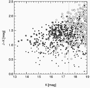
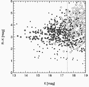
Figure 5: Upper left panel: The distribution of apparent $K$-band magnitudes of galaxies versus redshift in the MUNICS spectroscopic sample. Upper right panel: The $R\!-\!K$-colour versus redshift diagram for galaxies with spectroscopic redshifts. Also shown are model spectral energy distributions from (see text for details), roughly corresponding to Hubble types E (solid line), Sa (dash-dotted line), Sb (dashed line), and Sc (dotted line). Lower left panel: The $J\!-\!K$ versus $K$ colour-magnitude diagram for galaxies (filled circles) and stars (filled triangles) with good-quality spectra. The open circles show the distribution of objects classified as extended in the photometric catalogue of one of the MUNICS fields (S2F1). Also indicated is the magnitude limit of the large and bright spectroscopic sample at $K=17.5$ (dotted line). Lower right panel: Same as lower left panel, but for the distribution of $R\!-\!K$ colours versus apparent $K$-band magnitude.

In the upper panels of the figure, we show distributions of the apparent $K$-band magnitudes and the $R\!-\!K$ colours versus redshift. The comparison of model spectral energy distributions from a combination of empirical spectra and stellar population synthesis models by Maraston (1998) for various Hubble types to the $R\!-\!K$ colours of the objects in the MUNICS spectroscopic catalogue (upper right panel of Fig. 5) shows good agreement, although we seem to miss blue objects at higher redshifts, a fact which must be accounted for in any analysis of this dataset.

The two lower panels of Fig. 5 shows the distribution of extended objects in the photometric catalogue together with the colour distribution of galaxies with spectroscopic redshifts. Comparison shows that the spectroscopic catalogue is a fair representation of the distribution of objects in the photometric sample. Clearly, there is some incompleteness for faint red objects, but this can be corrected for, as will be shown in the following Section.

3.6 Redshift sampling rate and sky coverage

Observations for the spectroscopy of objects from the photometric MUNICS catalogue are almost complete, and most of the fields have been observed with reasonable completeness. The fraction of galaxies with redshift among all galaxies in the photometric catalogue is usually called the redshift sampling rate (e.g. Lin et al. 1999). As an example, Fig. 6 shows the redshift sampling rate of objects in all survey fields with spectroscopic data. The redshift sampling rate is the fraction of objects with successful redshift determination among all galaxies in the photometric catalogue, and, of course, is different from the redshift success rate, which is the fraction of all galaxies with redshift among all galaxies in the spectroscopic catalogue. The redshift success rate depending on apparent magnitude and colours is shown in Fig. 7 and discussed in Section 3.7. These colour distribution should be compared to the distributions of objects from the photometric and spectroscopic catalogue shown in Fig. 5.

Although a few of the masks for the fields still have to be observed, this does not necessarily inhibit the use of the sample for analysis of, e.g., the luminosity function, as long as the sample of objects with successful redshift determination is a fair representation of the total sample, and as long as any systematic incompleteness effects can be corrected for. We will show that this is the case for our catalogue because of the procedure we followed during mask preparation and observation. Firstly, we have tried to select all objects with $K^{\prime}\leq 17.5$ in five survey fields for spectroscopy at Calar Alto. Since the field of view of the spectrograph (MOSCA) is almost as large as the size of our survey field, and since we usually have several masks per magnitude bin (at least for the fainter objects), we are not limited by geometrical constraints from the arrangement of slits on each mask. For the brighter magnitude bins we sometimes had to drop a few objects during the preparation of a mask, but we have tried to include these objects in fainter mask setups. Hence we expect that the small fraction of objects on to which no slit could be put is statistically similar to the distribution of objects to the appropriate magnitude limit. Secondly, all masks which could be observed so far were selected randomly from the masks prepared for observations, so that we do not expect any selection bias here either. Fig. 8 shows the distribution of objects with successful spectroscopy as compared to objects in the photometric catalogue for the survey patches called S2F1, S5F1, S6F5, and S7F5. These particular fields have highest completeness. The field S2F1 contains the sparse sample of fainter objects observed with the VLT. The figure nicely illustrates the statistically homogeneous distribution of the objects in the spectroscopic catalogue. The excess of objects with successful redshift determination visible in the lower half of the field S2F1 is due to foreground structure which can readily be seen in the image itself, showing again the influence of cosmic variance and the importance of having several fields with a relatively large solid angle for the analysis of statistical quantities, one of the huge advantages of the MUNICS project compared to smaller surveys.

Figure 6: The redshift sampling rate, i.e. the fraction of successful redshift determinations among galaxies in the photometric catalogue, as a function of $m_{K}$ (left panel), $R\!-\!K$ (middle panel), and $J\!-\!K$ (right panel) for all galaxies in the survey patches S2F1, S5F1, S6F5, and S7F5 (the field S2F5 has been excluded from further analysis because of the small number of available spectra). The dotted line in the left panel indicates the formal limit of $K\leq 17.5$ of the main part of the spectroscopic survey. The colour distributions in the middle and the right-hand panel are those of objects brighter than this limit.

Figure 7: The redshift success rate, i.e. fraction of successful redshift determinations among all galaxies which were observed spectroscopically, as a function of $m_{K}$ (without any colour constraint; left panel), $R\!-\!K$ (middle panel), and $J\!-\!K$ (right panel) for all galaxies in the survey patches S2F1, S5F1, S6F5, and S7F5). The dotted line in the left panel indicates the formal limit of $K\leq 17.5$ of the main part of the spectroscopic survey. The colour distributions in the middle and the right-hand panel are those of objects brighter than this limit.

3.7 Redshift success rate

The efficiency of redshift determination of spectroscopic observations is described by the redshift success rate rather than the redshift sampling rate. The former is the fraction of objects with secure redshift among all galaxies which were observed spectroscopically and is shown in Fig. 7. As expected, the redshift success rate drops off for very faint and very red objects, but is in general very high due to the good quality of the spectra.

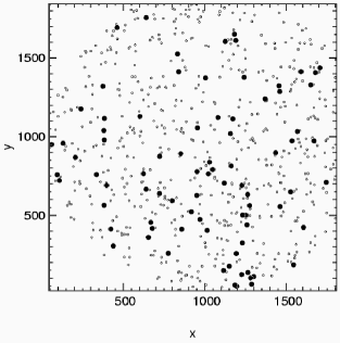
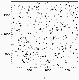
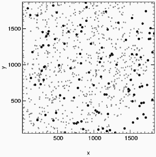
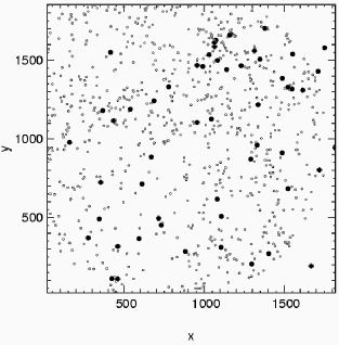
Figure 8: Sky coverage of spectroscopy in the MUNICS fields S2F1 (upper left panel), S5F1 (upper right panel), S6F5 (lower left panel), and S7F5 (lower right panel). The small open circles are objects in the photometric catalogue, the distribution of which is governed by the MUNICS field geometry (see MUNICS I). All galaxies with $K^{\prime}\leq 17.5$ and successful redshift determination are marked by filled circles; they seem to be uniformly distributed on the sky. Note that spectroscopy of the galaxies in the field S7F5 is not complete yet. Coordinates are pixel coordinates in the $K^{\prime}$-band MUNICS frame.

3.8 Extremely red objects

During the last years there has been a lot of research on ‘extremely red objects (EROs)’, usually defined in terms of their very red optical–near-infrared colour ($R\!-\!K>(5\dots 6)$ mag; see, for instance, Martini (2001) and references therein). While the MUNICS catalogue obviously contains such objects, they are not aimed at with the spectroscopic observations described in this paper, mainly because it is very difficult to obtain optical spectra of faint EROs. This is evident from Figures 6 and 7 showing the redshift sampling rate and the redshift success rate for the MUNICS spectroscopic observations. Nevertheless, there are 15 such objects in the spectroscopic catalogue, all having colours of $5.0\;\mathrm{mag}\;\leq R\!-\!K\leq 5.5\;\mathrm{mag}$. Among these we find 7 objects for which no redshift could be determined, 5 galaxies with redshifts $0.46\leq z\leq 1.01$, all having a spectral energy distribution characteristic of early-type galaxies, as well as 3 stars of spectral type M. First results of near-infrared spectroscopy of EROs selected from the MUNICS catalogue are described in Saracco et al. (2003).

4 The near-infrared luminosity function of galaxies

4.1 Calculation of the luminosity function

The luminosity function is computed using the non-parametric $V_{\mathrm{max}}$ formalism (Schmidt, 1968). This method has been shown to yield an unbiased estimate of the luminosity function if the sample is not affected by strong clustering (Takeuchi et al., 2000). Because of our field selection and the relatively large area of the survey, divided into several individual fields, we believe that this assumption is valid for our sample.

The $V_{\mathrm{max}}$ formalism accounts for the fact that some fainter galaxies are not visible in the whole survey volume. Each galaxy $i$ in a given redshift bin $[z_{\mathrm{lower}},z_{\mathrm{upper}}]$ contributes to the number density an amount inversely proportional to the volume $V_{i}$ in which the galaxy is detectable in the survey:

$$V_{i}\;=\;\int\limits_{z_{\mathrm{lower}}}^{\mathrm{min}(z_{\mathrm{upper}},z_{\mathrm{max}})}\>\frac{dV}{dz}\>dz,$$ (1)

where $dV=d\Omega\,r^{2}\,dr$ is the comoving volume element, $d\Omega$ is the solid angle covered by the survey, and $z_{\mathrm{max}}$ is the maximum redshift at which galaxy $i$ having absolute magnitude $M_{i}$ is still detectable given the limiting apparent magnitude of the survey. We have made sure that the effect of the volume correction is of importance only in the faintest bin in absolute magnitude, and that even in this case the correction is small.

Additionally, the contribution of each galaxy $i$ is weighted by the inverse of the detection probability $P(m_{K,i})$ of the $K^{\prime}$-band selected photometric catalogue, where we assume that the detection probability is independent of the galaxy type and can be approximated by that of point-like sources. Completeness simulations for realistic galaxy profiles at various redshifts have shown that this approximation is indeed sufficient for galaxies at redshifts $z<1$ (Snigula et al. 2002, hereafter MUNICS IV). However, since the objects under consideration here are comparatively bright, the influence of this correction is negligible anyway.

In addition to the correction for the incompleteness of the photometric MUNICS catalogue described above, we have to correct for the incompleteness of the spectroscopic catalogue with respect to the photometric sample, described by the redshift sampling rate (see Section 3.6). In principle, this correction depends on the apparent magnitude of the objects (faint objects may produce a lower signal-to-noise ratio or might not have been considered for spectroscopy), on their intrinsic type (it is easier to determine a redshift for objects showing prominent emission lines, for example) and on the redshift of the source (influencing the position of prominent spectral features with respect to the spectral range or bright night-sky emission lines, for example). However, it is difficult to determine a completeness ratio depending on spectral type and redshift, because this information is lacking for all objects without secure redshift measurement.

Hence the redshift sampling rate is often quantified in terms of its dependence on apparent magnitude and two colours instead of spectral type and redshift (see Lin et al. (1999), for example). In this work we compute the redshift sampling rate $C_{i}$,

$$C_{i}\;=\;\frac{N_{z,i}}{N_{i}},$$ (2)

depending on apparent $K^{\prime}$-band magnitude $m_{K}$, and the colours $R\!-\!K$ and $J\!-\!K$. Specifically, for each galaxy $i$ with a redshift, we determine the number $N_{i}$ of galaxies in the photometric sample and the number $N_{z,i}$ of galaxies with successful redshift determination in joint bins of apparent magnitude and colours, where we count all galaxies $j$ obeying

$$\left|m_{K,i}-m_{K,j}\right| \leq 0.70\;\mathrm{mag},$$

$$\left|(R\!-\!K)_{i}-(R\!-\!K)_{j}\right| \leq 0.70\;\mathrm{mag},$$ (3)

$$\left|(J\!-\!K)_{i}-(J\!-\!K)_{j}\right| \leq 0.35\;\mathrm{mag}.$$

On the one hand, the size of the intervals should be large enough to contain a reasonable number of objects to avoid large fluctuations due to small-number statistics. On the other hand, the intervals should not be too large in order to be able to follow the change of the sampling rate. The numbers given in equation (3) have been chosen after careful tests. Note that we have used larger intervals for $m_{K}$ and $R\!-\!K$ since these distributions are broader than the one for $J\!-\!K$. To illustrate the general behaviour of the redshift sampling rate, we show projections of the function in Fig. 6. Note that we have to apply a correction factor of 0.93 to the sampling rate because of stellar contamination of the class of extended objects, a bias introduced by our image-based object classification algorithm, described in detail in Section 2.2.

The near-infrared luminosity function $\Phi(M)$ is then computed according to the formula

$$\Phi(M)\>dM\;=\;\sum\limits_{i}\>\frac{1}{V_{i}}\>\frac{1}{P(m_{K,i})}\>\frac{1}{C_{i}}\>dM,$$ (4)

where the sum runs over all objects $i$ in the redshift range for which we want to calculate the luminosity function.

4.2 Converting to absolute magnitudes

For the conversion of apparent magnitudes $m$ into absolute magnitudes $M$ we need $k(z)$ corrections for the galaxies, defined by

$$M\;=\;m\>-5\,\log\left(\frac{d_{L}(z)}{10\,\mathrm{pc}}\right)\>-2.5\,\log\left(1+z\right)-k(z),$$ (5)

where $d_{L}(z)$ is the cosmological luminosity distance of the galaxy, and $z$ is the redshift.

The $k(z)$ corrections for the objects in the spectroscopic catalogue are obtained by fitting the model spectral energy distributions shown in the left panel of Fig. 9 to the broad-band photometry of the objects. The template spectral energy distributions are constructed by combining empirical spectra and stellar population synthesis models by Maraston (1998). The detailed description of these models will be found in MUNICS II. The $k(z)$ corrections for the $K$ band and the $J$ band are presented in the middle and right panel of Fig. 9, respectively, while Fig. 1 shows a comparison of flux-calibrated spectrum, broad-band photometry, and fitted model spectral energy distribution for two objects in the spectroscopic catalogue.

Figure 9: Left panel: Model spectral energy distributions used to compute $k(z)$ corrections (see text for details). Middle panel: $K$-band $k(z)$ corrections as a function of redshift for the spectral energy distributions shown in the left panel. Right panel: Same as middle panel, but for the $J$ band.

We have also tested the influence of using only one intermediate-type model spectral energy distributions for deriving the $k(z)$ corrections. As is obvious from Fig. 9, this should work well for the $K$ band, where the spread between $k(z)$ corrections for different models is small, but a bit less so well for the $J$ band with its larger variations. Indeed, we do see hardly any difference for the $K$-band luminosity function, and only a small difference in the $J$ band. However, it is important to note that in the following we do not use $k(z)$ corrections from one model, but those from the fitting of template spectral energy distributions to the six-filter broad-band photometry of the MUNICS catalogue.

4.3 The $K$-band luminosity function

The rest-frame $K$-band luminosity function of galaxies drawn from the spectroscopic sample was constructed in the redshift intervals $0.1\leq z\leq 0.3$ (median redshift $z=0.2$), $0.3\leq z\leq 0.6$ (median redshift $z=0.4$, and $0.6\leq z\leq 0.9$ (median redshift $z=0.7$). The two lower redshift bins comprise the majority of objects in the sample, as can be seen in Fig. 3.

The centres of the bins in absolute magnitude were chosen in a way which ensures a fair representation of the bright end of the luminosity function, i.e. the bin centres at the bright end correspond roughly to the absolute magnitudes of the brightest objects in that bin.

Fig. 10 shows the results for the $K$-band luminosity function of galaxies from spectroscopic observations in different redshift bins compared to the luminosity functions determined from the local samples of Loveday (2000) and Kochanek et al. (2001). Clearly there is a good general agreement between the luminosity function measured at $z=0.2$ and the ones from local galaxy samples, although our data seem to suggest a somewhat smaller value for $M_{K}^{*}$. Fitting a Schechter function (Schechter 1976; see also equations (6) and (7) for the parametrisation of the function) to the luminosity function yields the parameters $M_{K}^{*}-5\log h=(-23.79\pm 0.24)$ mag and $\Phi_{K}^{*}=(1.11\pm 0.12)\times 10^{-2}\,h^{3}\,\mathrm{Mpc}^{-3}$. We used a fixed value of $\alpha_{K}=-1.10$, close to the values derived for local galaxies by Loveday (2000) and Kochanek et al. (2001). Contrary to the $J$-band luminosity function discussed below, our normalisation also nicely agrees with the Cole et al. (2001) measurement, although they derive a considerably shallower faint-end slope of $\alpha=-0.93\pm 0.04$. The errors were derived by running Monte-Carlo simulations with 100 000 iterations, taking into account the errors due to the binning in absolute magnitudes. Excluding the faintest magnitude bin does not change the result of the fit significantly.

Note that the agreement between our measurement and the local Schechter functions is also very good at the faint end, although with poor statistics and large correction factors due to the incompleteness. From this we draw the conclusion that our method to correct for incompleteness yields reliable estimates.

At redshifts $0.3\leq z\leq 0.6$, we find a mild evolution of the luminosity function, with a higher characteristic luminosity and a lower normalisation, yielding Schechter parameters of $M_{K}^{*}-5\log h=(-24.04\pm 0.26)$ mag and $\Phi_{K}^{*}=(0.71\pm 0.25)\times 10^{-2}\,h^{3}\,\mathrm{Mpc}^{-3}$. The error contours for the Schechter parameters for the luminosity function in the two lower redshift bins are shown in the same figure. These contours were computed from the $\chi^{2}$ distribution. Finally, we show a comparison of the measurements of the $K$-band luminosity function in all three redshift bins. Although the statistics becomes rather poor in the highest redshift bin with median redshift $z=0.7$, it confirms the trend for the evolution of the luminosity function. However, it is evident that the total evolution out to redshifts around 0.7 is not dramatically large.

Figure 10: The $K$-band luminosity function of galaxies from spectroscopic observations of MUNICS galaxies. Upper left panel: The luminosity function in the redshift range $0.1\leq z\leq 0.3$ (median redshift $z=0.2$; filled symbols). The vertical error bars give the Poissonian error, while the binning error was estimated as $b/\sqrt{12}$ with the size $b$ of the bin. Also shown are the measurements of the local $K$-band luminosity function by Loveday (2000; dotted line) and Kochanek et al. (2001; dashed line), as well as a Schechter approximation to the MUNICS data (solid line). The parameters of the Schechter fit are $M_{K}^{*}-5\log h=(-23.79\pm 0.24)$ mag, $\Phi_{K}^{*}=(1.11\pm 0.12)\times 10^{-2}\,h^{3}\,\mathrm{Mpc}^{-3}$, and $\alpha_{K}=-1.10$ (fixed). Upper right panel: The same as before, but in the redshift range $0.3\leq z\leq 0.6$ (median redshift $z=0.4$), with Schechter parameters $M_{K}^{*}-5\log h=(-24.04\pm 0.26)$ mag, $\Phi_{K}^{*}=(0.71\pm 0.25)\times 10^{-2}\,h^{3}\,\mathrm{Mpc}^{-3}$, and $\alpha_{K}=-1.10$ (fixed). Lower left panel: Error contours ($1\sigma$, $2\sigma$, and $3\sigma$) for the Schechter parameters $M_{K}^{*}$ and $\Phi_{K}^{*}$ from the $\chi^{2}$ distribution. The filled circle indicates the average value of local measurements from Table 12; the “error bars” give an idea of the variation between different authors’ measurements. Lower right panel: The luminosity function in the interval $0.6\leq z\leq 0.9$ (median redshift $z=0.70$; filled circles), compared to the results from the two lower redshift ($z=0.2$, squares; $z=0.4$, triangles) as well as the local measurements.

Comparison of our result with the measurements by Cowie et al. (1996) who derived the $K$-band luminosity function at various redshifts $0<z<1$ from a spectroscopic sample in two small fields shows good agreement with our results. Their values for the Schechter parameters $M_{K}^{*}$, $\Phi_{K}^{*}$, and $\alpha_{K}$ are similar to measurements for local samples. Again, our data favour a slightly larger characteristic luminosity, but the trend of a falling normalisation with redshift is found both in the MUNICS and in the Cowie et al. measurements of the luminosity function.

4.4 The $J$-band luminosity function

The results for the rest-frame $J$-band luminosity function of galaxies from our spectroscopic catalogue are shown in Fig. 11. Note that this is the first determination of the $J$-band luminosity function at higher redshifts following the local measurements by Balogh et al. (2001) and Cole et al. (2001).

Figure 11: The $J$-band luminosity function of galaxies from spectroscopic observations of MUNICS galaxies. Upper left panel: The luminosity function in the redshift range $0.1\leq z\leq 0.3$ (median redshift $z=0.2$; filled symbols). The vertical error bars give the Poissonian error, while the binning error was estimated from $b/\sqrt{12}$ with the size $b$ of the bin. Also shown are the measurement of the local $J$-band luminosity function by Cole et al. (2001) as well as a Schechter approximation to the MUNICS data (solid line). The parameters of the Schechter fit are $M_{J}^{*}-5\log h=(-22.45\pm 0.24)$ mag, $\Phi_{J}^{*}=(1.49\pm 0.22)\times 10^{-2}\,h^{3}\,\mathrm{Mpc}^{-3}$, and $\alpha_{J}=-1.00$ (fixed). Upper right panel: The same as before, but in the redshift range $0.3\leq z\leq 0.6$ (median redshift $z=0.4$), with Schechter parameters $M_{J}^{*}-5\log h=(-23.06\pm 0.24)$ mag, $\Phi_{J}^{*}=(0.76\pm 0.25)\,h^{3}\,\mathrm{Mpc}^{-3}$, and $\alpha_{J}=-1.00$ (fixed). Lower left panel: Error contours ($1\sigma$, $2\sigma$, and $3\sigma$) for the Schechter parameters $M_{J}^{*}$ and $\Phi_{J}^{*}$ in the two lower redshift bins from the $\chi^{2}$ distribution. The filled circle indicates the value of the local measurement by Cole et al. (2001) with the appropriate error bar. Lower right panel: The luminosity function in the interval $0.6\leq z\leq 0.9$ (median redshift $z=0.70$; filled circles) compared to the luminosity function in the two lower redshift bins ($z=0.2$, squares; $z=0.4$, triangles) and the measurements of the local $J$-band luminosity function by Cole et al. (2001).

The Schechter parameters (see equations (6) and (7) for the definition of the Schechter function) derived in the lowest redshift bin ($0.1\leq z\leq 0.3$, median redshift $z=0.2$) are $M_{J}^{*}-5\log h=(-22.45\pm 0.24)$ mag, $\Phi_{J}^{*}=(1.49\pm 0.22)\times 10^{-2}\,h^{3}\,\mathrm{Mpc}^{-3}$ with the faint-end slope $\alpha_{J}$ set to $\alpha_{J}=-1.00$. The errors were derived by running Monte-Carlo simulations with 100 000 iterations, taking into account the errors due to the binning in absolute magnitudes. Compared to the Cole et al. (2001) sample, our measurement seems to favour a similar characteristic magnitude $M_{J}^{*}$, but a somewhat larger value of the normalisation $\Phi_{K}^{*}$. Unfortunately, Balogh et al. (2001), the only other work on the $J$-band luminosity function available so far, do not derive the normalisation, thus the reason for the discrepancy remains unclear. In the $K$-band, the value of the normalisation derived by Cole et al. (2001) is in good agreement with other measurements, although maybe a bit on the low side.

For the intermediate redshift bin $0.3\leq z\leq 0.6$ (median redshift $z=0.4$), the Schechter parameters derived from our data are $M_{J}^{*}-5\log h=(-23.06\pm 0.24)$ mag, $\Phi_{J}^{*}=(0.76\pm 0.25)\,h^{3}\,\mathrm{Mpc}^{-3}$, where $\alpha_{J}$ was again set to a value of $-1.00$. Thus, similar to the $K$-band, we see a mild evolution of the luminosity function with a higher characteristic luminosity and a smaller normalisation. The error contours for the Schechter parameters of the luminosity function in the two lower redshift bins are shown in the same Figure. These contours were derived from the $\chi^{2}$ distribution. At the highest redshifts probed by our sample, the evolution of the $J$-band luminosity function seems to be confirmed, although the statistics becomes rather poor in this case.

Table 8: The uncorrected values $\Phi_{\mathrm{u}}(M_{K})$ of the $K$-band luminosity function, the completeness-corrected values $\Phi(M_{K})$, and their errors $d\Phi(M_{K})$ for the individual redshift intervals and magnitude bins. Here, ‘completeness correction’ refers to the correction of incompleteness of the photometric catalogue, the incompleteness of the spectroscopic sample with respect to the photometric one, and to the $V/V_{\mathrm{max}}$ correction.

$M_{K}-5\log h$	$\Phi_{\mathrm{u}}(M_{K})$	$\Phi(M_{K})$	$d\Phi(M_{K})$
[mag]		[$\mathrm{mag}^{-1}\,h^{3}\,\mathrm{Mpc}^{-3}$]
Median redshift $\langle z\rangle=0.2$:
$-24.825$	$3.25\times 10^{-4}$	$3.89\times 10^{-4}$	$2.75\times 10^{-4}$
$-24.075$	$1.63\times 10^{-3}$	$2.56\times 10^{-3}$	$1.55\times 10^{-3}$
$-23.325$	$5.69\times 10^{-3}$	$6.78\times 10^{-3}$	$2.22\times 10^{-3}$
$-22.575$	$7.64\times 10^{-3}$	$9.68\times 10^{-3}$	$2.88\times 10^{-3}$
$-21.825$	$5.85\times 10^{-3}$	$1.05\times 10^{-2}$	$3.49\times 10^{-3}$
$-21.075$	$3.25\times 10^{-3}$	$1.01\times 10^{-2}$	$4.97\times 10^{-3}$
$-20.325$	$1.14\times 10^{-3}$	$1.75\times 10^{-2}$	$1.22\times 10^{-2}$
Median redshift $\langle z\rangle=0.4$:
$-25.625$	$2.93\times 10^{-5}$	$3.90\times 10^{-5}$	$3.90\times 10^{-5}$
$-24.875$	$4.69\times 10^{-4}$	$6.91\times 10^{-4}$	$3.42\times 10^{-4}$
$-24.125$	$1.41\times 10^{-3}$	$2.44\times 10^{-3}$	$7.14\times 10^{-4}$
$-23.375$	$1.50\times 10^{-3}$	$4.12\times 10^{-3}$	$1.32\times 10^{-3}$
$-22.625$	$8.51\times 10^{-4}$	$3.86\times 10^{-3}$	$1.27\times 10^{-3}$
Median redshift $\langle z\rangle=0.7$:
$-25.825$	$1.50\times 10^{-5}$	$1.87\times 10^{-5}$	$1.87\times 10^{-5}$
$-25.075$	$1.65\times 10^{-4}$	$4.20\times 10^{-4}$	$2.37\times 10^{-4}$
$-24.325$	$2.84\times 10^{-4}$	$1.14\times 10^{-3}$	$4.42\times 10^{-4}$
$-23.575$	$1.35\times 10^{-4}$	$9.63\times 10^{-4}$	$4.59\times 10^{-4}$

Table 9: The uncorrected values $\Phi_{\mathrm{u}}(M_{J})$ of the $J$-band luminosity function, the completeness-corrected values $\Phi(M_{J})$, and their errors $d\Phi(M_{J})$ for the individual redshift intervals and magnitude bins. Here, ‘completeness correction’ refers to the correction of incompleteness of the photometric catalogue, the incompleteness of the spectroscopic sample with respect to the photometric one, and to the $V/V_{\mathrm{max}}$ correction.

$M_{J}-5\log h$	$\Phi_{\mathrm{u}}(M_{J})$	$\Phi(M_{J})$	$d\Phi(M_{J})$
[mag]		[$\mathrm{mag}^{-1}\,h^{3}\,\mathrm{Mpc}^{-3}$]
Median redshift $\langle z\rangle=0.2$:
$-23.775$	$1.63\times 10^{-4}$	$1.63\times 10^{-4}$	$1.63\times 10^{-4}$
$-23.025$	$1.95\times 10^{-3}$	$2.88\times 10^{-3}$	$1.70\times 10^{-3}$
$-22.275$	$6.34\times 10^{-3}$	$7.55\times 10^{-3}$	$2.30\times 10^{-3}$
$-21.525$	$6.50\times 10^{-3}$	$8.26\times 10^{-3}$	$2.68\times 10^{-3}$
$-20.775$	$6.50\times 10^{-3}$	$1.13\times 10^{-2}$	$3.55\times 10^{-3}$
Median redshift $\langle z\rangle=0.4$:
$-24.725$	$2.93\times 10^{-5}$	$3.90\times 10^{-5}$	$3.90\times 10^{-5}$
$-23.975$	$4.40\times 10^{-4}$	$6.58\times 10^{-4}$	$3.21\times 10^{-4}$
$-23.225$	$1.20\times 10^{-3}$	$2.37\times 10^{-3}$	$7.57\times 10^{-4}$
$-22.475$	$1.61\times 10^{-3}$	$3.94\times 10^{-3}$	$1.16\times 10^{-3}$
$-21.725$	$9.68\times 10^{-4}$	$4.02\times 10^{-3}$	$1.24\times 10^{-3}$
Median redshift $\langle z\rangle=0.7$:
$-24.675$	$2.99\times 10^{-5}$	$3.67\times 10^{-5}$	$3.67\times 10^{-5}$
$-23.925$	$2.84\times 10^{-4}$	$8.41\times 10^{-4}$	$3.89\times 10^{-4}$
$-23.175$	$2.24\times 10^{-4}$	$9.72\times 10^{-4}$	$4.21\times 10^{-4}$

5 Discussion

To quantify the redshift evolution of the near-infrared luminosity functions, we performed both Kolmogorov-Smirnov tests for the cumulative distributions of absolute magnitudes and a $\chi^{2}$ analysis for the redshift evolution of the Schechter parameters.

5.1 Kolmogorov-Smirnov tests

One method to compare the measurements of the near-infrared luminosity functions at various redshifts is to apply the Kolmogorov-Smirnov test to the cumulative distribution of objects in absolute magnitudes. Of course, completeness and $1/V_{\mathrm{max}}$ corrections have to be applied to each individual object entering the distribution. The advantage of this method is that it uses the absolute magnitudes as measured in the sample without binning. Furthermore, it is independent of the relative normalisation of the samples one wants to compare.

We firstly have run this test by comparing the cumulative luminosity distributions from our data in the three redshift bins to the local measurements of the luminosity function. The results are shown in Table 10 for the $K$-band, and Table 11 for the $J$-band, respectively. Furthermore, we show the resulting cumulative distributions in Figures 12 and 13 for the $K$ band and the $J$ band, respectively.

While the cumulative distributions are in fair agreement for the lower redshift bin ($0.1<z<0.3$), they are significantly different for the two higher redshift bins ($0.3<z<0.6$ and $0.6<z<0.9$, respectively), confirming the result found from the fitting of Schechter parameters $M^{*}$ and $\Phi^{*}$.

Table 10: Probabilities for compatible cumulative distributions of absolute magnitudes derived from a Kolmogorov-Smirnov test. The comparison distributions are derived from the local luminosity function measurements by Loveday (2000) and Kochanek et al. (2001). The magnitudes in the second column are upper limits to the range of absolute magnitudes for which the distribution has been computed.

Redshift	$M_{K}$ [mag]	Loveday (2000)	Kochanek et al. (2001)
$\langle z\rangle=0.2$	$-21.5$	35.73 %	26.10 %
$\langle z\rangle=0.4$	$-23.0$	0.88 %	0.15 %
$\langle z\rangle=0.7$	$-24.0$	1.61 %	0.37 %

Table 11: Probabilities for compatible cumulative distributions of absolute magnitudes derived from a Kolmogorov-Smirnov test. The comparison distribution is derived from the local luminosity function measurement by Cole et al. (2001). The magnitudes in the second column are upper limits to the range of absolute magnitudes for which the distribution has been computed.

Redshift	$M_{J}$ [mag]	Cole et al. (2001)
$\langle z\rangle=0.2$	$-20.3$	21.51 %
$\langle z\rangle=0.4$	$-21.6$	0.01 %
$\langle z\rangle=0.7$	$-22.9$	0.07 %

Figure 12: Resulting cumulative distribution functions for the absolute $K$-band magnitudes from the MUNICS spectroscopic catalogue (solid line) as compared to the local measurements by Loveday (2000; dotted line) and Kochanek et al. (2001; dashed line). The diagram on the left-hand side compares the $0.1<z<0.3$ redshift bin to the local one, the middle diagram shows the same for the $0.3<z<0.6$ redshift interval, and the diagram on the right-hand side compares the distributions in the $0.6<z<0.9$ interval to the local ones. The values quoted in the diagrams give the probabilities that both cumulative distributions are drawn from the same population.

Figure 13: Resulting cumulative distribution functions for the absolute $J$-band magnitudes from the MUNICS spectroscopic catalogue (solid line) as compared to the local measurements by Cole et al. (2001; dashed line). The diagram on the left-hand side compares the $0.1<z<0.3$ redshift bin to the local one, the middle diagram shows the same for the $0.3<z<0.6$ redshift interval, and the diagram on the right-hand side compares the distribution in the $0.6<z<0.9$ interval to the local one. The values quoted in the plots give the probabilities that both cumulative distributions are drawn from the same population.

As an additional test we have applied the Kolmogorov-Smirnov test to the cumulative distributions from the two lower redshift bins. The results of this test are shown in Fig. 14, where one can see that the probabilities that both distributions are drawn from the same parent population are very small.

Figure 14: Cumulative distributions in absolute magnitude for the two lower redshift bins and results from a Kolmogorov-Smirnov test applied to these data, both for the $K$ band (left panel) and the $J$ band (right panel).

5.2 Likelihood analysis of luminosity function evolution

In this Section we will describe a $\chi^{2}$ analysis of the redshift evolution of the near-infrared luminosity functions. This test uses the Schechter parametrisation

$$\Psi\,(L)\;=\;\frac{\Phi^{*}}{L^{*}}\,\left(\frac{L}{L^{*}}\right)^{\alpha}\,\exp\left(-\frac{L}{L^{*}}\right)$$ (6)

of the luminosity function, where $L^{*}$ is the characteristic luminosity, $\alpha$ the faint-end slope, and $\Phi^{*}$ the normalisation of the luminosity function (Schechter, 1976). The corresponding equation in absolute magnitudes reads

$$\Psi\,(M) = \frac{2}{5}\,\Phi^{*}\,\ln 10\>10^{0.4(M^{*}-M)(1+\alpha)}$$ (7)

$$\exp\left(-10^{0.4(M^{*}-M)}\right).$$

To estimate the rate of evolution of the parameters with redshift, we define evolution parameters $\mu$ and $\nu$ as follows:

$$\Phi^{*}\,(z) = \Phi^{*}\,(0)\>\left(1\,+\,\mu z\right),$$

$$M^{*}\,(z) = M^{*}\,(0)\,+\,\nu z,\;\mathrm{and}$$ (8)

$$\alpha\,(z) = \alpha\,(0)\;\;\equiv\;\;\alpha.$$

Note that the faint end of the luminosity function cannot be determined very well from our data, thus we leave the faint-end slope $\alpha$ of the Schechter luminosity function fixed, as we have also done during the fitting of a Schechter function to our data.

To quantify the redshift evolution of $\Phi^{*}$ and $M^{*}$ we now compare our luminosity function data in all redshift bins with the local Schechter function evolved according to equation (8) to the appropriate redshift. We do this for a grid of values for $\mu$ and $\nu$, and calculate the value of $\chi^{2}$ for each grid point according to

$$\chi^{2}\,(\mu,\nu)\;=\;\frac{1}{n}\,\sum_{i=1}^{N}\,\frac{\left[\Phi(M_{i},z_{i})-\Psi(M_{i},\mu,\nu,z_{i})\right]^{2}}{\sigma_{i}^{2}},$$ (9)

where $\Phi(M,z)$ is the measurement of the luminosity function at median redshift $z$ in the magnitude bin centred on $M$, $\Psi(M,\mu,\nu,z)$ is the local Schechter function evolved according to the evolution model defined in equation (8) to the redshift $z$, $\sigma_{i}$ is the RMS error of the luminosity function value, and $n$ is the number of free parameters of the approximation, i.e. the number of data points used minus the number of parameters derived from the fitting.

We want to compare our measurement of the $K$-band luminosity function with the Schechter approximations to the local determinations. We use the measurements by Loveday (2000) and Kochanek et al. (2001) for the $K$-band (since the luminosity function parameters derived from local samples are very similar anyway), and the local $J$-band luminosity function is the one by Cole et al. (2001). The Schechter parameters derived by those authors are shown in Tables 12 and 13. Chosing a shallower faint-end slope in the $K$ band, similar to the one derived by Cole et al. (2001), changes the result slightly, but – within the errors – not significantly.

To avoid that data points with large completeness correction factors affect the result, we exclude all luminosity function measurements with a total correction factor (photometric incompleteness, spectroscopic incompleteness, and $V/V_{\mathrm{max}}$ correction) larger than three.

The result of the likelihood analysis is shown in Fig. 15. For the $K$-band, we compare our measurements at redshifts $0.2$, $0.4$, and $0.7$ to the local measurements by Loveday (2000) and Kochanek et al. (2001), and to the average of their Schechter parameters. We detect a brightening of $\Delta M_{K}^{*}/\Delta z\simeq 0.70$ magnitudes, and a decline of the number density of objects to redshift one. The decrease of $\Phi_{K}^{*}$ with redshift is obviously quite strongly dependent on the parameters of the local luminosity function, however, for the average value we derive $\Delta\Phi_{K}^{*}/(\Phi_{K}^{*}\Delta z)\simeq-0.35$. These results also give quantitative estimates of the evolution which can already be seen in the Schechter parameters derived from our data, see Table 8 for details. Note that Huang et al. (2002) derive a significantly brighter $M^{*}$, a slightly larger normalisation, and a steeper faint-end slope, which they ascribe to redshift selection effects. If their measurements are valid, the brightening to redshift one would be smaller, whereas the evolution in number density would be even larger.

Within the errors, the results found in this work agree nicely with the measurements of the $K$-band luminosity function derived from the full MUNICS sample based on photometric redshifts. First results are shown in MUNICS III and show the same trend for the evolution of the luminosity function with redshift. A more detailed analysis will be shown in MUNICS II, where the evolutionary trend with a brightening of 0.5 to 0.7 mag and a decrease in number density of roughly 25 per cent to redshift one is confirmed.

In the case of the $J$-band (right panel of Fig. 15), the evolution of the luminosity function is obviously not constrained. This is also apparent from the error contours of the Schechter parameters shown in Fig. 11 (lower left panel), where one can see that the local measurement by Cole et al. (2001) has a characteristic magnitude similar to the one derived in our lowest redshift bin, but a normalisation in between the ones derived from our two lower redshift intervals, thus making any conclusions about evolution with respect to the local sample difficult. Nevertheless, we note that our $J$-band luminosity function data seem to confirm the trend seen for the $K$ band, which is also evident from the Kolmogorov-Smirnov tests presented in Section 5.1.

Figure 15: Left panel: Result of the estimation of the redshift evolution of the Schechter parameters $M_{K}^{*}$ and $\Phi_{K}^{*}$ between $z=0.4$ (MUNICS luminosity function) and the local universe from Loveday (2000; dotted line), Kochanek et al. (2001; dashed line), and for an average of these two local measurements (solid line) as derived from a $\chi^{2}$ approach (see text for details). The contours correspond to $1\sigma$, $2\sigma$, and $3\sigma$ confidence level. The $d\Phi^{*}/dz=0$ and $dM^{*}/dz=0$ lines indicate the non-evolution values. Right panel: The same for the $J$-band luminosity function. In this case, the local measurement is taken from Cole et al. (2001, dotted line), with the appropriate Schechter parameters from Table 13, and the evolution is very badly constrained.

Table 12: Summary of samples used for deriving the $K$-band field-galaxy luminosity function, giving the source for the data, the approximate limiting magnitude (either in the optical or in the near-infrared), the approximate area, the number of objects, the redshift range of the survey (either as interval or as median redshift) and the parameters of the Schechter function derived from the data. Parameters without error estimate were kept fixed during the fitting procedure. Where necessary, the values quoted have been converted from the cosmology originally used to the $\Omega_{m}=0.3$, $\Omega_{\Lambda}=0.7$ cosmology following Cole et al. (2001).

Source	Limit	Area	#	$z$	$M_{K}^{*}-5\log h$	$\alpha_{K}$	$\Phi_{K}^{*}$
	[mag]	[arcmin2]			[mag]		[$10^{-2}h^{3}\mathrm{Mpc}^{-3}$]
Mobasher et al. (1993)	$B_{J}\leq 17$, $K\leq$13.0		181	0.0…0.1	$-$23.37 $\pm$ 0.30	$-$1.00 $\pm$ 0.30	1.12 $\pm$ 0.16
Songaila et al. (1994)	$K\leq$14.5…20.0	5544…5
Glazebrook et al. (1995)	$K\leq$17.0	552	124	0.0…0.8	$-$23.14 $\pm$ 0.23	$-$1.04	2.22 $\pm$ 0.53
Cowie et al. (1996)	$K\leq$19.5	26	254	0.2…1.0	$-$23.49 $\pm$ 0.10	$-$1.25 $\pm$ 0.15	0.80 $\pm$ 0.20
Gardner et al. (1997)	$K\leq$15.0	15840	567	0.14	$-$23.30 $\pm$ 0.17	$-$1.00 $\pm$ 0.24	1.44 $\pm$ 0.20
Szokoly et al. (1998)	$R_{F}\leq 18.5$, $K\leq$16.5	2160	175	0.0…0.4	$-$23.80 $\pm$ 0.30	$-$1.30 $\pm$ 0.20	0.86 $\pm$ 0.29
Loveday (2000)	$K\leq$12.0		363	0.05	$-$23.58 $\pm$ 0.42	$-$1.16 $\pm$ 0.19	1.20 $\pm$ 0.08
Kochanek et al. (2001)	$K_{20}\leq 11.25$		4192	0.02	$-$23.43 $\pm$ 0.05	$-$1.09 $\pm$ 0.06	1.16 $\pm$ 0.10
Cole et al. (2001)	$b_{J}\leq 19.5$, $K\leq 13$	2.2 106	17173	0.05	$-$23.36 $\pm$ 0.02	$-$0.93 $\pm$ 0.04	1.16 $\pm$ 0.17
Balogh et al. (2001)	$R_{c}\leq 15\dots 17$, $K\leq 13$			0.0…0.18	$-$23.48 $\pm$ 0.08	$-$1.10 $\pm$ 0.14
Huang et al. (2002)	$K\leq 15$		1065	0.138	$-$23.70 $\pm$ 0.08	$-$1.39 $\pm$ 0.09	1.30 $\pm$ 0.20
MUNICS (this work)	$K\leq 17.5\dots 19.0$	649	157	0.1…0.3	$-$23.79 $\pm$ 0.24	$-$1.10	1.11 $\pm$ 0.12
			145	0.3…0.6	$-$24.04 $\pm$ 0.26	$-$1.10	0.71 $\pm$ 0.25

Table 13: Summary of samples used for deriving the $J$-band field-galaxy luminosity function, giving the source for the data, the approximate limiting magnitude (either in the optical or in the near-infrared), the approximate area, the number of objects, the redshift range of the survey (either as interval or as median redshift), and the parameters of the Schechter function derived from the data. Parameters without error estimate were kept fixed during the fitting procedure.

Source	Limit	Area	#	$z$	$M_{J}^{*}-5\log h$	$\alpha_{J}$	$\Phi_{J}^{*}$
	[mag]	[arcmin2]			[mag]		[$10^{-2}h^{3}\mathrm{Mpc}^{-3}$]
Cole et al. (2001)	$b_{J}\leq 19.5$, $K\leq 13$	2.2 106	17173	0.05	$-$22.36 $\pm$ 0.02	$-$0.93 $\pm$ 0.04	1.08 $\pm$ 0.16
Balogh et al. (2001)	$R_{c}\leq 15\dots 17$, $K\leq 13$			0.0…0.18	$-$22.23 $\pm$ 0.07	$-$0.96 $\pm$ 0.12
MUNICS (this work)	$K\leq 17.5\dots 19.0$	649	132	0.1…0.3	$-$22.45 $\pm$ 0.24	$-$1.00	1.49 $\pm$ 0.22
			145	0.3…0.6	$-$23.06 $\pm$ 0.24	$-$1.00	0.76 $\pm$ 0.25

6 Conclusions

We have presented spectroscopic follow-up observations of galaxies from the Munich Near-Infrared Cluster Survey (MUNICS), described the observations, the data-reduction and the properties of the spectroscopic sample. Furthermore we have presented the rest-frame $K$-band luminosity function for galaxies at median redshifts of $z=0.2$, $z=0.4$, and $z=0.7$. The Schechter parameters derived at redshift $z=0.2$ are $M_{K}^{*}-5\log h=(-23.79\pm 0.24)$ mag, $\Phi_{K}^{*}=(1.11\pm 0.12)\times 10^{-2}\,h^{3}\,\mathrm{Mpc}^{-3}$ for fixed $\alpha_{K}=-1.10$ as measured locally, in good agreement to values derived at low redshifts. At redshift $z=0.4$, however, the Schechter parameters are $M_{K}^{*}-5\log h=(-24.04\pm 0.26)$ mag and $\Phi_{K}^{*}=(0.71\pm 0.25)\times 10^{-2}\,h^{3}\,\mathrm{Mpc}^{-3}$ (for the same value of $\alpha_{K}$). Thus the value for the characteristic luminosity is somewhat larger and the normalisation smaller than the ones derived locally. This is confirmed by Kolmogorov-Smirnov tests for the cumulative distributions in absolute magnitudes, and by a $\chi^{2}$ analysis for the evolution of the luminosity function. From the latter we find mild evolution in magnitudes ($\Delta M_{K}^{*}=-0.70\pm 0.30$ mag) and number densities ($\Delta\Phi_{K}^{*}/\Phi_{K}^{*}=-0.35\pm 0.30$) to redshift one. Furthermore, we have presented the first measurement of the $J$-band luminosity function of galaxies at higher redshifts with Schechter parameters $M_{J}^{*}-5\log h=(-22.45\pm 0.24)$ mag, $\Phi_{J}^{*}=(1.49\pm 0.22)\times 10^{-2}\,h^{3}\,\mathrm{Mpc}^{-3}$ for $z=0.2$, and $M_{J}^{*}-5\log h=(-23.06\pm 0.24)$ mag, $\Phi_{J}^{*}=(0.76\pm 0.25)\,h^{3}\,\mathrm{Mpc}^{-3}$ for $z=0.4$, showing the same trend of evolution as the $K$-band luminosity function. The faint-end slope $\alpha_{J}$ set to a value of $-1.00$ in both redshift bins. The evolutionary trend of the near-infrared luminosity of $K$-selected galaxies described above is consistent with expectations from pure luminosity evolution, while the decrease in number density with redshift can be understood in the context of hierarchical galaxy formation models.

References

- Balogh et al. (2001) Balogh M. L., Christlein D., Zabludoff A. I., Zaritsky D., 2001, ApJ, 557, 117
- Brinchmann & Ellis (2000) Brinchmann J., Ellis R. S., 2000, ApJ, 536, L77
- Cole et al. (2001) Cole S., et al., 2001, MNRAS, 326, 255
- Cowie et al. (1996) Cowie L. L., Songaila A., Hu E. M., Cohen J. G., 1996, AJ, 112, 839
- Drory et al. (2003) Drory N., Bender R., Feulner G., Hopp U., Snigula J., Maraston C., Hill G., 2003, in preparation (MUNICS II)
- Drory et al. (001b) Drory N., Bender R., Snigula J., Feulner G., Hopp U., Maraston C., Hill G. J., Mendes de Oliveira C., 2001b, ApJ, 562, L111 (MUNICS III)
- Drory et al. (001a) Drory N., Feulner G., Bender R., Botzler C. S., Hopp U., Maraston C., Mendes de Oliveira C., Snigula J., 2001a, MNRAS, 325, 550 (MUNICS I)
- Ellis (1997) Ellis R. S., 1997, ARA&A, 35, 389
- Falco et al. (1999) Falco E. E., Kurtz M. J., Geller M. J., Huchra J. P., Peters J., Berlind P., Mink D. J., Tokarz S. P., Elwell B., 1999, PASP, 111, 438
- Folkes et al. (1999) Folkes S., et al., 1999, MNRAS, 308, 459
- Gössl & Riffeser (2002) Gössl C. A., Riffeser A., 2002, A&A, 381, 1095
- Gardner et al. (1997) Gardner J. P., Sharples R. M., Frenk C. S., Carrasco B. E., 1997, ApJ, 480, L99
- Geller & Huchra (1989) Geller M. J., Huchra J. P., 1989, Science, 246, 897
- Glazebrook et al. (1995) Glazebrook K., Peacock J. A., Miller L., Collins C. A., 1995, MNRAS, 275, 169
- Hill et al. (1998) Hill G. J., Nicklas H. E., MacQueen P. J., Tejada C., Cobos Duenas F. J., Mitsch W., 1998, in Sandro D’Odorico ed., Proc. SPIE, Optical Astronomical Instrumentation Vol. 3355. p. 375
- Hopp & Fernández (2002) Hopp U., Fernández M., 2002, Calar Alto Newsletter, 4, available at http://www.caha.es/newsletter/news02a/hopp/paper.pdf
- Huang et al. (2002) Huang J.-S., Glazebrook K., Cowie L. L., Tinney C., 2002, astro-ph/0209440
- Jarrett et al. (2000) Jarrett T. H., Chester T., Cutri R., Schneider S., Skrutskie M., Huchra J. P., 2000, AJ, 119, 2498
- Kauffmann & Charlot (1998) Kauffmann G., Charlot S., 1998, MNRAS, 297, L23
- Kochanek et al. (2001) Kochanek C. S., Pahre M. A., Falco E. E., Huchra J. P., Mader J., Jarrett T. H., Chester T., Cutri R., Schneider S. E., 2001, ApJ, 560, 566
- Lin et al. (1999) Lin H., Yee H. K. C., Carlberg R. G., Morris S. L., Sawicki M., Patton D. R., Wirth G., Shepherd C. W., 1999, ApJ, 518, 533
- Loveday (2000) Loveday J., 2000, MNRAS, 312, 557
- Loveday et al. (1996) Loveday J., Peterson B. A., Maddox S. J., Efstathiou G., 1996, ApJS, 107, 201
- Maddox et al. (1990) Maddox S. J., Efstathiou G., Sutherland W. J., Loveday J., 1990, MNRAS, 243, 692
- Maraston (1998) Maraston C., 1998, MNRAS, 300, 872
- Martini (2001) Martini P., 2001, AJ, 121, 2301
- Mobasher et al. (1993) Mobasher B., Sharples R. M., Ellis R. S., 1993, MNRAS, 263, 560
- Munn et al. (1997) Munn J. A., Koo D. C., Kron R. G., Majewski S. R., Bershady M. A., Smetanka J. J., 1997, ApJS, 109, 45
- Osterbrock et al. (1997) Osterbrock D. E., Fulbright J. P., Bida T. A., 1997, PASP, 109, 614
- Osterbrock et al. (1996) Osterbrock D. E., Fulbright J. P., Martel A. R., Keane M. J., Trager S. C., Basri G., 1996, PASP, 108, 277
- Peterson et al. (1986) Peterson B. A., Ellis R. S., Efstathiou G., Shanks T., Bean A. J., Fong R., Zen-Long Z., 1986, MNRAS, 221, 233
- Rix & Rieke (1993) Rix H., Rieke M. J., 1993, ApJ, 418, 123
- Saracco et al. (2003) Saracco P., Longhetti M., Severgnini P., Della Ceca R., Mannucci F., Bender R., Drory N., Feulner G., Ghinassi F., Hopp U., Maraston C., 2003, A&A, 398, 127
- Schechter (1976) Schechter P., 1976, ApJ, 203, 297
- Schmidt (1968) Schmidt M., 1968, ApJ, 151, 393
- Seifert et al. (1994) Seifert W., Mitsch W., Nicklas H., Rupprecht G., 1994, in David L. Crawford, Eric R. Craine ed., Proc. SPIE, Instrumentation in Astronomy VIII Vol. 2198. p. 213
- Shectman et al. (1996) Shectman S. A., Landy S. D., Oemler A., Tucker D. L., Lin H., Kirshner R. P., Schechter P. L., 1996, ApJ, 470, 172
- Snigula et al. (2002) Snigula J., Drory N., Bender R., Botzler C. S., Feulner G., Hopp U., 2002, MNRAS, 336, 1329 (MUNICS IV)
- Songaila et al. (1994) Songaila A., Cowie L. L., Hu E. M., Gardner J. P., 1994, ApJS, 94, 461
- Szokoly et al. (1998) Szokoly G. P., Subbarao M. U., Connolly A. J., Mobasher B., 1998, ApJ, 492, 452
- Takeuchi et al. (2000) Takeuchi T. T., Yoshikawa K., Ishii T. T., 2000, ApJS, 129, 1