Optical and radio behaviour of the BL Lacertae object 0716+714

see next page

Abstract. Eight optical and four radio observatories have been intensively monitoring the BL Lac object 0716+714 in the last years: 4854 data points have been collected in the $UBVRI$ bands since 1994, while radio light curves extend back to 1978. Many of these data, which all together constitute the widest optical and radio database available on this object, are presented here for the first time. Four major optical outbursts were observed at the beginning of 1995, in late 1997, at the end of 2000, and in fall 2001. In particular, an exceptional brightening of 2.3 mag in 9 days was detected in the $R$ band just before the BeppoSAX pointing of October 30, 2000. A big radio outburst lasted from early 1998 to the end of 1999. The long-term trend shown by the optical light curves seems to vary with a characteristic time scale of about 3.3 years, while a longer period of 5.5–6 years seems to characterize the radio long-term variations. In general, optical colour indices are only weakly correlated with brightness; a clear spectral steepening trend was observed during at least one long-lasting dimming phase. Moreover, the optical spectrum became steeper after $\rm JD\sim 2451000$, the change occurring in the decaying phase of the late-1997 outburst. The radio flux behaviour at different frequencies is similar, but the flux variation amplitude decreases with increasing wavelength. The radio spectral index varies with brightness (harder when brighter), but the radio fluxes seem to be the sum of two different-spectrum contributions: a steady base level and a harder-spectrum variable component. Once the base level is removed, the radio variations appear as essentially achromatic, similarly to the optical behaviour. Flux variations at the higher radio frequencies lead the lower-frequency ones with week–month time scales. The behaviour of the optical and radio light curves is quite different, the broad radio outbursts not corresponding in time to the faster optical ones and the cross-correlation analysis indicating only weak correlation with long time lags. However, minor radio flux enhancements simultaneous with the major optical flares can be recognized, which may imply that the mechanism producing the strong flux increases in the optical band also marginally affects the radio one. On the contrary, the process responsible for the big radio outbursts does not seem to affect the optical emission.

1 Introduction

Understanding blazar variability is one of the major issues of active galactic nuclei (AGNs) studies. Blazars, i.e. BL Lac objects and flat-spectrum radio quasars, are known to be very active across all the electromagnetic spectrum, exhibiting flux variations on different time scales, from years down to hours or less. It is widely accepted that the variations recognizable in the blazar light curves are due to the superposition of a number of components: in general, one can say that a long-term trend, maybe achromatic (e.g. Ghisellini et al. ghi97 (1997); Villata et al. vil02 (2002)), possibly periodic (e.g. Smith & Nair smi95 (1995); Raiteri et al. rai01 (2001)), determines the base-level flux oscillations. Faster variations, often implying spectral changes (e.g. Ghisellini et al. ghi97 (1997); Villata et al. vil00 (2000), vil02 (2002)), are likely caused by a different physical mechanism.

Verifying the existence of correlations among the flux variations in different bands is of uttermost importance in order to shed light on the processes which are at the origin of the variations themselves. In particular, it is important to investigate whether a correlation exists between the optical and radio emissions, which are both ascribed to synchrotron radiation from relativistic electrons in a plasma jet.

Many studies have been devoted to this main point, but the results for different sources do not show a common behaviour. On short time scales, intraday variability (IDV) in radio and optical bands sometimes appeared to be likely correlated (see Quirrenbach et al. qui91 (1991) and Wagner et al. wag96 (1996) for 0716+714; Kraus et al. kra99 (1999) for 0235+164). On longer time scales, when correlations are found, there may be delays among variations in different bands, changes at the higher frequencies usually leading those at the lower ones (Tornikoski et al. tor94 (1994); Clements et al. cle95 (1995); Raiteri et al. rai01 (2001)).

In this paper we present the most complete optical and radio light curves of S5 0716+71 available up to now. Most of the $BVRI$ observations were carried out starting from 1994 by the blazar monitoring groups of the Perugia and Roma Universities and of the Torino Observatory, as part of a long-standing collaboration aiming at studying this BL Lac object. Previous, partial results obtained by the collaboration have already been published: an analysis of the data of the first season can be found in Ghisellini et al. (ghi97 (1997)), while an update of the $R$ light curve up to April 1998 was presented by Massaro et al. (mas99 (1999)). Data taken during the coordinated BeppoSAX and optical observations of November 14, 1996 and November 7, 1998 were reported by Giommi et al. (gio99 (1999)). Finally, the results of observations performed during the Whole Earth Blazar Telescope (WEBT; http://www.to.astro/blazars/webt/) campaign of February 1999 appeared in Villata et al. (vil00 (2000)). Other optical data have been taken at the Abastumani Observatory since 1997. The Mount Maidanak Observatory joined the collaboration during winter 2000–2001, while optical data simultaneous with the X-ray data taken by the BeppoSAX satellite on October 30, 2000 were provided by the Skinakas Observatory.

The source 0716+714 is one of the targets of the radio monitoring programs at the Metsähovi Radio Observatory (Teräsranta et al. ter98 (1998)), at the University of Michigan Radio Astronomy Observatory (UMRAO; Aller et al. all85 (1985), all99 (1999)), and at the Max-Planck-Institut für Radioastronomie in Bonn (Peng et al. pen00 (2000)). It is also observed in the millimetric band at the Instituto de Radioastronomia Millimetrica in Granada (IRAM; Steppe et al. ste88 (1988), ste92 (1992), ste93 (1993); Reuter et al. reu97 (1997)).

A preliminary study of the cross-correlation between the Metsähovi plus UMRAO radio data and the optical ones was presented by Raiteri et al. (rai99 (1999)).

The paper is organized as follows: in Sect. 2 we review previous studies on S5 0716+71 in the optical and radio bands. Optical and radio observation techniques are described in Sect. 3, while light curves are presented in Sects. 4 and 5. Timing analysis and correlations among bands are discussed in Sect. 6. The conclusions are drawn in Sect. 7.

2 S5 0716+71

The BL Lacertae object 0716+714 was included in the S5 catalog of the Strong Source Survey performed at 4.9 GHz (Kühr et al. kuh81 (1981)). Radio maps reveal a compact core-jet structure and an extended emission resembling an FR II object (Antonucci et al. ant86 (1986); Gabuzda et al. gab98 (1998)). Old estimates of apparent velocity raised the issue of the existence of superluminal motion in this source (Gabuzda et al. gab98 (1998)); however, a recent determination of proper motions by Jorstad et al. (jor01 (2001)) resulted in values greater than 11–$15\,h^{-1}\,c$. These latter authors also found that the ejection of VLBA components may be quasi-periodic, occurring every $\sim 0.7\,\rm yr$. The ongoing multifrequency VLBI monitoring (1992–2002; Bach et al. bac02 (2002)) by the Bonn group is consistent with the fast-motion scenario suggested by Jorstad et al. (jor01 (2001)). The combination of now more than 26 VLBI observations at 5–22 GHz results in apparent velocities of 5–$10\,h^{-1}\,c$, with different components moving at slightly different speeds. A full analysis of the detailed source kinematics will be given by Bach et al. (bac03 (2003)).

VLA and VLBI observations at 6 cm show rapid polarization variability, which is probably produced in some compact feature at about 25 mas from the nucleus (Gabuzda et al. gab00 (2000)). Polarization in the optical band was found to be variable on short time scales too, with possible periods of 12.5, 2.5, and 0.14 days (Impey et al. imp00 (2000)).

Spectroscopic observations of S5 0716+71 have failed to reveal any feature up to now (Stickel et al. sti93 (1993); Rector & Stocke rec01 (2001)), so that the redshift of this source is still undetermined. However, a number of observational considerations as the starlike appearance (Stickel et al. sti93 (1993)), the absence of a host galaxy, and the small angular size of the extended halo in radio maps (Wagner et al. wag96 (1996)) suggest $z>0.3$.

Not many photometric data are available in the literature for 0716+714 before our starting observing date. Biermann et al. (bie81 (1981)) reported variability in magnitude, polarization, and polarization angle. This variability plus a featureless spectrum shown by the source made them conclude that they were dealing with a BL Lac object. The source 0716+714 was included by Beskin et al. (bes85 (1985)) in their photometric study of radio objects with a continuous optical spectrum. $UBVRI$ photopolarimetric observations were carried out by Takalo et al. (tak94 (1994)) during two nights, finding high, variable, and wavelength-dependent polarization. Dense $BVRI$ monitoring of 0716+714 during a four-week period was performed by Sagar et al. (sag99 (1999)) in 1994.

Optical IDV was detected by Heidt & Wagner (hei96 (1996)), who computed discrete autocorrelation function to search for possible periodicities in the flux variations and found a period of $4\,\rm d$. A study on the optical IDV of 0716+714 during 52 nights was presented by Nesci et al. (nes02 (2002)). They found typical variation rates of 0.02 mag per hour, and a maximum rising rate of 0.16 mag per hour.

From the analysis of $BVRI$ data taken in 1994–1995, Ghisellini et al. (ghi97 (1997)) found no correlation between spectral index and brightness level in the long-term trend, but were able to detect a spectral flattening when the flux is higher during rapid flares. From this they deduced that two processes may be operating in the source: the first one would cause the achromatic long-term flux variations, while the second one would be responsible for the fast flux variations implying spectral changes. The first process was explained as energy injection in a large region, which remains stable over at least a few month time scale. Two possible interpretations were instead suggested for the fast variations: a curved trajectory of the relativistic emitting blob or very rapid electron injection and cooling processes.

Spectral flattening with increasing brightness was also recognized by Villata et al. (vil00 (2000)) in the 72-hour optical light curves obtained during the WEBT campaign of February 1999. Moreover, by comparison with literature data, a long-term trend of the spectral index was discovered, implying a steepening of the optical spectrum and a shift of the synchrotron peak (in the $\nu F_{\nu}$ versus $\nu$ plot) towards the infrared during the previous five years. The dense sampling achieved during the WEBT campaign allowed to derive a rate of 0.002 mag per minute for the steepest flux variations, and an indication of a possible time delay between variations in the $B$ and $I$ bands, which however must be shorter than 10 minutes.

An upper limit of $\sim 6$ minutes to the time lag between variations in the $V$ and $I$ bands was derived by Qian et al. (qia00 (2000)) by analyzing data taken on January 8, 1995. The same authors also published $BVRI$ light curves from 1994 to 2000 (Qian et al. qia02 (2002)), noticing that there may be a roughly 10-day periodicity.

Aller et al. (all85 (1985)) presented radio monitoring data (flux density and linear polarization) at 4.8, 8.0, and 14.5 GHz from the University of Michigan Radio Astronomy Observatory (UMRAO) in the period 1981–1984. The 1985–1992 data from UMRAO are published in Wagner et al. (wag96 (1996)), while radio fluxes up to 1999 are shown in Raiteri et al. (rai99 (1999)), together with 22 and 37 GHz data from the Metsähovi Radio Observatory (see also Teräsranta et al. ter98 (1998)) and optical fluxes. Radio light curves at 2.7 and 8.1 GHz were published in Waltman et al. (wal91 (1991)). The results of radio monitoring at 5, 8.4, and 22 GHz in the period 1996–1999 with the antennas of Medicina and Noto (Italy) were presented by Venturi et al. (ven01 (2001)).

S5 0716+71 was monitored in the mm band (90–230 GHz) by Steppe et al. (ste88 (1988), ste92 (1992), ste93 (1993); see also Reuter et al. reu97 (1997)) and Reich et al. (rei93 (1993)), showing flux variations of a factor 2–3 on month time scale and an overall variation of a factor $\sim 6$ in 6 years. Other millimetric (and radio) data can be found in Gear et al. (gea84 (1984)), Edelson (ede87 (1987)), Valtaoja et al. (val92 (1992)), Wiren et al. (wir92 (1992)), and Bloom et al. (blo94 (1994)).

The first attempts to monitor the radio IDV of 0716+714 were performed in 1985 at 2.7 GHz using the 100 m radio telescope of the Max-Planck-Institut für Radioastronomie, with detection of 5–10% variations on 1-day time scale (Heeschen et al. hee87 (1987)). Similar results were obtained by Quirrenbach et al. (qui89 (1989); see also Quirrenbach et al. qui92 (1992)) at 2.7 and 5 GHz, but without correlation between the two bands.

In February 1990 a monitoring campaign on simultaneous radio-optical IDV was organized in order to discriminate whether the fast radio variations can be ascribed to propagation effects (interstellar scintillation) or if they can be considered as an intrinsic phenomenon, with all its load of implications. The results of the $\sim 4$-week observations at 6 cm and 6500 Å were presented by Quirrenbach et al. (qui91 (1991)): some correlation in the strong flux variations was found between the two bands, but no strictly definitive answer.

Wagner et al. (wag96 (1996)) presented an extensive study on rapid variability of 0716+714 in various energy bands, from radio to X-rays, analyzing correlation between variations at different frequencies. A close correlation was observed through the optical–radio regime, and possibly between the optical and X-ray bands.

3 Observations and data reduction

3.1 Optical data

Table 1 gives a list of the optical observatories participating in this study, together with the telescope size and the number of data collected in different bands by each of them from 1994 to 2001. A total of 4854 data points was obtained, which constitute the largest optical dataset on 0716+714 ever published.

Table 1: Participating optical observatories and number of $UBVRI$ data collected from 1994 to 2001; the average flux density $<$$F$$>$, the standard deviation $\sigma$, and the mean fractional variation $f_{\rm var}$ are also given

Observatory	Label	Diameter [m]	$U$	$B$	$V$	$R$	$I$	$N_{\rm tot}$
Greve (Italy)	GR	0.32	0	31	33	38	38	140
Perugia (Italy)	PG	0.40	0	23	312	522	376	1233
Vallinfreda (Italy)	VA	0.50	0	214	180	244	194	832
Monte Porzio (Italy)	MP	0.70	0	29	28	37	39	133
Abastumani (Georgia)	AB	0.70	0	166	143	490	135	934
Torino (Italy)	TO	1.05	0	257	163	523	21	964
Skinakas (Greece)	SK	1.30	0	53	0	54	0	107
Mt. Maidanak (Uzbekistan)	MA	1.50	14	273	14	196	14	511
Total			14	1046	873	2104	817	4854
$<$$F$$>$ [mJy]			6.35	8.47	9.31	13.18	14.81
$\sigma$ [mJy]			2.06	3.34	3.61	5.63	5.60
$f_{\rm var}$			0.38	0.39	0.39	0.43	0.38

The Perugia frames were taken with the $40\,\rm cm$ Automatic Imaging Telescope (AIT) of the Perugia University, mounting a $192\times 165$ pixel CCD cooled by a Peltier stage.

The University of Roma group has access to three observing facilities at Monte Porzio, Vallinfreda, and Greve. Observations at the $70\,\rm cm$ f/8.3 TRC70 telescope of Monte Porzio were performed with a CCD camera using a back-illuminated SITe $512\times 512$ chip, thermoelectrically cooled.

The $50\,\rm cm$ telescope of the Vallinfreda Station is a Newtonian f/4.5 one, equipped with a SBIG ST-6 CCD camera. The telescope of Greve is a Newtonian $32\,\rm cm$ f/4.5 one, provided with a CCD camera equal to that mounted on the TRC70.

Data from Torino were taken with the $1.05\,\rm m$ f/10 REOSC telescope of the Torino Observatory, equipped with a nitrogen cooled $1152\times 1242$ pixel CCD camera, giving an image scale of 0.467 arcsec per pixel.

The Abastumani Observatory group performs observations in the $BVRI$ bands with a Meniscus f/3 70 cm telescope, mounting a ST-6 CCD camera. Details on the Abastumani blazar monitoring program can be found in Kurtanidze & Nikolashvili (kur99 (1999)).

Observations at the Mount Maidanak Observatory were done at the Ritchey-Chrétien 1.5 m f/7.74 telescope equipped with a nitrogen cooled SITe $2048\times 800$ pixel CCD, with a $8.5\times 3.5$ arcmin field of view.

$B$ and $R$ frames were taken at the 1.3 m, f/7.7 Ritchey-Chrétien telescope of the Skinakas Observatory, with a $1024\times 1024$ Tektronix CCD camera and a $8\times 8$ arcmin field of view.

Data were reduced by either standard packages such as IRAF or reduction procedures locally developed.

Standard magnitudes in $BVR$ were obtained by using the photometric sequence published by Villata et al. (1998a ), while the $U$ and $I$ data were calibrated according to González-Pérez et al. (gon01 (2001)) and Ghisellini et al. (ghi97 (1997)), respectively.

3.1.1 Data from archival photographic plates

A few more data in the $B$ band were derived by processing old photographic plates found in the Torino Observatory plate archive (Table 2). This work belongs to a more general project aimed at recovering observations performed in the pre-CCD era. Indeed, a huge number of plates is estimated to lie in the archives of astronomical observatories of all the world, from which important information on the past flux behaviour of variable sources could be extracted.

The Torino plates were processed with a good-quality commercial scanner, with an optical resolution of $1000\times 2000$ dpi. Only information within a $10\times 10$ arcmin area containing both the source and the reference stars was considered. Images were treated in a semi-automatic way, applying the same reduction procedure adopted for the CCD frames. They were calibrated as standard $B$ frames. This simplified procedure is affected by errors due to the non-linear plate response to the radiation and to the fact that the spectral response of the system used does not exactly match a standard $B$ filter, extending more towards the $U$ band. However, we were able to obtain satisfactory results (errors of 0.1–0.3 mag) in a very fast way.

Data in Table 2 represent moderate/low brightness levels of the source at those times.

Table 2: $B$ data extracted from Torino Observatory photographic plates

Date	$\rm JD-2440000$	$B$	Error
1989 01 27.9	7554.4	15.55	0.13
1989 01 30.9	7557.4	15.66	0.19
1991 12 29.0	8619.5	14.48	0.15
1991 12 29.0	8619.5	14.63	0.15
1992 01 02.9	8624.4	14.93	0.24
1992 01 02.9	8624.4	15.03	0.33
1992 01 06.9	8628.4	14.77	0.11
1992 01 06.9	8628.4	14.87	0.22

3.2 Radio band

Observations at the Metsähovi Radio Observatory are performed with a 13.7 m diameter antenna at 22 and 37 GHz. The receivers are dual beam Dicke-type and the flux densities are calibrated against DR 21. The observing procedure and data reduction are described in more detail in Teräsranta et al. (ter98 (1998)).

The UMRAO data are taken with the 26 m paraboloid at 4.8, 8.0, and 14.5 GHz; the observing technique and reduction procedures are described in Aller et al. (all85 (1985)).

Measurements at 1.4, 1.7, 2.7, 5.0, 8.4, 10.7, 15.0, 23, 32, and 43 GHz are made with the 100 m radio telescope of the Max-Planck-Institut für Radioastronomie in Effelsberg. Observational details and calibration procedures are described, e.g., in Ott et al. (ott94 (1994)) and Peng et al. (pen00 (2000)).

Flux densities at 90, 150, and 230 GHz are determined from observations with the IRAM 30 m telescope at Pico Veleta using procedures, calibration, and data reduction similar to those described by Steppe et al. (ste88 (1988)) and Reuter et al. (reu97 (1997)).

4 Optical light curves

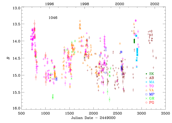
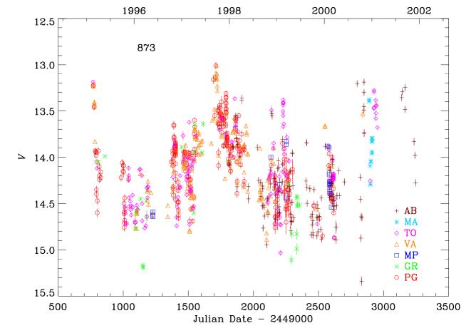
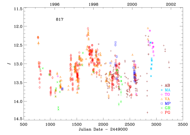
The light curves in the Johnson’s $BV$ and Cousins’ $RI$ bands are shown in Figs. 1–4, where different symbols (and colours) refer to the various telescopes listed in Table 1. All our $UBVRI$ CCD data are reported in Tables 3–7, available in electronic form.

Figure 1: Light curve of S5 0716+71 in the $B$ band

Figure 2: Light curve of S5 0716+71 in the $V$ band

Figure 3: Light curve of S5 0716+71 in the $R$ band; the BeppoSAX pointing of October 30, 2000 is indicated by the vertical line; the dashed line represents a cubic spline interpolation through the binned light curve (200 days), excluding the last, undersampled observing season; dotted lines are obtained by shifting the above spline by $\pm 0.75\,\rm mag$ in order to define a $1.5\,\rm mag$ constant variation area

Figure 4: Light curve of S5 0716+71 in the $I$ band

Table 3: $U$ data

$\rm JD-2449000$	$U$	Error	Observatory

Table 4: $B$ data

$\rm JD-2449000$	$B$	Error	Observatory

Table 5: $V$ data

$\rm JD-2449000$	$V$	Error	Observatory

Table 6: $R$ data

$\rm JD-2449000$	$R$	Error	Observatory

Table 7: $I$ data

$\rm JD-2449000$	$I$	Error	Observatory

The high declination of the source allows a quasi-continuous monitoring during the year, reducing time gaps due to the solar conjunction. However, technical reasons as well as bad weather conditions caused poor sampling during the last observing seasons.

The lack of dense overlapping among the datasets coming from the eight participating observatories prevents a safe determination of possible magnitude offsets due to the use of different photometric systems and/or different reduction procedures. However, when data from different telescopes are available during the same night the agreement is satisfactory.

Light curves appear as the superposition of fast flares lasting a few days on a modulated base level oscillating on year time scale. Four major optical outbursts were detected at the beginning of 1995, in late 1997, at the end of 2000, and in fall 2001. In the second-last outburst the source brightness reached a maximum of $R=12.54\pm 0.01$ on $\rm JD=2451877.63$.

We notice that in the first six observing seasons the long-term variation amplitude is roughly constant, about 1.5 mag, the trend traced by the minima being very similar to that traced by the maxima. This can be seen more easily in Fig. 3, where the dashed line represents the result of a cubic spline interpolation through the best-sampled $R$-band light curve (after binning with a 200 day bin size), while the dotted lines are obtained by shifting the spline by $\pm 0.75\,\rm mag$. The last, very undersampled observing season was excluded from the spline interpolation. By considering the different sampling density in the various observing seasons, one can say that the constant-amplitude area defined by the dotted curves contains, in a satisfactory way, all data up to $\rm JD\sim 2451800$; on the contrary, in the 2000–2001 observing season the variation amplitude is much larger, exceeding 2 mag. In particular, a spectacular brightness increase of 2.3 mag in 9 days was detected in October 2000, from $R=14.88\pm 0.03$ on $\rm JD=2451830.561$ observed from Abastumani, to $R=12.55\pm 0.02$ on $\rm JD=2451839.553$ observed from Vallinfreda. This is one of the strongest variations ever detected not only for this source but more in general for the blazar class. The impressive brightening of the source triggered the ToO observation of the X-ray satellite BeppoSAX performed on October 30 (see Sect. 4.2).

Notice also that the time separation between the $R$ brightness minima registered on $\rm JD=2450153$ and $\rm JD=2451208$ is about the same (1055 days, corresponding to $\sim 2.89$ years) which holds between the maxima on $\rm JD=2450710$–2450717 and $\rm JD=2451839$–2451877. Actually, a similar time separation ($\sim 2.65$ years) is also found between the peak at $\rm JD=2450710$–2450717 and that at $\rm JD=2449727$–2449767. Although this is obviously a sampling-biased finding, nonetheless it suggests that a sort of recurrent behaviour may characterize the 0716+714 optical light curve. Of course, this major point requires a more robust analysis, which will be performed in Sect. 6.

Table 1 also presents some statistics on the optical fluxes: these were obtained from magnitudes by correcting for a Galactic extinction of 0.081, 0.070, 0.053, 0.045, and 0.032 mag in $UBVRI$, respectively, and by using the absolute flux densities for zero mag given by Bessell (bes79 (1979)). Mean fluxes $<$$F$$>$ and standard deviations $\sigma$, in mJy, are reported, together with the mean fractional variation, defined as $f_{\rm var}=\sqrt{\sigma^{2}-\delta^{2}}/$$<$$F$$>$, where $\delta^{2}$ is the mean square uncertainty of the fluxes (Peterson pet01 (2001)). In general, $f_{\rm var}$ increases with sampling, which makes a comparison among different bands difficult to perform. One can only say that the mean fractional variation is around 40% in all the optical bands.

4.1 Colour indices

The existence of spectral changes possibly related to flux variations was investigated by analyzing colour indices. We first derived weighted mean colour indices by coupling the most precise data (errors not greater than 0.05 mag in $UB$ and 0.04 mag in $VRI$) taken by the same instrument within 30 minutes. The results are shown in Table 8, which also reports the standard deviation of the sample $\sigma$ and the number of indices $N$ derived. As one can expect, in general the standard deviation increases with the frequency separation between the two bands, the largest value corresponding to the $B-I$ index.

Table 8: Statistics of colour indices

Index	Mean	$\sigma$	$N$
$U-B$	$-0.554$	0.018	13
$B-V$	$0.434$	0.062	444
$B-R$	$0.889$	0.056	780
$B-I$	$1.382$	0.097	356
$V-R$	$0.420$	0.044	561
$V-I$	$0.937$	0.059	458
$R-I$	$0.524$	0.052	522

Then we concentrated on the $B-R$ index, the best sampled one. Its behaviour versus time is shown in Fig. 5 (top panel), where it is compared with the light curve in the $R$ band (bottom panel). One can see that the colour index is indeed variable, but the spectral changes do not follow the long-term brightness variations.

Figure 5: Temporal evolution of the $B-R$ index (top) compared with the $R$ light curve (bottom); the dashed (red) line in the top panel indicates the average value $B-R=0.889$

Indeed, when analyzing the data of the 1995–1996 observing season, Ghisellini et al. (ghi97 (1997)) found that “The colour index correlates with intensity during the rapid flares (the spectrum is flatter when the flux is higher), but it is rather insensitive to the long term trends.”. The “achromatic” nature of the long-term flux oscillations was also recognized by Villata et al. (vil02 (2002)) in their analysis of the optical behaviour of BL Lacertae during the 2000–2001 WEBT campaign.

If we calculate the mean $B-R$ for each observing season, we see that it is almost constant, around 0.84 mag, before $\rm JD\sim 2451000$, while it jumps to about 0.91 after that date, staying at that level for the subsequent three seasons (the last season is too undersampled to be included in this analysis). This transition to a steeper spectral state seems to occur during the dimming phase of the big outburst peaking in late 1997.

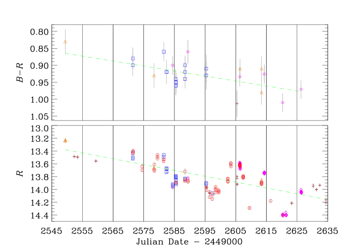
On a shorter time scale, a spectral steepening corresponding to a brightness decrease is also evident in the period $\rm JD\sim 2451545$–2451630 (see Fig. 6, where linear fits have been plotted to guide the eye).

Figure 6: Temporal evolution of the $B-R$ index (top) compared with the $R$ light curve (bottom) in the last part of the sixth observing season; linear fits and vertical lines have been plotted to guide the eye; symbols as in Figs. 1–4

On even shorter time scales, different behaviours have been found: sometimes a bluer-when-brighter trend is recognizable, while in some other cases the opposite is true; there are also cases where magnitude variations do not imply spectral changes. We think that a very dense monitoring with high-precision data is needed to safely distinguish trends in the short-term spectral behaviour of this source.

The analysis of the other colour indices leads to similar results.

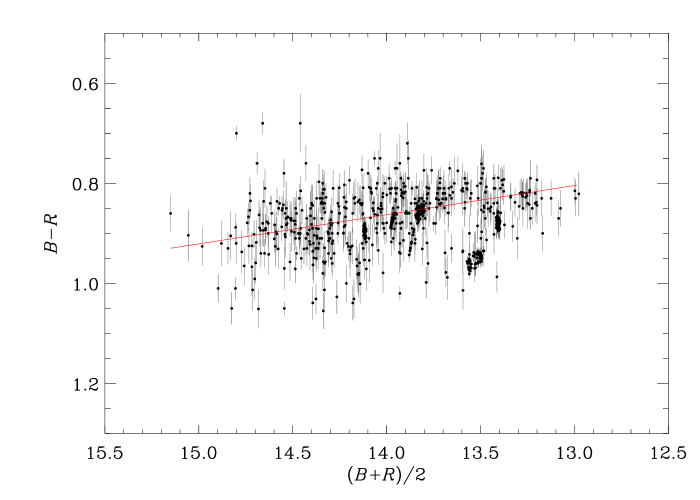
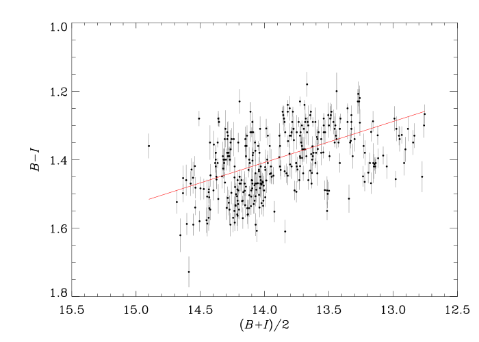
The existence of a more general correlation between colour index and brightness level can be checked by looking at Fig. 7, where $B-R$ is plotted versus $(B+R)/2$ in order to minimize the bias introduced by the dependence of the colour index on the magnitudes that are used to calculate it (Massaro & Trèvese mas96 (1996)). A linear fit was drawn after averaging the colour indices obtained during the same night; its slope of $0.058\pm 0.003$ and the linear Pearson correlation coefficient $r=0.15$ suggest a weak correlation between colour index and brightness. The bluer-when-brighter correlation becomes clearer when plotting $B-I$ against $(B+I)/2$ (Fig. 8), because of the larger frequency separation between $B$ and $I$. In this case the slope of the linear fit is $0.120\pm 0.004$ and $r=0.44$.

Figure 7: The $B-R$ index as a function of $(B+R)/2$; the linear fit was obtained after averaging data of the same night

Figure 8: The $B-I$ index as a function of $(B+I)/2$; the linear fit was obtained after averaging data of the same night

One can then wonder how much data inhomogeneities due to the fact that we are working with different datasets may affect our conclusions. In order to check the influence of systematic offsets we derived weighted mean $B-R$ values for each observatory (see Table 9, which also gives $\sigma$, $N$, and the deviation $\Delta$ from the average value 0.889 obtained by including data from all observatories). As one can see, large deviations from the average value of 0.889 are found only for the Greve and Perugia mean values, which are derived from a small number of $BR$ couples. In particular, all the Perugia indices come from data of the first observing season, when $B-R$ was intrinsically lower than average (see Fig. 5). The not negligible deviation of the Skinakas data may be due to the fact that all of them were taken in the same night, when the colour index might have been far from its average value. The same sampling problem also holds for the Mount Maidanak values, all coming from the same observing season. In this case, however, the deviation from the average value is quite small.

Table 9: Weighted mean $B-R$ values from each observatory, their standard deviation $\sigma$, their number $N$, and their deviation from the weighted mean value of 0.889 reported in Table 8

Observatory	$<$$B-R$$>$	$\sigma$	$N$	$\Delta$
Greve	0.766	0.085	17	$-0.123$
Perugia	0.779	0.037	8	$-0.110$
Vallinfreda	0.852	0.054	166	$-0.037$
Monte Porzio	0.912	0.036	23	$0.023$
Abastumani	0.896	0.069	79	$0.007$
Torino	0.858	0.055	207	$-0.031$
Skinakas	0.953	0.011	53	$0.064$
Mt. Maidanak	0.878	0.018	227	$-0.011$

The deviations $\Delta$ from the average value 0.889 were then used to “correct” the colour indices of each observatory, in order to see whether “normalized” indices may reveal a clearer spectrum-brightness correlation with respect to that shown by the original data. No shift was assigned to the Skinakas, Perugia, and Maidanak data, since they refer to very limited time intervals, as discussed above. The result is very similar to what was obtained without “normalization”, leading to the conclusion that the possible existence of systematic colour-index offsets among different observatories does not affect the general bluer-when-brighter weak correlation.

4.2 Observations during the BeppoSAX pointing

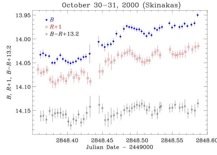
The BeppoSAX ToO pointing activated on October 30, 2000 found the source in a relatively bright optical state. The observations carried out at the Skinakas Observatory during that night are shown in Fig. 9, where $B$ and $R$ light curves are plotted together with the $B-R$ colour index. Exposure times of 120 s in $B$ and 60 s in $R$ were adopted.

The total magnitude variation was not exceptional, about 0.1 mag. In general, the behaviour in the $B$ band is better defined, especially in the first part of the curve. The $B$ and $R$ light curves follow a similar behaviour, and the colour index seems to present some correlation with brightness, similar to that already seen by Villata et al. (vil00 (2000)), i.e. with a slight delay in colour changes (see in particular the central peak of the curves).

Figure 9: $B$, $R$ ($+1$), and $B-R$ ($+13.2$) curves of October 30–31, 2000, simultaneous with the BeppoSAX pointing; data are from the Skinakas Observatory

4.3 Comparison with the Qian et al. (qia02 (2002)) data

Qian et al. (qia02 (2002)) have recently published Johnson’s $BV$ and Cousins’ $RI$ data from November 1994 to March 2000 taken with the 1.56 m telescope of the Sheshan Station of the Shangai Astronomical Observatory. Fig. 10 compares our data in the $R$ and $I$ bands (black dots) with theirs (grey open circles, green in the electronic version).

Figure 10: Comparison between data from this paper (black dots) and those by Qian et al. (qia02 (2002); grey open circles, green in the electronic version) in the $R$ (top) and $I$ (bottom) bands

By a first look, the Qian et al. (qia02 (2002)) data show a total magnitude variation much larger than what we detected in our eight observing seasons. In particular, one can notice that the most evident disagreement is due to some data points (their brightness maxima) at a peculiarly stable magnitude ($V\sim 12.5$, $R\sim 12.1$, $I\sim 11.8$), very similar to that of one of the reference stars used by them. As a consequence, they found extremely strong intraday variations, such as that of more than 2 mag in the $R$ band in 21 hours on $\rm JD=2451536$–2451537 and the 1.84 mag dimming in $I$ band in 40 min a couple of days before (even if there is disagreement on this latter variation between the printed and the electronic versions of the data table). They also report several other surprising intranight variations, of the order of half a mag in few minutes.

5 Radio light curves

The complete radio flux-density light curves (Jy) obtained by the four radio telescopes participating in the present work are plotted in Fig. 11. They include data taken by the Metsähovi Radio Observatory (37 and 22 GHz), starting from 1988, observations performed by UMRAO (14.5, 8.0, and 4.8 GHz), dating back to 1981, data obtained with the Effelsberg radio telescope (43, 32, 23, 15.0, 10.7, 8.4, 5.0, 2.7, 1.7, and 1.4 GHz) since 1978, and observations done at the Pico Veleta radio telescope (230, 150, and 90 GHz), starting from 1983. Data at 5, 8.4, and 22 GHz published by Venturi et al. (ven01 (2001)) are also shown.

In order to obtain better sampled light curves, we combined data at similar frequencies: observations at 22 GHz published by Venturi et al. (ven01 (2001)) were added to those at the same frequency from Metsähovi and to the 23 GHz ones from Effelsberg; data at 15.0 GHz from Effelsberg were considered together with those at 14.5 GHz from UMRAO; another combined light curve was obtained by assembling the 8.0 GHz data from UMRAO with the 8.4 GHz ones from Effelsberg and Venturi et al.; finally, 5.0 GHz data from Effelsberg and 5 GHz ones (actually including 4.9 and 5.0 GHz observations) from Venturi et al. were put together with the 4.8 GHz data from UMRAO. Moreover, the 230, 150, 90, 43, 37, 32, 2.7, 1.7, and 1.4 GHz data are shown in Fig. 11 in three panels only, in order to save space; the 10.7 GHz flux densities are in the same panel of the 8.0–8.4 GHz light curve.

Figure 11: The complete radio light curves from the Metsähovi Radio Observatory, UMRAO, Effelsberg and Pico Veleta radio telescopes; in the 14.5–15.0 GHz plot the (red) dotted line indicates the trend which was removed in the statistical analysis; data from Venturi et al. (ven01 (2001)) are also added

The most extended and best sampled light curves at 15 (14.5–15.0), 8 (8.0–8.4), and 5 (4.8–5.0) GHz seem to suggest an almost linear decrease of the base-level flux from the starting date until 1995.

The oldest data at 8 (and 5) GHz witness a high state of the source before 1980, followed by a phase of moderate activity. After 1984 data become rather sparse up to mid 1993. In this period outbursts seem to have occurred in late 1985, 1986–1987, 1988, and 1992. After that time, an epoch of essentially low radio brightness can be identified, lasting until early 1998 (see also Fig. 12). During this period, the radio-flux mean level is roughly the same at all wavelengths, about 0.5 Jy. Then the radio flux started a fast rise, leading to a big outburst, which was characterized by flaring activity. After more than one year, in mid 1999 the flux was slowly declining, and at the end of the observing period it was more or less back to the pre-outburst level.

Figure 12: Optical (top panel, mJy) and radio (Jy) flux light curves from 1994 to 2001; vertical dashed lines are drawn to guide the eye through the major optical flares

On top of this common behaviour, one has to notice that the variation amplitude of the radio flux decreases with increasing wavelength, a feature which is often found in sources of this kind (e.g. Aller et al. all85 (1985)). Moreover, there may be a delay of the lower-frequency flux changes with respect to the higher-frequency ones, which needs to be confirmed by a cross-correlation analysis (see Sect. 6.3).

We notice that there are four maximum points in the 14.5 GHz UMRAO light curve (red diamonds in Fig. 11) that are separated by a time interval of about 2000–2100 days. This would suggest a characteristic time of variability of 5.5–5.7 years for the radio fluxes of 0716+714, which will be checked in the next section.

Table 10 contains some statistics on the best sampled light curves: the total number of data $N$, the mean flux $<$$F$$>$, the standard deviation $\sigma$, and the mean fractional variation $f_{\rm var}$ already defined for the optical fluxes. In general, there is a decreasing trend of $<$$F$$>$, $\sigma$, and $f_{\rm var}$ with decreasing frequency. Notice that, while in the optical bands $f_{\rm var}$ is almost constant and around 0.4 (see Table 1), in the radio band it varies substantially with frequency, reaching values much higher than the optical ones.

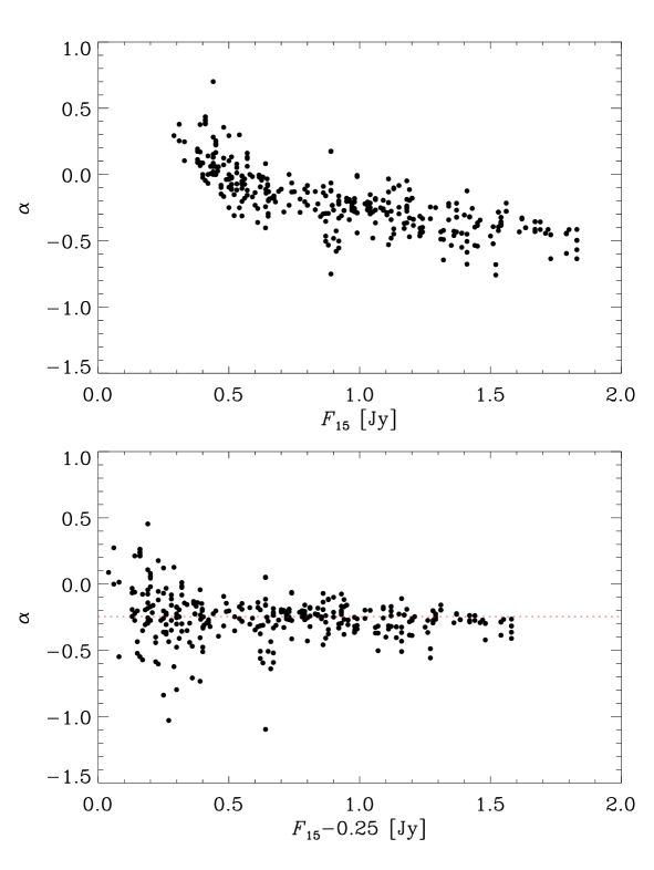
This frequency-dependent behaviour seems to be mainly ascribable to the presence of a flux base level which, unlike the variation amplitude, does not dim with increasing wavelength. This suggests that the observed radio flux could be the sum of two different contributions: the strongly variable flux coming from the jet would be superposed to a stabler component, possibly coming from more extended jet regions, or from a steady radio core, or from elsewhere. The two components would have rather different spectra: the variable component being harder than the base-level one. Thus, the observed resulting spectrum would vary according to which component dominates. This feature is evident in the top panel of Fig. 13, where the 5-15 GHz spectral index $\alpha$ ($F_{\nu}\propto\nu^{-\alpha}$) is plotted versus the 15 GHz flux. Indeed, a chromatic behaviour can be recognized, the spectrum becoming harder when the flux increases, i.e. when the variable component dominates. In the bottom panel we try to separate the two contributions by subtracting a base-level flux of 0.25 and 0.35 Jy from the 15 and 5 GHz data, respectively: an essentially achromatic behaviour is obtained, points being distributed around the mean value $\alpha=-0.25$ (red dotted line). One can thus conclude that two components with different spectra and achromatic behaviour may indeed be present in the observed radio fluxes of S5 0716+71, whose combination gives rise to the observed flux-dependence of the radio spectral index. According to this interpretation, the long-term spectral behaviour of the variable radio component would be consistent with the essentially achromatic optical one (see Sect. 4.1).

Figure 13: Top: spectral index between the 5 and 15 GHz radio bands versus the 15 GHz flux. Bottom: the same as in the top panel after subtracting the base levels from the fluxes (see text)

Table 10: Statistics of radio data at different frequencies $\nu$

$\nu$ [GHz]	$N$	$<$$F$$>$ [Jy]	$\sigma$ [Jy]	$f_{\rm var}$
22–23	183	1.12	0.62	0.66
14.5–15.0	527	0.88	0.42	0.61
8.0–8.4	374	0.86	0.33	0.47
4.8–5.0	506	0.71	0.26	0.30

6 Statistical analysis

6.1 Characteristic time scales of variability

A number of blazars have revealed a periodic or quasi-periodic flux behaviour in the optical and/or radio bands, with various time scales, ranging from a few days to more than 10 years. Examples of long-term cycles are the $\sim 12$ year period observed in the OJ 287 optical light curve (Sillanpää et al. sil88 (1988), sil96 (1996); Villata et al. 1998b ), the $\sim 7.8$ year period discovered in the optical light curve of BL Lacertae (Smith & Nair smi95 (1995); Marchenko et al. mar96 (1996)), and the $\sim 5.7$ year period recognized in the radio light curves of AO 0235+16 (Raiteri et al. rai01 (2001)). More in general, Smith et al. (smi93 (1993)) and Smith & Nair (smi95 (1995)) found that many AGNs display smooth, cyclic changes in level on time scales of years. The BL Lac object 0716+714 was not examined by them, since it was not included in the Rosemary Hill Observatory AGN monitoring program they were referring to. As mentioned in Sect. 2, hints for a short-term (a few days) periodic behaviour of the 0716+714 optical light curve were found by Heidt & Wagner (hei96 (1996)) and by Qian et al. (qia00 (2000)).

In this section we are going to search for characteristic time scales of variability of S5 0716+71 in both the optical and radio bands. Beyond the visual inspection of the light curves, a number of statistical tools will be applied, such as the Discrete Fourier Transform (DFT; see e.g. Press et al. pre92 (1992)), the Discrete Correlation Function (DCF; Edelson & Krolik ede88 (1988); Hufnagel & Bregman huf92 (1992)), and the Structure Function (SF; Simonetti et al. sim85 (1985)). It is common usage to remove a possible linear trend from the datasets before processing them. In the case of 0716+714, no linear trends can be recognized in the optical light curves, while a smooth flux decrease is clearly visible in the UMRAO light curves up to $\rm JD\sim 2450000$ (see Fig. 11).

Application of the DFT leads to a power spectrum, whose peaks may indicate the existence of sinusoidal components in the light curve. We first applied the Fourier analysis to the optical fluxes; the $R$ flux (mJy) light curve is displayed in Fig. 12 (top panel); data taken in 1994 by Sagar et al. (sag99 (1999)) have been added to extend it in time.

The DFT applied to the $R$ fluxes binned over 20 days gives only one strong signal at a frequency of $8.175\times 10^{-4}\,\rm days^{-1}$, corresponding to a period of 1223 days; its false-alarm probability, which represents the probability that the data values are independent Gaussian random values, is only $3.08\times 10^{-7}$ (see Fig. 14, top panel, where the dotted line represents the confidence level of $10^{-3}$).

The reliability of this result was then checked by performing the autocorrelation analysis of the $R$ fluxes by means of the DCF. The original fluxes were binned over 10 days and the DCF calculated by sampling over 40 days. In this way spurious effects, which depend on the inverse square root of the number of points in each DCF bin, are constrained within 10%. The result is plotted in the middle panel of Fig. 14: the DCF shows a peak at a time lag of 1160–1240 days.

Finally, we calculated the SF, which gives an estimate of the mean flux difference as a function of time separation. If a periodic, symmetric signal does exist in the light curve, whose time scale is $P$, the SF will show alternate maxima and minima at $nP/2$, where $n$ are odd and even integers, respectively. The bottom panel of Fig. 14 displays the SF obtained with a bin size of 60 days: minima are found at 1225 and 2234 days, maxima at 573 and 1770 days, thus confirming the $\sim 1200$ day characteristic time scale of variability for the long-term trend of 0716+714 already suggested by the DFT and DCF analyses.

Indeed, a visual inspection of Fig. 3 (or Fig. 12) reveals that this time interval is similar to the time separation between the maximum brightness states observed in 1997 and late 2000 (see also Sect. 4).

Because of the limited time coverage of the data used for the present analysis ($\sim 2800$ days) in comparison with the time scale derived, it goes without saying that further monitoring is needed to check whether long-term flux changes repeat regularly every $\sim 3.3$ years.

Figure 14: Application of statistical techniques to the $R$ band fluxes of 0716+714: Discrete Fourier Transform periodogram as a function of frequency (top, the dotted line indicates the level above which the significance is better than 0.001), Discrete Correlation Function (middle) and Structure Function (bottom) versus time lag

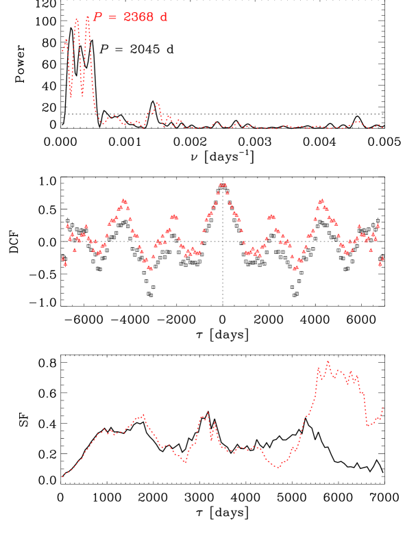
We performed the same analysis on the radio light curve obtained by adding the 15.0 GHz Effelsberg data to the 14.5 GHz UMRAO ones. This “15 GHz” light curve extends for about 7500 days, from early 1981 to late 2001. We applied the DFT, DCF, and SF methods first on the original fluxes (case 1) and then after subtracting the trend shown in Fig. 11: a linear decrease of slope $\sim-1.34\times 10^{-4}\,\rm Jy\,days^{-1}$ up to $\rm JD=2450000$, and a constant value of $\sim 0.47$ Jy from then on (case 2).

The results are shown in Fig. 15: black lines in the DFT (top) and SF (bottom) plots refer to case 1 (original data); the (red) dotted lines to case 2 (data corrected for the trend). In the DCF plot (middle) black squares refer to case 1 and (red) triangles to case 2. The DFT analysis reveals that in both cases there are three strong signals and two minor ones whose significance is better than 0.001 (dotted line in the top panel). In case 1 they correspond to time scales of 6427, 3214, 2045, 1500, and 703 days; in case 2 the first peak exceeds the time extension of the light curve and is due to the numerical frequency oversampling adopted (Press et al. pre92 (1992)), while the other time scales are 4090, 2368, 738, and 672 days. A recurrent time scale of 2045 days would confirm the 2000–2100 day periodicity suggested by the visual inspection of the light curve performed in Sect. 5. The results of the DCF analysis partially confirm the DFT findings, showing peaks around 2100 days and 4200–4300 days, weak in case 1 and more pronounced in case 2. The fact that the time lag corresponding to the latter peak is twice that of the former one suggests that there is indeed some recurrent behaviour. Finally, the SF does not show very pronounced minima for time lags around 2000–2400 days, even if an alternance of maxima and minima with $P\sim 2100$–2200 days in case 1 and a couple of deep minima with $P\sim 2350$–2700 days in case 2 seem to be consistent with the previous findings. The large discrepancy between the two cases around $\tau=6000$ days is due to the much greater prominence acquired by the 1998–2000 outburst in case 2.

Figure 15: Application of statistical techniques to the 15 GHz light curve of 0716+714: Discrete Fourier Transform periodogram as a function of frequency (top, the dotted line indicates the level above which the significance is better than 0.001), Discrete Correlation Function (middle) and Structure Function (bottom) versus time lag. Black solid lines and squares refer to case 1 (original data); (red) dotted lines and triangles to case 2 (data corrected for the trend shown in Fig. 11)

The same kind of analysis has been performed on the combined 5 GHz light curve, containing the 4.8 GHz data from UMRAO, the 5.0 GHz data from Effelsberg, and the 5 GHz data published by Venturi et al. (ven01 (2001)). The results are shown in Fig. 16. No linear trend was subtracted in this case, since the long-term light curve at this frequency shows only a weak indication of linear flux decrease (see Fig. 11). The periodogram in the top panel of Fig. 16 shows a strong peak corresponding to a period of 2174 days; peaks at 2100–2200 and 4100–4200 days are evident in the DCF plot (middle panel), while minima corresponding to similar time scales (and related maxima) are found in the SF plot (bottom panel).

Figure 16: Application of statistical techniques to the 5 GHz light curve of 0716+714: Discrete Fourier Transform periodogram as a function of frequency (top, the dotted line indicates the level above which the significance is better than 0.001), Discrete Correlation Function (middle) and Structure Function (bottom) versus time lag.

The same analysis performed on the 8 GHz combined light curve gives similar, but noisier results.

In conclusion, the analysis of the best-sampled combined datasets at 15, (8,) and 5 GHz, spanning more than 20 years, suggests that a periodic or quasi-periodic component with time scale of 5.5–6 years may exist in the radio light curves of 0716+714. This is the same time scale which characterizes the recurrence of the major radio outbursts of another BL Lac object: AO 0235+16 (Raiteri et al. rai01 (2001)).

As for the short-term flux variations, the statistical analysis run on the optical fluxes was not able to reveal any characteristic time scale, even when fluxes were cleaned from the contribution of the long-term trend oscillating with a $\sim 3.3$ year time scale.

6.2 Optical-radio correlation

Figure 12 compares the $R$-band fluxes (mJy, top panel) with the radio ones (see Fig. 11) in the period from 1994 to 2001.

An overall inspection of the light curves in Fig. 12 reveals that the behaviour of the radio fluxes is quite different from the optical one: there is not correspondence between the major optical events and the radio ones.

As mentioned in the Introduction, the existence of correlation between the optical and radio long-term trends has been investigated for a number of blazars: sometimes simultaneous flux variations in the two bands are found; in other cases correlation appears, but with a time delay, the optical variations usually leading the radio ones (see e.g. Tornikoski et al. tor94 (1994); Clements et al. cle95 (1995); Raiteri et al. rai01 (2001)).

We performed cross-correlation analysis between the optical fluxes and the 15 GHz combined dataset by means of the DCF; the result is shown in Fig. 17 (top panel) and was obtained by first binning the original data every 10 days, and then choosing a bin size for the DCF of 80 days. In this way a smooth plot is obtained and at the same time spurious effects are constrained to less than 5%. A first DCF maximum, indicating a possible correlation, appears at a time lag $\tau\sim-1000$–$-800$ days. The peak is found at $\tau=-960$ days and its DCF value is 0.48. A second, less pronounced maximum is found at $\tau\sim 200$–500 days. The value of the peak is 0.30 and corresponds to a time lag of 400 days. In the former case, a negative $\tau$ means that radio variations lead the optical ones, while in the other case the vice versa occurs. The signal at $\tau\sim-1000$–$-800$ days derives from connecting the radio outbursts occurred in 1992, early 1995, and 1998–1999 with the optical outbursts detected in early 1995, late 1997, and end 2000 – late 2001, respectively, while that at $\tau\sim 200$–500 days mainly comes from coupling the late-1997 optical outburst with the big radio outburst of 1998–1999. In order to obtain a more reliable estimate of the time lag, it is common usage to calculate the centroid of the DCF, $\tau_{\rm c}=(\sum_{i}\tau_{i}{\rm DCF}_{i})/(\sum_{i}{\rm DCF}_{i})$, where sums run over the points which have a DCF value close to the peak one. The centroids of the two DCF maxima in Fig. 17 are $-887$ and 364 days. We notice that, however, the low values of the DCF corresponding to both peaks indicate weak correlation between optical and radio variations.

Figure 17: Top: DCF between the optical and 15 GHz fluxes (open squares); red crosses show the mean DCF obtained after averaging 1000 Monte Carlo FR/RSS realizations. Bottom: CCPD for the negative-$\tau$ (left) and positive-$\tau$ (right) peaks of the DCF

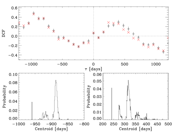
In order to check uncertainties in cross-correlation lags, we applied the Monte Carlo technique known as “flux redistribution/random subset selection” (FR/RSS; Peterson et al. pet98 (1998)). Random subsets of the two datasets to be correlated are selected, redundant points are discarded, and random Gaussian deviates constrained by the flux errors are added to the fluxes; the two subsets are then cross-correlated and the resulting DCF centroid stored. After cross-correlating $N$ Monte Carlo realizations of the two datasets, an average DCF can be calculated and compared with the original one. Moreover, a cross-correlation peak (actually, the centroid) distribution (CCPD) is obtained, from which a measure of the lag uncertainty can be derived. In this way a test is performed on the influence of both sampling and errors on the results.

We thus run FR/RSS processes with $N=1000$ to test the importance of the two DCF signals in the optical - 15 GHz cross-correlation. The average DCF is superposed to the original one in Fig. 17 (red crosses): all points but a few ones are inside the original DCF uncertainties. One interesting feature is that the simulations give more strength to the lower-$\tau$ part of the optical-leading DCF maximum, evidentiating the complexity of this signal. The resulting CCPDs are shown in Fig. 17 (bottom panels); as for the radio-leading signal, one can derive that at 76.6% confidence level the lag is in between $-896$ and $-877$ days and that at $1\sigma$ (see Peterson et al. pet98 (1998)) it is $-887^{+7}_{-5}$ days. The situation regarding the optical-leading signal is more complex: the time lag estimated from the original DCF falls in a tail of the probability distribution, while the Monte Carlo simulations indicate a lag between 304 and 331 days at 64.6% confidence level. This means that we are in the presence of a signal which actually results from the overlapping of different signals.

In any case, the weakness of the DCF maxima, their complexity, and especially the very large time delays which they would imply make us conclude that there is not a reliable radio-optical correlation in this source.

Another interesting feature in Fig. 17 is that there is only a very weak signal at zero time lag, which means that strong events in the optical (radio) band do not have a strong counterpart in the radio (optical) band.

However, it is worth performing a deeper visual inspection of the light curves in order to see if there is any (although weak) radio signature simultaneous with the optical outbursts. In order to analyse this point, dashed vertical lines are drawn in Fig. 12 to guide the eye through the major optical peaks. As for the first, double-peaked outburst of 1995, one can only notice that a modest radio peak is recognizable in the 37–43 GHz light curves, and a slightly delayed flux enhancement is visible in the 15 and 8 GHz light curves.

The few radio data available around the period when the big optical outburst of late 1997 occurred witness an enhanced flux with respect to the surrounding mean level.

The two less prominent optical peaks detected at the end of 1998 and the beginning of 1999 occurred during the big radio outburst, so it is difficult to look for their possible signature in the radio light curves. However, an enhanced radio flux is visible in correspondence to the 1999 flare at 22–23 and 15 GHz.

Finally, also the double-peaked optical outburst observed at the end of 2000 may have a modest radio counterpart, as the millimetric light curves (second panel from the top in Fig. 12) seem to suggest, even if the radio sampling at that time is rather sparse.

In conclusion, one can say that a modest radio flux increase may correspond to a major optical outburst. However, we warn that this hypothesis must be considered with caution because of insufficient data sampling.

By cross-correlating the optical fluxes with the other combined radio light curves at 5, 8, and 22–23 GHz, one gets essentially the same results, but the values of the two DCF maxima increase when cross-correlating higher-frequency radio light curves since, as seen in Sect. 5, the higher the frequency the larger the variation amplitude.

Different results are instead obtained when investigating the optical-millimetric correlation: many signals are obtained, but the small number of millimetric data prevents a reliable analysis to be performed. Further intense monitoring at the higher radio frequencies is a major need in order to better understand the source multiwavelength behaviour.

6.3 Radio-radio correlations

As already noticed, by looking at Figs. 11 and 12 it is evident that all the radio bands exhibit a similar behaviour, even if flux variations become smaller and smaller when going from the highest to the lowest radio frequencies. This is a rather common feature in blazars; moreover, it is often found that radio variations at the lower frequencies lag those at the higher frequencies (see e.g. Aller et al. all85 (1985), all99 (1999); Tornikoski et al. tor94 (1994); Raiteri et al. rai01 (2001)). In order to investigate this point, in this section we perform cross-correlation analysis between fluxes at different radio wavelengths by means of the DCF method.

The result of cross-correlating the 22–23 GHz and 15 GHz datasets is presented in Fig. 18 (left panel).

Figure 18: Left: cross-correlation between the 22–23 and 15 GHz data. Right: CCPD relative to the central peak obtained by running 1000 FR/RSS Monte Carlo realizations

The four most significant maxima are found at time lags of $\sim-150$, $\sim-50$–$-30$, $\sim 0$–20, and $\sim 150$ days. In particular, the peak at $\tau\sim 0$–20 days suggests that flux variations at 15 GHz may be delayed with respect to those at 22–23 GHz by some days. The lack of a better sampling does not allow us to improve the $\tau$ resolution of the plot without increasing too much spurious effects, which are now constrained to a few percents. Calculation of the centroid for the central peak gives $\tau_{\rm c}=7$ days. Its CCPD is shown in the right panel of Fig. 18: from it one can derive that at the 99.8% confidence level the time delay is 6–9 days, which is significantly different from zero, i.e. we can conclude that flux variations at 15 GHz do lag those at 22–23 GHz.

An indication of a larger delay is found by cross-correlating the 22–23 GHz data with the 8 GHz ones. The result is shown in Fig. 19 (left panel): the peak is found at $\tau=15$ days, but the centroid gives a time lag of 22 days. The CCPD (right panel) allows one to derive that at $1\sigma$ $\tau=22\pm 2$ days.

Figure 19: Left: cross-correlation between the 22–23 and 8 GHz data. Right: CCPD relative to the central peak obtained by running 1000 FR/RSS Monte Carlo realizations

We finally tested the correlation between the 15 and 5 GHz fluxes. As can be seen in Fig. 20 (left panel) the result is again a delay, the DCF peaking at $\tau=45$ days, while $\tau_{\rm c}=53$ days. The CCPD confirms the reliability of this delay (see Fig. 20, right panel): the time lag is $\tau=53\pm 2$ days at 93% confidence level.

Figure 20: Left: cross-correlation between the 15 and 5 GHz data. Right: CCPD relative to the central peak obtained by running 1000 FR/RSS Monte Carlo realizations

The above results suggest that the flux variations at the lower radio frequencies are delayed with respect to those at the higher frequencies.

7 Conclusions

In this paper we have presented the most complete optical and radio light curves of the BL Lacertae object 0716+714 ever published. 4854 $UBVRI$ data were taken from eight observatories during eight observing seasons, from 1994 to 2001. Radio light curves from 1.4 to 230 GHz, most of which spanning more than 20 years, were obtained by four radio observatories.

A long-term trend is visible in the optical light curves, on which variations on shorter time scales are superposed; statistical analysis by means of DFT, DCF, and SF suggests that the long-term trend may oscillate on a $\sim 3.3$ year time scale, while no periodicity is found for the fast flux changes. The same analysis performed on the best-sampled combined datasets at 5, 8, and 15 GHz indicates that radio fluxes may have a variability time scale of 5.5–6 years. It is worth noticing that a similar period was recognized in the radio light curve of another BL Lac object: AO 0235+16 (Raiteri et al. rai01 (2001)).

During the first six observing seasons the variation amplitude of the optical light curves is roughly constant, about 1.5 mag, but in the 2000–2001 season a dramatic brightening of 2.3 mag in 9 days was observed, leading to an increase of the variability amplitude.

A constant variability amplitude in magnitudes implies a flux variation amplitude which is proportional to the flux level, and this can be easily explained in terms of a variation of the Doppler beaming factor $\delta=[\Gamma(1-\beta\cos\theta)]^{-1}$, where $\Gamma$ is the Lorentz factor of the bulk motion of the emitting plasma in the jet and $\theta$ is the viewing angle. In this framework, assuming that the intrinsic flux is relativistically enhanced by a factor $\delta^{3}$, the maximum oscillation of the long-term trend identified in Fig. 3 would imply a variation of $\delta$ of a factor $\sim 1.3$. This change could be due to either energetic or geometrical reasons, or to a combination of both. In a paper on the optical variability of BL Lacertae during the May 2000 – January 2001 WEBT campaign, Villata et al. (vil02 (2002)) favoured a geometrical interpretation. The case of 0716+714 is very similar, since a variation of a factor 1.3 of $\delta$ can be explained by a variation of few degrees of the viewing angle, while it would require a noticeable change of the Lorentz factor.

Colour analysis on the optical light curves reveals only a weak general correlation between the colour index and the source brightness. In at least one case a clear spectral steepening was observed during a long-lasting dimming phase; moreover, the optical spectrum after $\rm JD\sim 2451000$ is on the average redder than before, the change occurring in the decaying phase of the late-1997 outburst. On shorter time scales, different spectral behaviours were found.

Radio light curves at different frequencies have a similar behaviour, but the flux variation amplitude becomes smaller with decreasing frequency, a feature which is often observed in blazars (e.g. Aller et al. all85 (1985)). Unlike the essentially achromatic optical long-term behaviour, the radio spectrum becomes harder when the source brightens. However, this behaviour can be interpreted as due to the combination of two contributions with different spectra: a steady base level and a harder-spectrum variable component. Both contributions are achromatic, but the resulting spectrum varies according to which component dominates.

Cross-correlation between radio light curves indicates that, with a high degree of correlation, flux variations at lower frequencies lag the higher-frequency ones with time delays from a few days to several weeks, depending on the frequency separation. Again, this has already been observed for other blazars and has been interpreted in various ways. In the framework of a homogeneous model, where the radiation is produced in a single homogeneous blob relativistically moving at a small viewing angle, lags are interpreted in terms of electron cooling time scales. On the other hand, in an inhomogeneous jet the higher synchrotron frequencies are emitted from the inner, denser parts of the jet, while the lower ones are emitted from progressively more external regions. In this case, the time lag is a measure of the distance between emitting regions in the jet. Indeed, a perturbance travelling down the jet would trigger the emission of different frequencies at different times. Also in a rotating helical jet model the jet inhomogeneity causes time lags in the flux variations at diverse wavelengths, since the different-frequency emitting portions of the jet acquire the same viewing angle at different times (Villata & Raiteri vil99 (1999)).

Radio and optical light-curve behaviours appear quite different, the epochs where the broad radio outbursts are observed not corresponding to the periods when the faster optical outbursts are seen. However, minor radio flux enhancements are found simultaneously with the major optical outbursts, as if the mechanism causing the optical brightenings can only marginally affect the radio band, while another process not affecting the optical band is responsible for the dominant radio events. Moreover, the characteristic variability time scales of the two bands are different.

Indeed, cross-correlation analysis by means of the DCF gives only two weak signals at time lags of $\sim-887$ days and $\sim 364$ days. In the former case radio variations would lead the optical ones by about 2.4 years, a picture difficult to explain. The latter possibility, i.e. radio variations following the optical ones by about 1 year, would be more easily interpreted within the same scenarios which explain the radio-radio delays discussed above.

In any case, it is worth underlying that the cross-correlation analysis we performed found only weak correlation between the optical and radio emissions. This is very different from what was found for other BL Lac objects, such as AO 0235+16 (Raiteri et al. rai01 (2001)), which shows strong correlation between optical and radio bands, with short or even null time lag. This is an important difference that models explaining blazar variability should address.

• the NASA/IPAC Extragalactic Database (NED), which is operated by the Jet Propulsion Laboratory, California Institute of Technology, under contract with the National Aeronautics and Space Administration;

• data from the University of Michigan Radio Astronomy Observatory, which is supported by the National Science Foundation and by funds from the University of Michigan.

• observations with the 100 m telescope of the MPIfR (Max-Planck-Institut für Radioastronomie) at Effelsberg.

References

- (1) Aller H.D., Aller M.F., Latimer G.E., Hodge P.E., 1985, ApJS 59, 513
- (2) Aller M.F., Aller H.D., Hughes P.A., Latimer G.A., 1999, ApJ 512, 601
- (3) Antonucci R.R.J., Hickson P., Olszewski E.W., Miller J.S., 1986, AJ 92, 1
- (4) Bach U., Krichbaum T.P., Ros E., et al., 2002, in: Ros E., Porcas R.W., Lobanov, A.P., Zensus J.A. (eds.) Proc. 6th European VLBI Network Symposium, p. 119 (arXiv:astro-ph/0207083)
- (5) Bach U., et al., 2003 (in preparation)
- (6) Beskin G.M., Lyutyĭ V.M., Neizvestnyĭ S.I., Pustil’nik S.A., Shvartsman V.F., 1985, AZh 62, 432; SvA 29, 252
- (7) Bessell M.S., 1979, PASP 91, 589
- (8) Biermann P., Duerbeck H., Eckart A., et al., 1981, ApJ 247, L53
- (9) Bloom S.D., Marscher A.P., Gear W.K., et al., 1994, AJ 108, 398
- (10) Clements S.D., Smith A.G., Aller H.D., Aller M.F., 1995, AJ 110, 529
- (11) Edelson R.A., 1987, AJ 94, 1150
- (12) Edelson R.A., Krolik J.H., 1988, ApJ 333, 646
- (13) Gabuzda D.C., Kovalev Y.Y., Krichbaum T.P., et al., 1998, A&A 333, 445
- (14) Gabuzda D.C., Kochenov P.Yu., Cawthorne T.V., Kollgaard R.I., 2000, MNRAS 313, 627
- (15) Gear W.K., Robson E.I., Ade P.A.R., et al., 1984, ApJ 280, 102
- (16) Ghisellini G., Villata M., Raiteri C.M., et al., 1997, A&A 327, 61
- (17) Giommi P., Massaro E., Chiappetti L., et al., 1999, A&A 351, 59
- (18) González-Pérez J.N., Kidger M., Martín-Luis F., 2001, AJ 122, 2055
- (19) Heeschen D.S., Krichbaum Th., Schalinski C.J., Witzel A., 1987, AJ 94, 1493
- (20) Heidt J., Wagner S.J., 1996, A&A 305, 42
- (21) Hufnagel B.R., Bregman J.N., 1992, ApJ 386, 473
- (22) Impey C.D., Bychkov V., Tapia S., Gnedin Y., Pustilnik S., 2000, AJ 119, 1542
- (23) Jorstad S.G., Marscher A.P., Mattox J.R., et al., 2001, ApJS 134, 181
- (24) Kraus A., Quirrenbach A., Lobanov A.P., et al., 1999, A&A 344, 807
- (25) Kühr H., Pauliny-Toth I.I.K., Witzel A., Schmidt J., 1981, AJ 86, 854
- (26) Kurtanidze O.M., Nikolashvili M.G., 1999, in: Raiteri C.M., Villata M., Takalo L.O. (eds.) Proc. OJ-94 Annual Meeting 1999, Blazar Monitoring towards the Third Millennium. Osservatorio Astronomico di Torino, Pino Torinese, p. 25
- (27) Marchenko S.G., Hagen-Thorn V.A., Yakovleva V.A., Mikolaichuk O.V., 1996, PASPC 110, 105
- (28) Massaro E., Trèvese D., 1996, A&A 312, 810
- (29) Massaro E., Maesano M., Montagni F., et al., 1999, PASPC 159, 139
- (30) Nesci R., Massaro E., Montagni F., 2002, Publ. Astron. Soc. Aust. 19, 143
- (31) Ott M., Witzel A., Quirrenbach A., et al., 1994, A&A 284, 331
- (32) Peng B., Kraus A., Krichbaum T.P., Witzel A., 2000, A&AS 145, 1
- (33) Peterson B.M., 2001, in: The Starburst-AGN Connection 2001. World Scientific, Singapore (arXiv:astro-ph/0109495)
- (34) Peterson B.M., Wanders I., Horne K., et al., 1998, PASP 110, 660
- (35) Press W.H., Teukolsky S.A., Vetterling W.T., Flannery B.P., 1992, Numerical Recipes in Fortran - The Art of Scientific Computing. Cambridge University Press, Cambridge
- (36) Qian B., Tao J., Fan J., 2000, PASJ 52, 1075
- (37) Qian B., Tao J., Fan J., 2002, AJ 123, 678
- (38) Quirrenbach A., Witzel A., Krichbaum T., et al., 1989, Nat 337, 442
- (39) Quirrenbach A., Witzel A., Wagner S., et al., 1991, ApJ 372, L71
- (40) Quirrenbach A., Witzel A., Krichbaum T.P., et al., 1992, A&A 258, 279
- (41) Raiteri C.M., Villata M., Tosti G., et al., 1999, in: Raiteri C.M., Villata M., Takalo L.O. (eds.) Proc. OJ-94 Annual Meeting 1999, Blazar Monitoring towards the Third Millennium. Osservatorio Astronomico di Torino, Pino Torinese, p. 76
- (42) Raiteri C.M., Villata M., Aller H.D., et al., 2001, A&A 377, 396
- (43) Rector T.A., Stocke J.T., 2001, AJ 122, 565
- (44) Reich W., Steppe H., Schlickeiser R., et al., 1993, A&A 273, 65
- (45) Reuter H.-P., Kramer C., Sievers A., et al., 1997, A&AS 122, 271
- (46) Sagar R., Gopal-Krishna, Mohan V., et al., 1999, A&AS 134, 453
- (47) Sillanpää A., Haarala S., Valtonen M.J., 1988, ApJ 325, 628
- (48) Sillanpää A., Takalo L.O., Pursimo T., et al., 1996, A&A 315, L13
- (49) Simonetti J.H., Codes J.M., Heeschen D.S., 1985, ApJ 296, 46
- (50) Smith A.G., Nair A.D., 1995, PASP 107, 863
- (51) Smith A.G., Nair A.D., Leacock R.J., Clements S.D., 1993, AJ 105, 437
- (52) Steppe H., Salter C.J., Chini R., et al., 1988, A&AS 75, 317
- (53) Steppe H., Liechti S., Mauersberger R., et al., 1992, A&AS 96, 441
- (54) Steppe H., Paubert G., Sievers A., et al., 1993, A&AS 102, 611
- (55) Stickel M., Fried J.W., Kühr H., 1993, A&AS 98, 393
- (56) Takalo L.O., Sillanpää A., Nilsson K., 1994, A&AS 107, 497
- (57) Teräsranta H., Tornikoski M., Mujunen A., et al., 1998, A&AS 132, 305
- (58) Tornikoski M., Valtaoja E., Teräsranta H., et al., 1994, A&A 289, 673
- (59) Valtaoja E., Lähteenmäki A., Teräsranta H., 1992, A&AS 95, 73
- (60) Venturi T., Dallacasa D., Orfei A., et al., 2001, A&A 379, 755
- (61) Villata M., Raiteri C.M., 1999, A&A 347, 30
- (62) Villata M., Raiteri C.M., Lanteri L., Sobrito G., Cavallone M., 1998a, A&AS 130, 305
- (63) Villata M., Raiteri C.M., Sillanpää A., Takalo L.O., 1998b, MNRAS 293, L13
- (64) Villata M., Mattox J.R., Massaro E., et al., 2000, A&A 363, 108
- (65) Villata M., Raiteri C.M., Kurtanidze O.M., et al., 2002, A&A 390, 407
- (66) von Montigny C., Bertsch D.L., Chiang J., et al., 1995, ApJ 440, 525
- (67) Wagner S.J., Witzel A., Heidt J., et al., 1996, AJ 111, 2187
- (68) Waltman E.B., Fiedler R.L., Johnston K.J., et al., 1991, ApJS 77, 379
- (69) Wiren S., Valtaoja E., Teräsranta H., Kotilainen J., 1992, AJ 104, 1009