X-ray line emission from a fragmented stellar wind

We discuss X-ray line formation in dense O star winds. A random distribution of wind shocks is assumed to emit X-rays that are partially absorbed by cooler wind gas. The cool gas resides in highly compressed fragments oriented perpendicular to the radial flow direction. For fully opaque fragments, we find that the blueshifted part of X-ray line profiles remains flat-topped even after severe wind attenuation, whereas the red part shows a steep decline. These box-type, blueshifted profiles resemble recent Chandra observations of the O3 star $\zeta$ Pup. For partially transparent fragments, the emission lines become similar to those from a homogeneous wind.

1 Introduction

Recent Chandra and XMM-Newton observations of O stars show resolved X-ray emission line profiles from H- and He-like ions. The line profiles observed exhibit a variety of shapes: (1) the stars $\theta^{1}$ Ori C (Schulz et al. 2000) and $\zeta$ Ori (Waldron & Cassinelli 2001) show strongly wind-broadened, symmetric, and nonshifted profiles; (2) $\delta$ Ori A (Miller et al. 2002) and $\tau$ Sco (Mewe et al. 2003) display weakly or nonbroadened, symmetric, and nonshifted profiles; (3) $\zeta$ Pup (Cassinelli et al. 2001; Kahn et al. 2001) shows strongly broadened, asymmetric, and blueshifted profiles.

Strong wind-broadening should be a consequence of the lines forming in the fast wind. Furthermore, symmetric and nonshifted profiles indicate line formation in an extended and optically thin wind, whereas asymmetric and blueshifted profiles indicate line formation in a dense wind, where X-rays from the stellar back hemisphere (with respect to the observer) are more strongly absorbed by cool intervening wind gas than X-rays from the front hemisphere. The most puzzling result of the above observations is that a putatively dense wind like $\zeta$ Ori’s shows line profiles suggestive of an optically thin wind.

In order to gain a better understanding of the above observations, we address X-ray emission line formation in a structured stellar wind with thin, aligned absorbing layers. We consider a wind consisting of very dense, discrete fragments of gas shells that float through essentially empty space and are oriented perpendicular to the radial flow direction. Such a hydrodynamic structure seems plausible for radial wind flows reaching Mach numbers of 100 and being subject to strong perturbations. Radiative postshock cooling zones should lead here to highly compressed, thin gas sheets lying perpendicular to the flow direction.

More specifically, a wind with oriented absorber layers could result from the combined action of the line deshadowing instability, photospheric turbulence, and the Rayleigh-Taylor instability. The line deshadowing instability compresses the initially homogeneous gas flow from the photosphere into thin, highly overdense shells (Owocki et al. 1988). In linear approximation, the line deshadowing instability has no lateral component (Rybicki et al. 1990), and the resulting flow structure obeys spherical symmetry, i.e. is shell-like. However, turbulence-induced velocity fluctuations at the wind base lead to significant differences in the spacing of flow structure (shocks and dense gas shells) along neighboring wind rays. Therefore, dense gas patches form instead of extended shells. The Rayleigh-Taylor instability should further fragment these patches.

We neglect lateral motions (e.g. eddies), and assume purely radial flow. The flow shall obey spherical symmetry in the statistical sense, i.e., the spatial distribution of fragments depends on radius, but not on latitude or azimuth. In the first part of the present paper, the fragments are assumed to be fully opaque. This assumption is dropped in the second part.

X-ray emission originates from shocks associated with the dense fragments. Hydrodynamic simulations show that the shocks occur almost exclusively on the inner, starward facing side of the fragments, i.e. are reverse shocks (Owocki et al. 1988). To remain general, however, we leave it open whether strong forward shocks occur on the outer fragment faces, too (Lucy 1982).

2 Wind model

2.1 Assumptions

Along the lines of this general description, we set up an idealized stellar wind with highly compressed gas fragments oriented perpendicular to the radial flow direction, making the following assumptions:

(1) The gas flow is purely radial, and the radial wind speed $v(r)=v_{\infty}$ is constant.

(2) No gas resides outside an outer atmospheric radius $r=1$. Inside a radius $\epsilon\ll 1$, the optical depth is infinite due to the presence of the central star and dense gas above the photosphere.

(3) Between radii $\epsilon$ and 1, all absorbing wind gas resides in 2-D absorbers of high density, termed fragments, that are oriented perpendicular to the radial flow direction.

(4) The opening angle of an individual fragment as seen from the star is infinitesimal and independent of $r$.

(5) The fragments are uniformly random distributed as function of the spherical coordinates $r$, $\theta$, and $\phi$.

(6) On average, $N$ fragments occur along each radial ray.

(7) Each fragment is fully opaque. (This assumption will be dropped in Sect. 4.)

(8) X-rays are emitted from within a sphere of radius $x\leq 1$, with the emissivity scaling as $\eta\sim r^{-2m}$, where typically $m=2$ (emission $\sim$ density squared). There is no X-ray reemission by the absorbing fragments.

Assumptions (1) and (2) are chosen for calculational simplicity. The present paper focuses on qualitative aspects of X-ray line formation, and future work shall deal with quantitative modelling of line profiles. Assumption (3) is the crucial one, of a wind with oriented absorber fragments. Consistent with assumption (1), the fragments partake in the radial wind expansion (assumption 4) and have uniform radial distribution (assumption 5). Assumption (6) will be discussed in Sect. 2.2 below. Assumption (7) is chosen to derive a principal limiting case, and will be dropped in Sect. 4. Assumption (8) accounts for the fact that the X-ray emitting region may be smaller than the region containing absorbing fragments. Figure 1 shows a sketch of this fragmented wind model.

Figure 1: Fragmented wind, with $N=10$ fragments per radial ray. The symbols in brackets designate radii.

2.2 Photon escape

We discuss assumption (6) and its relation to the total radial wind optical depth. The $4\pi$ solid angle as seen from the star is covered $N$ times by absorbing fragments. One may wonder how photons can escape from an atmosphere with $N$-fold coverage by opaque absorbers. This is due to two effects, lateral absorber randomization and sphericity.

Lateral randomization. One easily proofs that covering an arbitrary planar surface of area $A$ with $N$ thin layers of opaque absorbing material, then cutting each of the layers into small pieces and distributing the latter randomly and uniformly within $A$, an area $Ae^{-N}$ is left empty of absorbers. Therefore, photons crossing through $A$ experience an optical depth $\tau=N$. For such a laterally randomized absorber distribution, there are still on average $N$ absorbers along each ray crossing through $A$, as is specified in assumption (6) above.

Sphericity. We sharpen for the moment assumption (6) to the condition that there are exactly $N$ fragments along each radial ray. This would be the case if the flow is purely radial, without any lateral motions, as is indicated in Fig. 2. Despite the $N$-fold coverage, photon escape chanels occur like the ones shown in the figure.

Taking assumption (1) of purely radial flow at face value, photons could only escape via sphericity. All central rays from the origin $r=\epsilon,p\rightarrow 0$ encounter $N$ opaque fragments, and the optical depth is $\infty$, not $N$. In the present paper we do not interpret (1) in this strict sense, but assume that lateral fragment randomization has occured. This is partly justified by noting that the random radial distribution of fragments specified in assumption (5) appears as lateral randomization when viewed under an angle $\theta$. In summary, assumptions (6) and (7) fix the total optical depth in radial direction at $N$.

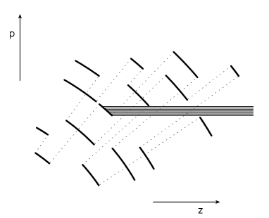
Figure 2: Photon escape chanels for $N=3$. The dotted lines indicate where dense shells got fragmented. The lines drawn parallel to the $z$ axis indicate photon escape chanels towards the observer.

3 Opaque fragments

3.1 Optical depth in fragmented wind

To calculate the optical depth in radial direction for the fragmented wind, consider an arbitrary radius $r$, infinitesimal radial increment $\delta r$, and an area element $A$ of arbitrary shape that is oriented perpendicular to the radial direction. $A$ shall be much larger than the average local fragment area. The radial optical depth increment is (note, $r=1$ at the atmospheric rim),

$$\delta\tau_{r}={\displaystyle\delta\!A_{b}\over\displaystyle A}={\displaystyle NA\,\delta r\over\displaystyle A(1-\epsilon)}\approx N\,\delta r,$$ (1)

where $\delta\!A_{b}$ is the area of opaque atomic absorbers in the volume $A\,\delta r$. From Eq. (1), the total radial optical depth between $\epsilon$ and 1 is $N$, in agreement with the foregoing section. We drop from now on $\epsilon$ in nonsingular expressions, still using equation signs, i.e. $\epsilon\rightarrow 0$ is assumed.

Figure 3: Basic geometry in the wind.

The observer shall be located at $z=\infty$ in standard $pz$ coordinates. Introducing the direction cosine $\mu={\bf r}\cdot{\bf z}$ with unity vectors ${\bf r}$ and ${\bf z}$, one has $v_{z}=\mu v_{r}$ and $\delta z=\delta r/\mu$, see Fig. 3. The optical depth increment for a photon propagating in $z$ direction is,

$$\delta\tau_{z}=N\,\delta z\,\mu=N\,\delta r.$$ (2)

The factor $\mu$ accounts for the reduction in optical depth caused by the foreshortening of the fragment area in photon propagation direction. Note that this is equivalent to an angle-dependent opacity

$$\chi=\mu N.$$ (3)

Another way to look at Eq. (2) is that, for a given pathway $\delta z$, $N\,\delta r$ is the average number of fragment hits (assuming a uniform fragment distribution), which is precisely the definition of the optical depth increment. This is elaborated upon in the appendix. The total optical depth, $\tau(r,\mu)$, from an X-ray emission site specified by coordinates $r$ and $\mu$ to the outer boundary of the atmosphere along the $p$ ray with $p=r\sqrt{1-\mu^{2}}$ is therefore simply the difference of the respective radii $r$ at these two locations,

$$\tau(r,\mu)=\begin{cases}N(1-r)&\text{if $\mu>0$},\\ N(1+r-2p)&\text{if $\mu<0$}.\end{cases}$$ (4)

We neglect obscuration due to the central region of radius $\epsilon$, which is easy to include in a numerical code but would cause lengthy case distinctions in the present equations.

The conclusion is that $\tau(r,\mu)$ is independent of $p=p(r,\mu)$ and therefore of $\mu$ if $\mu>0$, i.e. for the blue part of the line profile forming in gas that moves towards the observer. Therefore, the optical depth is the same for all photons that originate on the surface of a given front hemisphere. The reason is that $\tau$ is the expectation value of the number of fragment hits between the emission site and the outer boundary of the atmosphere. Since the spatial distribution of fragments depends neither on latitude nor azimuth, one can arrange them, on average, to spherical shells. The same number of shells, $N(1-r)$, is crossed by each $p$ ray that starts on the hemisphere with radius $r$. For $\mu<0$, on the other hand, i.e. the red part of the profile, the number of shells crossed is $N(r-p)$ on the back hemisphere, and $N(1-p)$ on the front hemisphere, giving in total $\tau(r,\mu<0)=N(1+r-2p)$ as in Eq. (4).

3.2 Optical depth in homogeneous wind

We compare the above expressions for $\tau$ with those in homogeneous wind. The fragments consist of atomic absorbers of cross section $\sigma_{0}$ that have number density $n_{0}/r^{2}$ in the homogeneous wind in which the fragments form ($v=v_{\infty}$; and we chose a reference radius $r_{0}=1$). The total optical depth of the homogeneous wind in radial direction is $t=\int_{\epsilon}^{1}\sigma_{0}n(r)dr$. In the limit $\epsilon\rightarrow 0$, $t=\sigma_{0}n_{0}/\epsilon$, using equation signs if errors of order $\epsilon$ are made. The optical depth increment in $z$ direction is $\delta\tau_{z}=\sigma_{0}n(r)\,\delta z=t\epsilon\delta z/r^{2}$. Note that for isotropic absorbers, no $\mu$ factor occurs here in contrast to Eq. (2). According to Fig. 3,

$$\delta\tau_{z}=t\epsilon{\displaystyle\delta\theta\over\displaystyle p},$$ (5)

where $\delta\theta=\delta z\sqrt{1-\mu^{2}}/r$ is the change in latitude over the pathway $\delta z$. With $p$ being constant, the $z$ integral is replaced by a $\theta$ integral, giving (e.g. MacFarlane et al. 1991)

$$\tau(r,\mu)={\displaystyle t\epsilon\over\displaystyle p}({\rm acos}\,\mu-{\rm asin}\,p),$$ (6)

independent of the sign of $\mu$.

3.3 Flat-topped profile from emitting sphere in an optically thin wind

Consider a spherical shell with outflow speed $v$ and uniform surface distribution of X-ray emitters. There shall be no absorption in the volume inside or outside the shell, and stellar occultation is neglected. The X-ray intensity measured by an observer at infinity is $I_{\nu}=dE_{\nu}/d\nu\,d\omega\,dt\,dA$, with the usual meaning of the symbols. Integrating over n $d\omega$ gives for the flux, $F_{\nu}\sim dE_{\nu}/d\nu$. Due to the Doppler effect, $\nu=\nu_{0}+\mu v/v_{\rm th}$, where $\nu_{0}$ is the rest frame frequency of the line and $v_{\rm th}$ the thermal speed. Hence $d\nu\sim d\mu$ and $d\nu/d\theta\sim\sin\theta$. The energy emitted at a given line frequency $\nu(\mu)$ is $dE_{\nu}\sim\eta\,dV=\eta\,dr\cdot rd\theta\cdot 2\pi r\sin\theta$. Therefore $F_{\nu}\sim dE_{\nu}/d\theta\cdot d\theta/d\nu\sim r^{2}dr\,\eta(r)$. Since any reference to $\mu$ (or $\theta$) has vanished, the line profile is flat-topped.

3.4 X-ray line profiles for opaque fragments

We turn to X-ray line formation in a dense wind with absorption. For constant radial wind speed $v(r)=v_{\infty}$, the surfaces of constant projected velocity $\mu v$ as seen by an observer at infinity are straight cones of opening angle ${\rm acos}\,\mu$. The emergent line profile is given by

$$F^{e}_{\mu}\sim\int_{\epsilon}^{x}dr\,r^{2}\,\eta(r)\,e^{-\tau(r,\mu)},$$ (7)

with $\tau(r,\mu)$ from Eqs. (4) or (6). Only $\tau$ depends on $\mu$, i.e. refers to the explicit cone considered. Since $\tau(r,\mu)$ from Eq. (4) is independent of $\mu$ for $\mu>0$, the blue part of the line profile from the fragmented wind remains flat-topped, despite absorption. This is not true for the homogeneous wind. All photons emitted from the surface of a given front hemisphere are diminished by the same optical depth (the fragment hit expectation value), hence the emission line profile stays flat-topped even after severe absorption. Note that in a wind with nonconstant outflow speed, the flat-topped profiles from individual emitting spheres of radius $r$ have different widths $[-v(r),+v(r)]$ in velocity space, hence the sum of individual line profiles is no longer a flat-topped profile.

We repeat the physical argument for flat-topped blueshifted parts of line profiles despite wind absorption: divide the X-ray emitting volume into spherical layers of infinitesimal thickness. If the wind would be optically thin, the line emission from each of these shells would show a flat-topped profile. Consider the front hemisphere towards the observer where the blueshifted component of the profile forms. Because the distribution of absorbing fragments obeys spherical symmetry, one can arrange them, on average, on spherical shells (with uniformly distributed holes). Therefore, all photons reaching the observer at infinity from a given radius $r$ in the front hemisphere encounter, on average, the same number of absorber fragments, i.e. experience the same optical depth. Hence, the blue part of the profile remains flat.

Figure 4 shows line profiles from the fragmented and, for comparison, from the homogeneous wind. The latter shows the well-known red-blue asymmetry, with a rather uniform decline from the blue to the red line wing (MacFarlane et al. 1991; Ignace 2001; Owocki & Cohen 2001). By contrast, the profile for the fragmented wind is almost a step function, namely flat-topped over the whole blueshifted part, and with steep decline to zero intensity on the redshifted part. We suggest that such a profile, after convolution with the detector response function, resembles the blueshifted yet symmetric emission line profiles observed from $\zeta$ Pup, see Fig. 3 in Cassinelli et al. (2001). By the same token, its blueshift is too large to be reconcilable with $\zeta$ Ori’s observed emission lines. For Chandra and XMM-Newton, the line center frequency can be measured with an accuracy of roughly 5 mÅ, which corresponds to $\delta v/v_{\infty}\approx 0.06$ at 1 keV, assuming $c/v_{\infty}=150$. This is almost one order of magnitude smaller than the blueshift $\delta v/v_{\infty}\approx 0.5$ in Fig. 4.

Figure 4: X-ray emission line profiles. Full: fragmented wind with opaque absorbers; dotted: homogeneous wind. Parameters are: $N=10$ dense fragments per radial ray; inner atmospheric radius $\epsilon=0.1$; termination radius $x=1$ for X-ray emission; radial optical depth $t=3$ of the homogeneous wind. The abscissa is in units of the projected, normalized wind speed, $\mu=v_{z}/v_{\infty}$.

As a conclusion from this section, observed X-ray line profiles of $\zeta$ Pup and $\zeta$ Ori are qualitatively different. Our model of a fragmented stellar wind can only explain the former.

4 Nonopaque fragments

4.1 Fragment optical depth

We drop now assumption (7), and account for the finite optical depth of fragments. The latter shall form close to the photosphere in a rather uniform process, and therefore contain roughly the same number of atoms. The radial optical depth of a fragment is the absorber area per fragment area, $\sigma_{0}n_{0}/Nr^{2}$ or $t\epsilon/Nr^{2}$. In the limit $1/N\equiv dr\rightarrow 0$ of infinitely many, optically thin fragments, the integral over $dr$ gives $t$, as must be. On the other hand, for a finite number $N$ of optically thick fragments, the expression for the total radial optical depth becomes,

$$t_{\rm f}=\int_{\epsilon}^{1}dr\,N\,\left[1-\exp\left({-t\epsilon\over Nr^{2}}\right)\right].$$ (8)

This is derived in Eq. (17) of the appendix, but is also intuitively clear: the integrand is the product of the hit expectation value of a fragment – which is the optical depth increment for opaque fragments, see Eq. (1) – times the transmission probability for nonopaque fragments. For a large number of optically thin fragments, $N\rightarrow\infty$, the exponential can be Taylor-series expanded to first order, giving again $t_{\rm f}=t$. In the opposite limit of opaque fragments, the exponential term is dropped, giving $t_{\rm f}=N$ as in Sect. 2.2. Turning to moderately optically thick fragments, we shift the lower integration bound in Eq. (8) to 0 and make a variable substitution $y=1/r$. Integrating by parts,

$$t_{\rm f}/N=1-e^{-a}+\sqrt{a\pi}\bigl{(}1-{\rm erf}\sqrt{a}\bigr{)},$$ (9)

where $a=t\epsilon/N$ and ${\rm erf}\,x=2\pi^{-1/2}\int_{0}^{x}e^{-t^{2}}dt$. The average optical depth per fragment is $t_{\rm f}/N=0.17$ for $a=0.01$ (optically thin fragments), is 0.46 for $a=0.1$, and is 0.91 for $a=1$ ($t_{\rm f}/N=1$ for opaque fragments).

Cassinelli & Olson (1979) and Hillier et al. (1993) estimate that the total radial optical depth of the wind of $\zeta$ Pup could reach 30 at 1 keV. Time-dependent hydrodynamical simulations of O star winds suggest that there are of order 10 dense shells. Assuming, then, $t=30$, $N=10$, and $\epsilon=0.1$, one has $t\epsilon/N=0.3$. Around this value of $t\epsilon/N$, the line profile shape starts to resemble the profile from opaque fragments, see Figs. 5 and 6. We must thus conclude that assumption (7) of opaque fragments is only applicable for rather dense winds.

4.2 X-ray lines profiles for nonopaque fragments

According to the above, the optical depth $\tau_{r\mu}$ of a single fragment located at radius $r$, with direction cosine $\mu$, is

$$\tau_{r\mu}={t\epsilon\over Nr^{2}\mu}$$ (10)

in $z$ direction. Here, $\mu$ accounts for the longer pathway through the fragment when seen under an angle $\theta$. The formal integral for the line profile shape becomes

$$F^{e}_{\mu} \sim\int_{\epsilon}^{x}dr\,r^{2}\,\eta(r)\,e^{-\tau(r,\mu)},$$

$$\tau(r,\mu) =\int_{r}^{1}dr^{\prime}\,N\,\left[1-\exp\left({-t\epsilon\over Nr^{\prime 2}\mu^{\prime}}\right)\right].$$ (11)

This cannot be solved analytically, but is easily evaluated numerically.

Figure 5: Normalized X-ray emission line profiles from winds with increasing optical depth (top: optically thin; bottom: very optically thick). Full lines show the fragmented wind model, dotted lines the homogeneous wind. Parameters are $N=10$, $\epsilon=0.1$, $x=1$, $\eta\sim r^{-4}$. The numbers at the top right give the total radial optical depth $t$ of the homogeneous wind, and the ratios of emergent to intrinsic X-ray flux.

Figure 5 shows X-ray line profiles at different values of the wind optical depth $t$. From Eq. (8), assumption (7) of opaque fragments holds if $t\epsilon/N\gtrsim 1$. In accordance with this, the line profile in the bottom panel of Fig. 5, at $t\epsilon/N=10$, resembles that for fully opaque fragments from Fig. 4. The same is essentially true for the second panel from bottom, at $t\epsilon/N=1$. At smaller $t$, however, the profiles for the fragmented and homogeneous wind become similar, as is seen in the two top panels of the figure.

At present it is not clear, which fraction of intrinsic X-rays become visible as emergent X-rays. For O stars, the latter typically amount to $10^{-7}\,L$, with bolometric luminosity $L$ (Sciortino et al. 1990). The wind kinetic energy, on the other hand, which is the ultimate reservoir for X-ray energy via thermalization of macroscopic flow energy into heat by shocks, comprises for $Lv_{\infty}/2c$ or $10^{-3}-10^{-2}\,L$ if the wind is close to the single-scattering limit, $L/c\approx\dot{M}v_{\infty}$, and if $v_{\infty}\lesssim c/100$. Therefore, there is a large potential margin between intrinsic and emergent X-rays. The models shown in Fig. 5 all lie within this margin.

4.3 Size of X-ray emitting region

Figure 6: Similar to Fig. 5, but with smaller X-ray emitting volume, $x=0.3$. Still $N=10$, $\epsilon=0.1$.

Hydrodynamic simulations show that shock-compressed, absorbing fragments significantly reexpand above $\approx 30\,R_{\ast}$ due to internal pressure, and the wind gradually becomes homogeneous again. On the other hand, X-ray emitting shocks (e.g. as caused by collisions of fast wind clouds with fragments) may only reach out to $10\,R_{\ast}$, suggesting $x=0.3$ in assumption (8).

Figure 6 shows line profiles for this value of $x$. The major differences when compared to Fig. 5 are: (i) the decline on the red part of the profile is more gradual now; (ii) the blue part of line profiles from the fragmented wind starts to become flat-topped at $t\epsilon/N\gtrsim 0.1$ already; (iii) for the homogeneous wind at $t\epsilon/N=1$, the ratio of emergent to intrinsic X-rays is very small, $4\times 10^{-14}$.

4.4 Natal fragment absorption

We assumed so far that X-rays originate from homogeneous emission within a sphere of radius $x$. Instead, X-ray emission may spatially coincide with the oriented, absorbing fragments. The line deshadowing instability is expected to form strong, X-ray emitting shocks that cool radiatively, leading to highly compressed fragments of cool, absorbing wind gas. If the radiative cooling zone is narrow, one can think of both X-ray emission and absorption occuring in the same, spherical segments. The shocks are of the braking type, i.e. are reverse shocks on the starward facing side of fragments. X-ray emitters on the front hemisphere, $\mu>0$, are then hidden behind their natal fragment, whereas emitters on the back hemisphere are not. To treat natal fragment absorption, we have to account for the finite optical depth of fragments, since else the whole blueshifted part of the line profile would turn black. For photons from the back hemisphere, we use $\tau(r,\mu)$ from Eq. (4.2) in the formal integral, however with $N\,dr$ replaced by $(N-1)\,dr$ because the natal shell is not hit. For photons emitted from the front hemisphere, $\tau(r,\mu)$ is replaced by $\tau(r,\mu)+\tau_{r\mu}$, with $\tau_{r\mu}$ the optical depth of the natal fragment from Eq. (10). In Eq. (4.2), $N\,dr\rightarrow(N-1)\,dr$ again, to avoid double counting the optical depth of the natal shell.

Figure 7 shows the resulting line profiles. Since $\tau_{r\mu}$ from Eq. (10) becomes infinite at $\mu=0$, the center of the profile from the optically thick, fragmented wind is black. This kind of double-peaked X-ray emission line profile is not observed. The resolution of the Chandra and XMM-Newton gratings is sufficiently high as to resolve such a profile shape.

We are drawn to conclude that either forward shocks exist of a strength similar to that of the reverse shocks, and prevent the drop to zero intensity; or that the assumption of spatial proximity of X-ray emitters and absorbers in 2-D, oriented fragments is too strong. The former alternative seems unlikely; the latter is rather plausible, given that both lateral motions (eddies) and a finite extent of radiative cooling zones could prevent emitters at $\mu\geq 0$ from being hidden behind their natal fragment. Therefore, a homogeneous distribution of X-ray emitters as in assumption (8) seems more appropriate than a strict coincidence of emitters and absorbers in 2-D, oriented fragments.

Figure 7: Similar to Fig. 5, but with natal fragment absorption included.

5 Summary

We consider X-ray emission line formation in a spherically symmetric stellar wind with constant radial outflow speed. X-rays are assumed to originate from hot gas within a sphere of radius $x$. Cool, absorbing wind gas resides in flat, highly overdense fragments that are oriented perpendicular to the radial flow direction. The fragments are thought to result from radial fragmentation of compressed gas shells that form due to the line deshadowing instability. The fragments have infinitesimal opening angle, a uniform spatial distribution, and partake in radial expansion. Our results are:

1. For opaque fragments, the blueshifted part of the line profile is flat-topped, even after strong absorption, whereas the redshifted part drops steeply to zero. The overall profile is therefore essentially flat-topped with a full width of $v_{\infty}$ and a blueshift of $v_{\infty}/2$. This is in stark contrast to the well-known gradual decline from the blue to the red line wing for a homogeneous wind. The line profiles from the fragmented wind could explain why observed X-ray line profiles from $\zeta$ Pup are strongly blueshifted, yet can be fitted by a Gaussian function.

2. A blueshift of $v_{\infty}/2$ is too large to be in accord with the (essentially) unshifted X-ray line profiles observed from $\zeta$ Ori and $\theta^{1}$ Ori C. We suggest that X-rays from these stars do not originate in instability-generated wind shocks, but in colliding wind shocks or processes involving magnetic fields.

3. The assumption of opaque fragments is applicable if $t\epsilon/N\gtrsim 1$ ($t$ the radial optical depth of the homogeneous wind between radii $\epsilon$ and 1; $N$ the number of fragments along radial rays), as could be the case for dense O star winds like $\zeta$ Pup’s. On the other hand, with decreasing optical depth of nonopaque fragments, line profiles become similar to those from a homogeneous wind.

4. X-ray absorption in natal fragments leads to zero flux at line center. This kind of double-peaked profile is not observed, which suggests that lateral motions and a finite extent of radiative cooling zones prevents a strict spatial coincidence of X-ray emitters and absorbers in 2-D, oriented fragments.

Quantitative modelling of X-ray emission line profiles of $\zeta$ Pup accounting for an accelerating wind and instrumental broadening will be subject of a forthcoming paper.

Appendix A A Poisson ring

We take here a different view at X-ray absorption in a wind with oriented absorbers, using Poisson statistics. The two objectives of this appendix are (i) to make explicit the connection of fragment hits and optical depth, and (ii) to obtain an expression for X-ray transmission through nonopaque absorbers. We assume $N=1$ throughout, and generalize to $N>1$ at the end of the appendix. In the fragmented wind, consider a ring with radius $p$ centered on the $z$ axis at latitude $\theta$. The probability that a photon propagating at impact parameter $p$ hits an absorber fragment along the ring is $\delta w_{z}=\delta r$ within a pathway $\delta z$. Decrease $\delta z$ until each fragment that is hit along the ring within this $\delta z$ fully covers the interval $[\theta,\theta+\delta\theta]$. Next, divide the ring into $N_{\phi}$ azimuthal segments of width $\delta\phi=\delta\theta$. Since the fragment hit probability $\delta w_{z}$ in each of these segments is small and the number $N_{\phi}$ of segments (or “trials”) is large, the requirements for a Poisson distribution are met. The single parameter of the latter is the expectation value, $\lambda$, here of fragment hits,

$$\lambda=N_{\phi}\,\delta w_{z}={\displaystyle 2\pi\mu p\over\displaystyle{1-\mu^{2}}},$$ (12)

using $\delta r=\mu p\,\delta\phi/({1-\mu^{2}})$. To give an example, consider the ring with $p=1/2$ and $\theta=45^{\circ}$ ($\mu=1/\sqrt{2}$). On average, $\lambda=\pi\sqrt{2}\approx 4.44$ fragments are hit along this ring, in a pathway $\delta z$. The independence of the number of hits from $N_{\phi}$ is easily understood: if $N_{\phi}$ is doubled, $\delta\phi$, $\delta\theta$, $\delta z$, and $\delta w_{z}$ drop by a factor of two, leaving $\lambda$ unchanged.

The probability $\pi(k)$ that $k$ fragments are hit along the full ring is,

$$\pi(k)={\displaystyle\lambda^{k}\over\displaystyle k!}e^{-\lambda},\qquad k=0,1,2,\ldots$$ (13)

Photons at different $\phi$ have different absorption histories, but for simplicity we assume that the whole ring is illuminated by an average intensity $\langle I^{\rm i}\rangle$. Summing the intensity $I^{\rm o}$ after absorption within $\delta z$ over all segments $\delta\phi$,

$$I_{1}^{\rm o}+I_{2}^{\rm o}+\ldots I_{N_{\phi}}^{\rm o}=N_{\phi}\langle I^{\rm o}\rangle=\hfill$$

$$\qquad=\pi(0)\;\langle I^{\rm i}\rangle\;N_{\phi}$$

$$\qquad+\pi(1)\;\langle I^{\rm i}\rangle\;\bigl{(}N_{\phi}-1+e^{-\tau_{r\mu}}\bigr{)}$$

$$\qquad+\pi(2)\;\langle I^{\rm i}\rangle\;\bigl{(}N_{\phi}-2+2e^{-\tau_{r\mu}}\bigr{)}$$ (14)

$$\qquad+\ldots$$

$$\qquad+\pi(N_{\phi})\;\langle I^{\rm i}\rangle\;\;N_{\phi}\,e^{-\tau_{r\mu}},$$

where $\tau_{r\mu}$ is the fragment optical depth at radius $r$ in direction ${\rm acos}\,\mu$. Inserting (13) and using the binomial formula for $k\ll N_{\phi}$ (as can be safely assumed for a Poisson distribution), it follows that

$$\langle I^{\rm o}\rangle=\langle I^{\rm i}\rangle\,e^{-\lambda}\sum_{k=0}^{\infty}{\displaystyle\lambda^{k}\over\displaystyle k!}\left(\displaystyle 1-{1-e^{-\tau_{r\mu}}\over\displaystyle N_{\phi}}\right)^{k}.$$ (15)

The sum is the power series expansion of the exponential,

$$\langle I^{\rm o}\rangle=\langle I^{\rm i}\rangle\;e^{-\lambda}e^{\lambda\left(1-{1-e^{-\tau_{r\mu}}\over N_{\phi}}\right)}=\langle I^{\rm i}\rangle\;e^{-\delta w_{z}\left(1-e^{-\tau_{r\mu}}\right)}.$$ (16)

The case $N>1$ is treated by making $N$ copies of the atmosphere, and eliminating $N-1$ fragments along the radial rays in each of the copies. The $N$ copies with one remaining fragment per radial ray are arranged like pearls on a string, and photons pass subsequently through each of them. Hence, for $N>1$, $\delta w_{z}$ in Eq. (16) has to be replaced by $N\,\delta w_{z}$, giving as optical depth increment along $\delta z$,

$$\delta\tau_{z}=N\left(1-e^{-\tau_{r\mu}}\right)\delta r.$$ (17)

For opaque fragments, this reduces to Eq. (2) of the main text. According to Eq. (17), the partial transparency of the fragments leads to a reduction of their effective opacity by a factor $1-\exp(-\tau_{r\mu})$, i.e. we obtain

$$\chi=\mu N\left(1-e^{-\tau_{r\mu}}\right)$$ (18)

in replacement of Eq. (3).

References

- (1)
- (2) Cassinelli, J. P., & Olson, G. L. 1979, ApJ, 229, 304
- (3) Cassinelli, J. P., Miller, N. A., Waldron, W. L., MacFarlane, J. J., & Cohen, D. H. 2001, ApJ, 554, L55
- (4) Hillier, D. J., Kudritzki, R. P., Pauldrach, A. W., et al. 1993, A&A, 276, 117
- (5) Ignace, R. 2001, ApJ, 549, L119
- (6) Kahn, S. M., Leutenegger, M. A., Cottam, J., et al. 2001, A&A, 365, L312
- (7) Lucy, L. B. 1982, ApJ, 255, 278
- (8) MacFarlane, J. J., Cassinelli, J. P., Welsh, B. Y., et al. 1991, ApJ, 380, 564
- (9) Mewe, R., Raassen, A., Cassinelli, J. P., et al. 2003, A&A, 398, 203
- (10) Miller, N. A., Cassinelli, J. P., Waldron, W. L., MacFarlane, J. J., & Cohen, D. H. 2002, ApJ, 577, 951
- (11) Owocki, S. P., & Cohen, D. H. 2001, ApJ, 559, 1108
- (12) Owocki, S. P., Castor, J. I., & Rybicki, G. B. 1988, ApJ, 335, 914
- (13) Rybicki, G. B., Owocki, S. P., & Castor, J. I. 1990, ApJ, 349, 274
- (14) Schulz, N. S., Canizares, C. R., Huenemoerder, D., & Lee, J.,C. 2000, ApJ, 545, L135
- (15) Sciortino, S., Vaiana, G. S., Harnden, F. R., et al. 1990, ApJ, 361, 621
- (16) Waldron, W. L., & Cassinelli, J. P. 2001, ApJ, 548, L45
- (17)