Ultra-High Energy Cosmic Rays in a Structured and Magnetized Universe

Abstract

We simulate propagation of cosmic ray nucleons above $10^{19}\,$eV in scenarios where both the source distribution and magnetic fields within about 50 Mpc from us are obtained from an unconstrained large scale structure simulation. We find that consistency of predicted sky distributions with current data above $4\times 10^{19}\,$eV requires magnetic fields of $\simeq 0.1\mu$G in our immediate environment, and a nearby source density of $\sim 10^{-4}-10^{-3}\,{\rm Mpc}^{-3}$. Radio galaxies could provide the required sources, but only if both high and low-luminosity radio galaxies are very efficient cosmic ray accelerators. Moreover, at $\simeq 10^{19}\,$eV an additional isotropic flux component, presumably of cosmological origin, should dominate over the local flux component by about a factor three in order to explain the observed isotropy. This argues against the scenario in which local astrophysical sources of cosmic rays above $\simeq 10^{19}\,$eV reside in strongly magnetized ($B\simeq 0.1\mu$G) and structured intergalactic medium. Finally we discuss how future large scale full-sky detectors such as the Pierre Auger project will allow to put much more stringent constraints on source and magnetic field distributions.

I Introduction

Over the last few years the detection of several giant air showers, either through ground based detectors haverah ; agasa or fluorescence telescopes  fe ; hires , has confirmed the arrival of ultra high energy cosmic-rays (UHECRs) with energies up to a few hundred EeV (1 EeV $\equiv 10^{18}\,$eV). Their existence poses a serious challenge and is currently subject of much theoretical research as well as experimental efforts (for recent reviews see reviews ; bs-rev ; school ).

The problems encountered in trying to explain UHECRs in terms of “bottom-up” acceleration mechanisms have been well-documented in a number of studies (e.g., Refs. hillas-araa ; ssb ; norman ). In summary, apart from the specific energy draining interactions in the source the maximal UHECR energy is limited by the product of the accelerator size and the strength of the magnetic field. According to this criterion it turns out that it is very hard to accelerate protons and heavy nuclei up to the observed energies, even for the most powerful astrophysical objects such as radio galaxies and active galactic nuclei.

In addition, nucleons above $\simeq 70\,$EeV suffer heavy energy losses due to photo-pion production on the cosmic microwave background (CMB) — the Greisen-Zatsepin-Kuzmin (GZK) effect gzk — which limits the distance to possible sources to less than $\simeq 100\,$Mpc stecker . Heavy nuclei at these energies are photo-disintegrated in the CMB within a few Mpc heavy . Unless the sources are strongly clustered in our local cosmic environment, a drop, often called the “GZK cut-off” in the spectrum above $\simeq 70\,$EeV is therefore expected bbo , even if the injection spectra extend to much higher energies. However, the existence of the latter is not established yet from the observations mbo . In fact, whereas a cut-off seems consistent with the few events above $10^{20}\,$eV recorded by the fluorescence detector HiRes hires , it is not compatible with the 8 events (also above $10^{20}\,$eV) measured by the AGASA ground array agasa . The solution of this problem may have to await the completion of the Pierre Auger project auger which will combine the two complementary detection techniques adopted by the aforementioned experiments.

Adding to the problem, there are no obvious astronomical counterparts to the detected UHECR events within $\simeq 100\,$Mpc of the Earth elb-som ; ssb . At the same time, no significant large-scale anisotropy has been observed in UHECR arrival directions above $\simeq 10^{18}\,$eV, whereas there are strong hints for small-scale clustering: The AGASA experiment has observed five doublets and one triplet within $2.5^{\circ}$ out of a total of 57 events detected above 40 EeV agasa . When combined with three other ground array experiments, these numbers increase to at least eight doublets and two triplets within $4^{\circ}$ uchihori . This clustering has a chance probability of less than $1\%$ in the case of an isotropic distribution.

Independent of the specific UHECR production mechanism, there are currently two possible explanations of the experimental findings described above: The first assumes very weak intergalactic magnetic fields capable of deflecting UHECRs only up to a few degrees, or neutral primaries. In this case the apparent isotropy would indicate that many sources contribute to the observed flux and most of these sources would be at cosmological distances because the local source distribution is in general too anisotropic to be consistent with the observed UHECR isotropy. This would also explain the absence of nearby counterparts and a subset of especially powerful sources would explain the small-scale clustering tt . Indeed, it has been argued that UHECR arrival directions correlate with the positions of BL Lacertae objects, suggesting these as sources accelerating protons bllac , although there seems to be disagreement about this in the literature bllac1 . Furthermore, some of these objects may be too far away to be consistent with the GZK effect, which would require new physics such as Lorentz symmetry violations jlm . In contrast, correlations with compact radio quasars have not been found c_quasar . If correlations with astrophysical objects are confirmed, this would strongly suggest small deflection or neutral primary particles. Whatever the sources are in this scenario, for small deflection one can in principle constrain the characteristics of the magnetic fields along the line of sight and the source properties by analysing arrival times, directions, and energies of observed small-scale multi-plets sl . Also, in the small deflection scenario the experimental confirmation of a GZK cutoff is expected.

However, the assumption of weak intergalactic magnetic fields seems at odds with several observations kronberg . Most remarkable are the detections of Faraday rotation measures which seem to indicate field strengths at the $\mu$G level within the inner region ($\sim$ central Mpc) of galaxy clusters  bo_review . In addition, the recent mounting evidence for diffuse radio-synchrotron emission in numerous galaxy clusters gife00 and in a few cases of filaments kkgv89 ; bagchietal02 , seems to suggest the presence of magnetic fields as strong as 0.1-1.0$\mu$G at the relatively low density outskirts of collapsed cosmological structures. In fact, extragalactic magnetic fields (EGMF) as strong as $\simeq 1\mu G$ in sheets and filaments of the large scale galaxy distribution, such as in our Local Supercluster, are compatible with existing upper limits on Faraday rotation bo_review ; ryu ; blasi . It is also possible that fossil cocoons of former radio galaxies, so called radio ghosts, contribute to the isotropization of UHECR arrival directions mte . Thus, relatively strong magnetic fields seem to be ubiquitous in intergalactic space, although their theoretical understanding is still limited bt_review .

Such observational evidence motivates a second, more realistic scenario, which takes into account the existence of strong ($B\sim 0.1-1\,\mu$G) intergalactic magnetic fields correlated with the large scale structure. In this case magnetic deflection of charged primaries would be considerable even at the highest energies and the observed UHECR flux could be dominated by relatively few sources within about 100 Mpc. Here, large scale isotropy could be explained by considerable angular deflection leading to diffusion up to almost the highest energies and the small scale clustering could be due to magnetic lensing hmrs . The locations of clusters of events of different energies would in this case coincide with the crossing points of the caustics for these energies where fluxes are enhanced.

In the present paper we take this second point of view and investigate in some detail the effects of propagation of UHECRs, assumed to be dominantly nucleons, in a magnetized large scale structure matter distribution computed according to a numerical cosmological simulation.

Early investigations of this scenario have been carried out in Refs. slb ; ils ; lsb ; sse ; is , assuming that sources and magnetic fields follow a pancake profile of scale height $\simeq 3\,$Mpc and scale length $\simeq 20\,$Mpc, the magnetic field having a power law spectrum at length scales below $\simeq 1\,$Mpc. UHECR propagation was computed through a numerical code that accounts for magnetically induced deflections and all relevant energy losses slb ; lsb ; ils . The cases of a single source slb ; ils , as well as continuous lsb and discrete source distributions  is have been investigated. The above studies led to the result that the multi-pole moments and autocorrelation functions of the arrival directions best fit the AGASA data for a number $\sim$10 sources in the Local Supercluster, assumed to emit continuously, and a maximal field strength of $\simeq 0.3\mu\,$G is .

Ideally, however, it would be desirable to study the propagation of UHECRs based on distributions of both potential sources and observed magnetic field properties. However, up to now, only catalogs of candidate sources have been available. Magnetic fields, on the other hand, have been approximated in a number of fashions: as negligible sommers , as uniform ynts , or as organized in spatial cells with a given coherence length and a strength depending as a power law on the local density tanco .

In the present paper we attempt to go beyond some of the above limitations by computing for the first time the propagation of the UHECRs in a magnetized cosmological environment computed through numerical simulations. We carry out a fully cosmological simulation of large scale structure formation which, in addition to dark matter and baryonic gas, follows the evolution of a passive magnetic field. This approach is motivated by the fact that $\mu$G magnetic fields are mostly negligible for the purpose of the dynamics of the large scale cosmic flows (hence their passive character). In addition, and basically for the same reason, the structure of magnetic fields on scales of interest for UHECR propagation ($\sim$ 100 kpc) is mostly determined by the hydrodynamic flow. This is confirmed by the fact that in these simulations, the magnetic field looses memory of its initial conditions, soon after the formation of structures begins. Finally, the statistical properties of cosmological structure in the universe are rather homogeneous. Therefore, the simulated matter structure and magnetic field distributions should provide a realistic scenario for studying the statistical properties of UHECR source distributions and propagation in a cosmic environment. In the present study we assume the sources to follow the baryon density. Furthermore, the observer is supposed to be in regions of the simulated matter distribution which contain structures of the same size and baryonic gas temperature as our local neighborhood. This should provide a suitable environment to simulate the arrival of UHECRs from extragalactic distances and the effects of local magnetic fields of various strengths.

In the future such studies can be further improved by computing constrained simulations that reproduce in detail the observed matter distribution of the local universe. Such a simulation has been used for the case of radio ghosts in Ref. mte where, however, the magnetic fields were not followed but were rather assumed to scale with the gas density. Constrained simulations including magnetic fields are relevant for predicting quantitative features such as location of clustered events, phases of anisotropies etc. and will be used in a following study. We point out, however, that for the reasons given above, effects of the magnetic field and source distributions in the local universe should essentially be captured by the present approach at least up to “cosmic variance”. The latter represents variations due to different source and observer locations and will be estimated in our simulations.

We also restrict ourselves to UHECR nucleons, and we neglect the Galactic contribution to the deflection of UHECR nucleons since typical proton deflection angles in galactic magnetic fields of several $\mu$G are $\lesssim 10^{\circ}$ above $4\times 10^{19}\,$eV medina , and thus in general are small compared to extra-galactic deflection in the scenarios studied in the present paper.

The simulation is described in more detail in the next section. There we also describe the general features of our method and define the statistical quantities used for comparison with the data. In Sect. 3 we present results and we conclude in Sect. 4.

II Motivation and Outline of the Numerical Model

II.1 Magnetic Deflection

Contrary to the case of electrons, for charged hadrons deflection is more important than synchrotron loss in the EGMF. To get an impression of typical deflection angles one can characterize the EGMF by its r.m.s. strength $B$ and a coherence length $l_{c}$. If we neglect energy loss processes for the moment, then the r.m.s. deflection angle over a distance $r\gtrsim l_{c}$ in such a field is $\theta(E,r)\simeq(2rl_{c}/9)^{1/2}/r_{L}$ wm , where the Larmor radius of a particle of charge $Ze$ and energy $E$ is $r_{L}\simeq E/(ZeB)$. In numbers this reads

$$\theta(E,r) \simeq 0.8^{\circ}\,Z\left(\frac{E}{10^{20}\,{\rm eV}}\right)^{-1}\left(\frac{r}{10\,{\rm Mpc}}\right)^{1/2}$$ (1)

$$\hskip 28.45274pt\times\left(\frac{l_{c}}{1\,{\rm Mpc}}\right)^{1/2}\left(\frac{B}{10^{-9}\,{\rm G}}\right)\,,$$

for $r\gtrsim l_{c}$. This expression makes it immediately obvious why a magnetized Local Supercluster with fields of fractions of micro Gauss prevents a direct assignment of sources in the arrival directions of observed UHECRs; the deflection expected is many tens of degrees even at the highest energies. This goes along with a time delay

$$\tau(E,r) \simeq r\theta(E,d)^{2}/4$$

$$\simeq 1.5\times 10^{3}\,Z^{2}\left(\frac{E}{10^{20}\,{\rm eV}}\right)^{-2}\left(\frac{r}{10\,{\rm Mpc}}\right)^{2}$$

$$\hskip 28.45274pt\times\left(\frac{l_{c}}{\rm Mpc}\right)\left(\frac{B}{10^{-9}\,{\rm G}}\right)^{2}\,{\rm yr}\,,$$

which may be millions of years. A source visible in UHECRs today could therefore be optically invisible since many models involving, for example, active galaxies as UHECR accelerators, predict variability on much shorter time scales.

II.2 Numerical Simulation of the Large Scale Structure

The formation and evolution of the large scale structure is computed by means of an Eulerian, grid based Total-Variation-Diminishing hydro+N-body code rokc93 . We adopt a canonical, flat $\Lambda$CDM cosmological model with a total mass density $\Omega_{m}=0.3$ and a vacuum energy density $\Omega_{\Lambda}=1-\Omega_{m}=0.7$. We assume a normalized Hubble constant $h_{67}\equiv H_{0}/67$ km s^-1 Mpc^-1 = 1 and a baryonic mass density, $\Omega_{b}=0.04$. The simulation is started at redshift $z\simeq 60$ with initial density perturbations generated as a Gaussian random field and characterized by a power spectrum with a spectral index $n_{s}=1$ and “cluster-normalization” $\sigma_{8}=0.9$.

We adopt a computational box size of $50\,h_{67}^{-1}\,$Mpc. In this box the dark matter component is described by 256³ particles whereas the gas component is evolved on a comoving grid of 512³ zones. Thus each numerical cell measures about $100\,h_{67}^{-1}\,$kpc (comoving) and each dark matter particle corresponds to $2\times 10^{9}\,h_{67}^{-1}\,M_{\odot}$. Besides the box and dark matter particle sizes the cosmological simulation is the same as that presented in Ref. miniati .

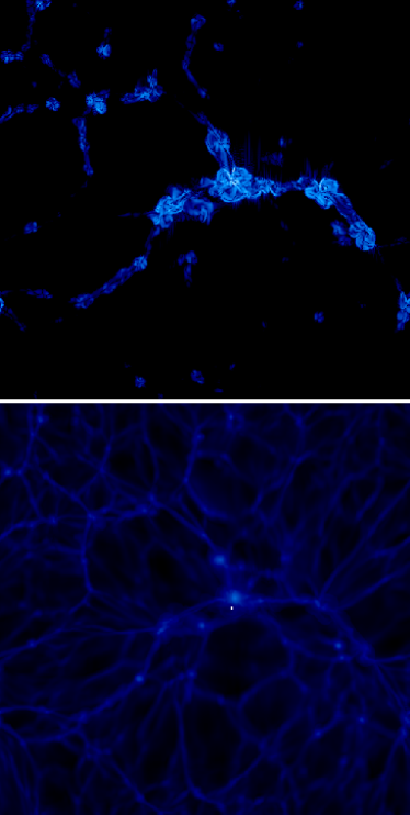
Figure 1: Log-scale two-dimensional cut through magnetic pressure (top) and baryon density (bottom). The image is $50\,h_{67}^{-1}\,$Mpc on each side and $100\,h_{67}^{-1}\,$kpc deep. The small white dot in the bottom panel indicates the location of the observer. For visualization purposes we adopt a dynamic range of 3 and 6 orders of magnitude for the magnetic pressure and baryon density, respectively.

The magnetic field is followed as a passive quantity, that is magnetic forces are neglected. This is consistent with the strength of observed magnetic fields in most diffuse extragalactic environments. Basically we solve the induction equation with the velocity field provided by the simulated flow kcor97 and the initial magnetic field seeds generated by the Biermann battery mechanism. However, as already pointed out, the initial conditions are not important as the topological properties of the magnetic field are determined by the subsequent evolution of the large scale flow. This is responsible for its amplification through gas compression and shear flows. Thus, at the end of the simulation, the relative strength of the magnetic field in different regions is determined by the hydrodynamic properties of the flow. While the simulation outcome regarding the relative magnetic field strength and topology distribution are obviously retained, the overall normalization is chosen in order to reproduce the fields of several micro Gauss observed in the regions of largest density, namely galaxy cluster cores. Fig. 1 illustrates an example of the simulated magnetic pressure (top) and baryonic density (bottom) distributions. The figure shows two-dimensional cuts corresponding to a depth of $100\,h_{67}^{-1}\,$kpc. The color images are in log scale and, for visualization purposes, span a dynamic range of 3 and 6 orders of magnitude for magnetic pressure and baryonic density respectively. The magnetic field is particularly strong in both postshock regions and inside relatively large structures where it has been compressed and stretched. Apparently, its distribution is less concentrated than the baryonic density, resembling in this respect that of the thermal pressure (not shown).

II.3 Simulated UHECR Experiments

To simulate the propagation and arrival of UHECRs in the computational box we need to choose: (a) the location of the observer and (b) the source distribution. As anticipated in the introduction, the location of the observer is identified as a region whose general features in terms of scale, mass and temperature, resemble those of the local universe. That means a small group of galaxies characterized by a gas temperature of order of a fraction of a keV. There are several such structures in a $50\,h_{67}^{-1}\,$Mpc box such as the one employed here. In the neighborhood of the one we selected as the observer location, we also find a larger group of galaxies with temperature of a few keV. In order to orient the simulation box with respect to the observed sky, the latter object, located at a distance of $\sim$ 34 Mpc, is arbitrarily associated with the Virgo cluster. This reference frame allows us to define a celestial system of coordinates $(\alpha,\delta)$ which describes the arrival direction of events recorded by our virtual observer. It will be useful in the next section where the arrival direction probability distribution is constructed. The above setting is sufficient for the current purpose of investigating the effects on the propagation of UHECRs of realistic, topologically structured magnetic fields of various strengths.

We then chose randomly a certain total number $N_{s}$ of sources in the box, corresponding to an average source density $8\times 10^{-6}h_{67}^{3}\,N_{s}\,{\rm Mpc}^{-3}$, with probability proportional to the local baryon density. In order to avoid introducing too many free parameters, we further assume that all sources roughly emit the same power law spectrum of CRs extending up to $\simeq 10^{21}\,$eV, with roughly equal total power. We also assume that neither total power nor the power law spectral index change significantly on the time scale of UHECR propagation. This can be up to a few Giga years for the magnetic fields considered here. Injected power and spectral index are then treated as parameters which can be fit to reproduce the observed spectrum, as will be seen below.

For each such configuration many nucleon trajectories originating from the sources were computed numerically by solving the equation of motion for the Lorentz force and checking for pion production every fraction of a Mpc according to the total interaction rate with the CMB and, in case of an interaction, by randomly selecting the secondary energies according to the differential cross section. Pair production by protons is treated as a continuous energy loss process.

A detection event was registered and its arrival directions and energies recorded each time the trajectory of the propagating particle crossed a sphere of radius 1 Mpc around the observer. For each configuration this was done until 5000 events where registered. For more details on this method see Refs. slb ; lsb ; ils .

II.4 Data Processing

For each realization of sources and observer, these events were used to construct arrival direction probability distributions, taking into account the solid-angle dependent exposure function for the respective experiment and folding over the angular resolution.

For the exposure function $\omega(\delta)$ we use the parameterization of Ref. sommers which depends only on declination $\delta$,

$$\omega(\delta) \propto \cos(a_{0})\cos(\delta)\sin(\alpha_{m})+\alpha_{m}\sin(a_{0})\sin(\delta)\,,$$

$$\mbox{where}\hskip 14.22636pt\alpha_{m}=\left\{\begin{array}[]{ll}\ 0&\mbox{if $\xi>1$}\\ \ \pi&\mbox{if $\xi<-1$}\\ \ \cos^{-1}(\xi)&\mbox{otherwise}\end{array}\right.\,,$$

$$\mbox{with}\hskip 14.22636pt\xi\equiv\frac{\cos(\theta_{m})-\sin(a_{0})\sin(\delta)}{\cos(a_{0})\cos(\delta)}\,.$$

For the AGASA experiment $a_{0}=-35^{\circ}$, $\theta_{m}=60^{\circ}$, and the angular resolution $2.4^{\circ}$ are used. For a full-sky Pierre Auger type experiment we add the exposures for the Southern Auger site with $a_{0}=-35^{\circ}$ and a putative similar Northern site with $a_{0}=39^{\circ}$, and $\theta_{m}=60^{\circ}$ in both cases, with an assumed angular resolution of $\simeq 1^{\circ}$.

From the distributions obtained in this way typically 1000 mock data sets consisting of $N$ observed events were selected randomly. For each such mock data set or for the real data set we then obtained estimators for the spherical harmonic coefficients $C(l)$ and the autocorrelation function $N(\theta)$. The estimator for $C(l)$ is defined as

$$C(l)=\frac{1}{2l+1}\frac{1}{{\cal N}^{2}}\sum_{m=-l}^{l}\left(\sum_{i=1}^{N}\frac{1}{\omega_{i}}Y_{lm}(u^{i})\right)^{2}\,,$$ (7)

where $\omega_{i}$ is the total experimental exposure at arrival direction $u^{i}$, ${\cal N}=\sum_{i=1}^{N}1/\omega_{i}$ is the sum of the weights $1/\omega_{i}$, and $Y_{lm}(u^{i})$ is the real-valued spherical harmonics function taken at direction $u^{i}$. The estimator for $N(\theta)$ is defined as

$$N(\theta)=\frac{C}{S(\theta)}\sum_{j\neq i}\left\{\begin{array}[]{ll}1&\mbox{if $\theta_{ij}$ is in same bin as $\theta$}\\ 0&\mbox{otherwise}\end{array}\right\}\,,$$ (8)

and $S(\theta)$ is the solid angle size of the corresponding bin. In Eq. (8) the normalization factor $C=\Omega_{e}/(N(N-1))$, with $\Omega_{e}$ denoting the solid angle of the sky region where the experiment has non-vanishing exposure, is chosen such that an isotropic distribution corresponds to $N(\theta)=1$.

The different mock data sets in the various realizations yield the statistical distributions of $C(l)$ and $N(\theta)$. One defines the average over all mock data sets and realizations as well as two errors. The smaller error (shown to the left of the average in the figures below) is the statistical error, i.e. the fluctuations due to the finite number $N$ of observed events, averaged over all realizations. The larger error (shown to the right of the average in the figures below) is the “total error”, i.e. the statistical error plus the cosmic variance. Thus, the latter includes the fluctuations due to finite number of events and the variation between different realizations of observer and source positions.

Given a set of observed and simulated events, after extracting some useful statistical quantities $S_{i}$, namely $C_{l}$ and $N(\theta)$ defined above, we define

$$\chi_{n}\equiv\sum_{i}\left(\frac{S_{i,{\rm data}}-\overline{S}_{i,{\rm simu}}}{\Delta S_{i,{\rm simu}}}\right)^{n}\,,$$ (9)

where $S_{i,{\rm data}}$ refers to $S_{i}$ obtained from the real data, and $\overline{S}_{i,{\rm simu}}$ and $\Delta S_{i,{\rm simu}}$ are the average and standard deviations of the simulated data sets. This measure of deviation from the average prediction can be used to obtain an overall likelihood for the consistency of a given theoretical model with an observed data set by counting the fraction of simulated data sets with $\chi_{n}$ larger than the one for the real data.

III Results

In the following we compare the results obtained for the simulated UHECR propagation experiments described above with the observational results. In accord with what was outlined in the previous section, the comparison is based on the statistical properties of the simulated and observed events, expressed in terms of the angular power spectrum and the autocorrelation function of the UHECR arrival distributions. A summary of the simulations run is contained in Tab. 1. There, for comparison, simulations 2 and 5 were performed for an observer situated in a small void with weak ambient magnetic fields.

Table 1: List of UHECR propagation simulations. The columns contain the simulation number, the number of sources in the simulation box of $(50\,{\rm Mpc}\,h_{67}^{-}1)^{3}$, the magnetic field strength at the observer location, the best fit power law index in the injection spectrum $E^{-\alpha}$, and the overall likelihoods of fits to the AGASA data above $4\times 10^{19}\,$eV for the multi-poles Eq. (7) with $l\leq 10$ and the auto-correlation Eq. (8) for $\theta\leq 10^{\circ}$, respectively. The likelihoods are computed for $n=4$ in Eq. (9) which leads to reasonable discriminative power.

#	$N_{s}$	$B_{\rm obs}/$G	$\alpha$	${\cal L}_{l\leq 10}$	${\cal L}_{\theta\leq 10^{\circ}}$
1	100	$1.3\times 10^{-7}$	2.4	0.13	0.63
2	100	$8.2\times 10^{-12}$	2.7	0.098	0.15
3	10	$1.3\times 10^{-7}$	2.4	0.12	0.69
4	10	$2.7\times 10^{-7}$	2.4	0.071	0.15
5	10	$8.2\times 10^{-12}$	2.7	0.011	0.037
6	1	$1.3\times 10^{-7}$	2.8	0.074	0.62

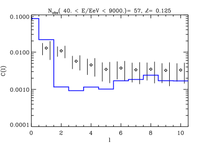
Figure 2: The angular power spectrum $C(l)$ as a function of multi-pole $l$, obtained for the AGASA exposure function, see text, for $N=57$ events observed above 40 EeV, sampled from 12 simulated configurations of scenario 1 in Tab. 1. The diamonds indicate the realization averages, and the left and right error bars represent the statistical and total (including cosmic variance due to different realizations) error, respectively, see text for explanations. The histogram represents the AGASA data. The overall likelihood significance is $\simeq 0.13$ for $n=4$ and $l\leq 10$ in Eq. (9).

Figure 3: As Fig. 2, but for the angular correlation function $N(\theta)$ as a function of angular distance $\theta$, using a bin size of $\Delta\theta=1^{\circ}$. Note that an isotropic distribution would correspond to $N(\theta)=1$. The overall likelihood significance is $\simeq 0.63$ for $n=4$ and $\theta\leq 10^{\circ}$ in Eq. (9). It is not significantly different for somewhat larger bin sizes $\Delta\theta\simeq 2^{\circ}$.

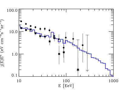
Figure 4: Predicted spectrum observable by AGASA for the scenario 1 in Tab. 1, for which multipoles and auto-correlations were shown in Figs. 2 and 3, averaged over 12 realizations, as compared to the AGASA (dots) and HiRes-I (stars) data.

We find that as long as the observer is surrounded by magnetic fields of about $0.1\mu$G, $N_{s}\gtrsim 10$ nearby sources, i.e. sources within the simulation box, are necessary to reproduce multi-poles and autocorrelations marginally consistent with present data, limited, we emphasize, to the Northern hemisphere only. However, consistency of large scale multi-poles is somewhat worse than for the spatially more extended EGMF assumed in previous work is . In Figs. 2 and 3 we show as an example the results for the case of $N_{s}=100$ nearby sources, scenario 1 in Tab. 1, corresponding to a source density of $8\times 10^{-4}h_{67}^{3}\,\,{\rm Mpc}^{-3}$. The overall likelihood for $n=4$ in Eq. (9) is $\simeq 0.13$ and $\simeq 0.63$ for the multi-poles and autocorrelations shown, respectively. Also Fig. 4 shows that, for UHECR sources characterized by a proton injection spectrum roughly as $\propto E^{-2.4}$ and extending up to $\simeq 10^{21}\,$eV, the observed spectrum at sub-GZK energies is well reproduced. In addition, above GZK energies the spectral slope is predicted to be somewhere between the AGASA and HiRes observations, see Fig. 4. Normalizing to the observed flux results in a UHECR power of $5\times 10^{41}{\rm erg}\,{\rm s}^{-1}$ per source to be continuously emitted above $10^{19}\,$eV.

The situation for $N_{s}=10$ nearby sources does not lead to significantly different likelihoods, see scenarios 3 and 4 in Tab. 1. However, the case of just one source is clearly disfavored in terms of the multi-poles, see scenario 6 in Tab. 1. This confirms similar findings in earlier work ils .

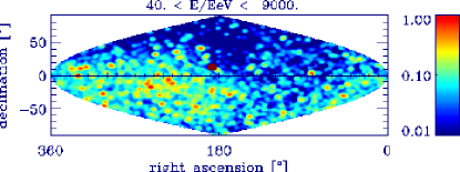
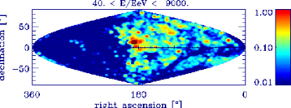
Figure 5: Illustration of the influence of magnetic fields surrounding the observer on UHECR arrival direction distributions above 40 EeV in terrestrial coordinates. The upper panel is for scenario 1 (observer surrounded by relatively strong magnetic fields), and the lower panel for scenario 2 (observer surrounded by negligible magnetic fields) from Tab. 1, averaged over all 12 and 10 realizations of 5000 trajectories each, respectively, thus corresponding to an effective number of sources of $\sim 1000$. The color scale represents the integral flux per solid angle. The pixel size is $1^{\circ}$ and the image has been convolved to an angular resolution of $2.4^{\circ}$ corresponding to the approximate AGASA angular resolution. The filled sphere represents the position of the Virgo-like cluster.

If the observer is in a region of EGMF strength much smaller than $\simeq 0.1\mu$G, as in scenario 2 of Tab. 1, for $N_{s}\gtrsim 100$ nearby sources the predicted UHECR sky distribution reflects the highly structured large scale galaxy distribution, smeared out only by the fields surrounding the sources. This becomes obvious from Fig. 5 which shows that UHECR arrival directions are much less isotropic in this case than if the observer is immersed in fields $B\simeq 0.1\mu$G.

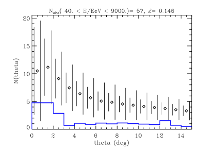
Figure 6: Similar to Fig. 3, but for an observer in a much lower field region, $\simeq 8.2\times 10^{-12}\,$G. This corresponds to scenario 2 in Tab. 1. The overall likelihood significance is $\simeq 0.15$ for $n=4$ and $\theta\leq 10^{\circ}$ in Eq. (9).

Nevertheless, the overall likelihood significance for multi-poles up to $l=10$ is $\simeq 0.1$, and thus not significantly worse than for the strong observer field case of Fig. 2. Therefore, the number of events observed by AGASA above $40\,$EeV is insufficient to distinguish this low observer field case from the strong observer field case based on anisotropy alone. However, as can be seen from Fig. 6, the low observer field case results in auto-correlations at angles $\theta\gtrsim 3^{\circ}$ much larger than observed by AGASA. This is because strong magnetic fields at the observer position cause enough UHECR diffusion that their large-scale auto-correlations are significantly suppressed, as in Fig. 3. However, for fields considerably larger than $0.1\mu$G the auto-correlations tend to become too strong again, see scenario 4 in Tab. 1, probably due to increased magnetic lensing.

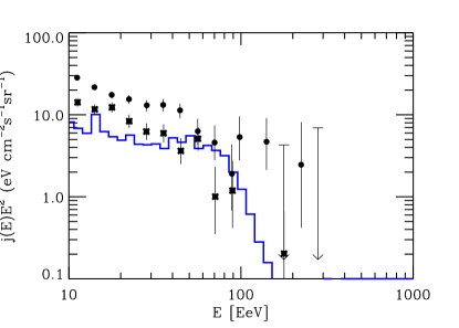
Figure 7: The unnormalized energy spectrum observed at Earth resulting from a $E^{-2.4}$ isotropic proton flux injected at a sphere of 40 Mpc radius around the observer for scenario 1 from Tab. 1, averaged over solid angle and $10^{4}$ computed trajectories. In contrast to the spectrum of the local component shown in Fig. 4, there is a clear tendency that this cosmological component can fit the flux neither at the highest nor at the lowest energies.

We also find that sources outside our Local Supercluster do not contribute significantly to the observable flux if the observer is immersed in magnetic fields above about $0.1\mu$G and if the sources reside in magnetized clusters and super-clusters: For particles above the GZK cutoff this is because sources outside the Local Supercluster are beyond the GZK distance. On the other hand, sub-GZK particles are mainly confined in their local magnetized environment and thus exhibit a much higher local over-density than their sources. Further, the suppressed flux of low energy particles leaving their environment is largely kept away from the observer if he is surrounded by significant magnetic fields is . Both effects can be understood qualitatively by matching the flux $j(E)$ in the unmagnetized region with the diffusive flux $-D(E){\bf\nabla}n(E,{\bf r})$ in terms of the diffusion coefficient $D(E)$ and the density $n(E,{\bf r})$ of particles of energy $E$ which shows that the density gradient always points to the source. More quantitatively, the shape of the large-distance component is demonstrated in Fig. 7 which shows the observable flux resulting from an $E^{-2.4}$ spectrum injected isotropically at a sphere with a radius of 40 Mpc around the observer. Note that despite the smaller energy losses the sub-GZK particles arriving from outside the Local Supercluster are likely to have a spectrum even more strongly suppressed than in Fig. 7 at low energies due to their containment in the source region. A significant contribution from sources at cosmological distances to sub-GZK energies thus requires that neither these sources nor the observer are immersed in too strong magnetic fields and/or an injection spectrum considerably steeper than $E^{-2.4}$ to compensate for the systematic suppression of flux of lower energy particles.

The confidence levels that can be obtained with this method for specific models of our local magnetic and UHECR source neighborhood will greatly increase with the increase of data from future experiments. Full sky coverage alone will play an important role in this context as many scenarios predict large dipoles for the UHECR distribution. This is the case for basically all scenarios considered here, as demonstrated in Fig. 8. Whereas current northern hemisphere data are consistent with scenarios with $N_{s}\gtrsim 10$ nearby sources at the $\simeq 1.5\,$sigma level if the observer is surrounded by relatively strong fields $B\sim 0.1\,\mu$G, a comparable or larger exposure in the southern hemisphere would be sufficient in these cases to find a dipole at several sigma confidence level, as demonstrated in Fig. 8.

Figure 8: Same as Fig. 2, but for comparison of the model predictions with an isotropic distribution [horizontal line, $C_{l}\simeq(4\pi N)^{-1}$, see Eq. (7)] for the full-sky detector à la Auger discussed in the text, for $N=150$ events observed above 40 EeV.

Finally, the distributions of events down to $10^{19}\,$eV also contain important information. Fig. 9 shows the multi-poles predicted by our standard scenario 1 in Tab. 1 that full-sky experiment would observe for 1500 events detected above $10^{19}\,$eV. This corresponds to twice the number of currently observed AGASA events and thus approximately reflects the current exposure. A corresponding figure for the AGASA detector alone would look similar. It is obvious that there is significant anisotropy even at $l\simeq 10$, inconsistent with current AGASA observations. On the other hand, cosmic variance becomes more important at these lower energies, and a possible significant contribution from large-distance sources cannot be excluded if their magnetization is not too high, as discussed above. It is easy to see from Eq. (7) that if a fraction $f_{a}$ of $N$ events observed stems from an anisotropic, local contribution, whereas the fraction $1-f_{a}$ is cosmological and completely isotropic, then

$$C_{l}\simeq C_{l,i}\left((1-f_{a})^{2}+\frac{C_{l,a}}{C_{l,i}}f_{a}^{2}\right)\,,$$ (10)

where $C_{l,i}=(4\pi N)^{-1}$ and $C_{l,a}$ are the expectation values of $C_{l}$ for the isotropic and the anisotropic distribution, respectively. Therefore, at $\simeq 10^{19}\,$eV an isotropic cosmological flux about a factor 3 higher than the anisotropic flux originating within $\simeq 50\,$Mpc would be needed to explain the isotropy observed by AGASA. For charged primaries this implies steep injection spectra and/or weak magnetic fields around observer and sources, as explained above. Without going into a more detailed analysis we remark that this will also require to decrease the flux contribution from nearby sources shown in Fig. 4 at the low energy end. As a consequence, the best fit injection spectrum for the local component will be slightly harder than the power law indices shown in Tab. 1. This is consistent with what is expected from shock acceleration theory rel_shock .

Figure 9: Same as Fig. 8, but for $N=1500$ events observed above 10 EeV.

IV Conclusions

In the present work we performed UHECR propagation simulations based on the distributions of magnetic field and baryon density obtained from a simulation of large scale structure formation. The magnetic field was simulated as a passive quantity and normalized at simulation end in agreement with published measurements of Faraday rotation measures for groups and clusters of galaxies bo_review . We considered finite numbers of discrete UHECR sources with equal total power and injection spectrum. Their positions were randomly selected with probability proportional to the baryon density. The observer was chosen within small groups of galaxies characterized by gas temperatures around a fraction of a keV, typical for our local environment. One chosen observer was found in a relatively high field region with $B\simeq 0.1\mu$G. For comparison, we also chose an observer situated in a small void, where the surrounding field is $B\simeq 10^{-11}\,$G. We found that good fits to the AGASA data above $4\times 10^{19}\,$eV in the Northern hemisphere are only obtained for $N_{s}\gtrsim 10$ sources and for observers surrounded by $\simeq 0.1\mu$G fields. Otherwise the predicted arrival direction distribution is either too anisotropic or produces too large auto-correlations at angles larger than a few degrees. The best fit case occurs for $N_{s}\simeq 100$, significantly higher than in previous work is due to the more localized and more strongly structured magnetic fields considered here.

For the required local source number density and continuous power per source we find $n_{\rm source}\gtrsim 10^{-4}-10^{-3}\,h_{67}^{3}{\rm Mpc}^{-3}$, and $Q_{\rm source}\lesssim 5\times 10^{41}{\rm erg}\,{\rm s}^{-1}$ respectively, the latter within about one order of magnitude uncertainty to both sides. This corresponds to an average UHECR emissivity of $q_{\rm UHECR}=n_{\rm source}\,Q_{\rm source}\sim 10^{38}{\rm erg\,Mpc^{-3}\,s^{-1}}$ also with an uncertainty of roughly one order of magnitude, not larger, since it is fixed by the observed UHECR flux.

Possible sources marginally consistent with these energy requirements are radio galaxies. Their present energy release of $q_{\rm rg}\sim 5\times 10^{39}\,{\rm erg\,s^{-1}\,Mpc^{-3}}\,(f_{\rm power}/10)$ ebkw97 is roughly what is required in order to produce a sufficient flux of UHECR, assuming that the injection power law is flat ($\propto E^{-2}$) rb93 ; rsb93 . The parameter $f_{\rm power}$ describes the ratio of the total power of the radio galaxy to the equipartition estimate based on its radio luminosity, and it enters the used radio luminosity-jet-power relation of ebkw97 . We expect $f_{\rm power}\sim 10$ within an order of magnitude. In the estimate of the radio galaxy power the observed radio luminosity function dp90 was integrated only for sources with a 2.7 GHz luminosity of more than $L_{\rm min}=2\times 10^{22}\,{\rm Watt\,Hz^{-1}}$, since they correspond to a luminosity of $10^{43}\,{\rm erg\,s^{-1}}\,(f_{\rm power}/10)$. This would provide the required UHECR luminosity per source of $Q_{\rm source}\sim 5\times 10^{41}{\rm erg}\,{\rm s}^{-1}(f_{\rm power}\,f_{\rm UHECR}/0.5)$, using the optimistic assumption of rb93 ; rsb93 that $f_{\rm UHECR}=3-10\%$ of the radio galaxy power is converted into UHECRs. The implied number density of these radio galaxies is $n_{\rm source}\sim 10^{-4}\,{\rm Mpc^{-3}}$ and, therefore, is only marginally consistent with the required $n_{\rm source}\sim 10^{-4}-10^{-3}\,h_{67}^{3}{\rm Mpc}^{-3}$. Since the number density increases strongly with decreasing $L_{\rm min}$ this requirement can possibly be fulfilled by allowing for a larger number of less powerful UHECR sources. This implies that basically every radio galaxy has to be an efficient UHECR source, not only the most powerful ones. Since many of the weaker radio galaxies do not exhibit a hot spot, which is assumed to be the UHECR acceleration site in the scenario of rb93 ; rsb93 , their efficiency in producing UHECR might be largely reduced. This is a potential serious problem for this scenario, since lowering $f_{\rm UHECR}$ by several orders of magnitude can not be fully compensated by assuming a higher radio galaxy jet-power, because $f_{\rm power}>100$ does not seem to be consistent with observations of radio galaxies 1992A&A…265….9F .

To conclude, radio galaxies can be the sources of UHECRs if even weak radio galaxies are efficient particle accelerators to the highest energies, otherwise they have serious problems to reproduce the smooth UHECR arrival direction distribution.

We also found that consistency with the isotropy observed by AGASA down to $10^{19}\,$eV requires the existence of an isotropic component with a flux about a factor 3 larger than the local component. This isotropic component would presumably be of cosmological origin and thus would not contribute significantly above $4\times 10^{19}\,$eV due to the GZK effect, consistent with the fact that at these energies we find local scenarios consistent with all data. The resulting best fit injection spectrum for the local component is $E^{-(2.2-2.4)}$. In contrast, for the charged primaries of the cosmological component to dominate around $10^{19}\,$eV steep injection spectra and/or weak magnetic fields around observer and sources would be required. These two conflicting requirements provide a strong argument against the hypothesis of local astrophysical sources of UHECRs above $\simeq 10^{19}\,$eV in a strongly magnetized and structured intergalactic medium.

Finally, we have also demonstrated that already a modest increase in data together with full-sky coverage will allow to put considerably stronger constraints on UHECR source and magnetic field scenarios than presently possible. In particular, our local scenarios predict the emergence of significant dipoles and quadrupoles above $4\times 10^{19}\,$eV.

Modeling our cosmic neighborhood and simulating UHECR propagation in this environment will therefore become more and more important in the coming years. This will also have to include the effects of the Galactic magnetic field and an extension to a possible heavy component of nuclei. For first steps in this direction see, e.g. Refs. mte ; ames , and Ref. bils , respectively.

References

- (1) See, e.g., M. A. Lawrence, R. J. O. Reid, and A. A. Watson, J. Phys. G Nucl. Part. Phys. 17 (1991) 733, and references therein; see also http://ast.leeds.ac.uk/haverah/hav-home.html.
- (2) M. Takeda et al., Phys. Rev. Lett. 81 (1998) 1163; Astrophys. J. 522 (1999) 225; Hayashida et al., e-print astro-ph/0008102; see also http ://www-akeno.icrr.u-tokyo.ac.jp/AGASA/.
- (3) D. J. Bird et al., Phys. Rev. Lett. 71 (1993) 3401; Astrophys. J. 424 (1994) 491; ibid. 441 (1995) 144.
- (4) T. Abu-Zayyad et al. (HiRes collaboration), e-print astro-ph/0208243; e-print astro-ph/0208301.
- (5) for recent reviews see J. W. Cronin, Rev. Mod. Phys. 71 (1999) S165; M. Nagano, A. A. Watson, Rev. Mod. Phys. 72 (2000) 689; A. V. Olinto, Phys. Rept. 333-334 (2000) 329; X. Bertou, M. Boratav, and A. Letessier-Selvon, Int. J. Mod. Phys. A15 (2000) 2181; G. Sigl, Science 291 (2001) 73.
- (6) P. Bhattacharjee and G. Sigl, Phys. Rept. 327 (2000) 109; L. Anchordoqui, T. Paul, S. Reucroft, and J. Swain, Int. J. Mod. Phys. A18 (2003) 2229.
- (7) “Physics and Astrophysics of Ultra High Energy Cosmic Rays”, Lecture Notes in Physics, vol. 576 (Springer Verlag, 2001), eds. M. Lemoine, G. Sigl.
- (8) A. M. Hillas, Ann. Rev. Astron. Astrophys. 22 (1984) 425.
- (9) G. Sigl, D. N. Schramm, and P. Bhattacharjee, Astropart. Phys. 2 (1994) 401.
- (10) C. A. Norman, D. B. Melrose, and A. Achterberg, Astrophys. J. 454 (1995) 60.
- (11) K. Greisen, Phys. Rev. Lett. 16 (1966) 748; G. T. Zatsepin and V. A. Kuzmin, Pis’ma Zh. Eksp. Teor. Fiz. 4 (1966) 114 [JETP. Lett. 4 (1966) 78].
- (12) F. W. Stecker, Phys. Rev. Lett. 21 (1968) 1016.
- (13) J. L. Puget, F. W. Stecker, and J. H. Bredekamp, Astrophys. J. 205 (1976) 638; L. N. Epele and E. Roulet, Phys. Rev. Lett. 81 (1998) 3295; J. High Energy Phys. 9810 (1998) 009; F. W. Stecker, Phys. Rev. Lett. 81 (1998) 3296; F. W. Stecker and M. H. Salamon, Astrophys. J. 512 (1999) 521.
- (14) see, e.g., M. Blanton, P. Blasi, and A. V. Olinto, Astropart. Phys. 15 (2001) 275.
- (15) for a discussion see, e.g., D. De Marco, P. Blasi, and A. V. Olinto., e-print astro-ph/0301497.
- (16) J. W. Cronin, Nucl. Phys. B (Proc. Suppl.) 28B (1992) 213; The Pierre Auger Observatory Design Report (ed. 2), March 1997; see also http://www.auger.org.
- (17) J. W. Elbert, and P. Sommers, Astrophys. J. 441 (1995) 151.
- (18) Y. Uchihori, M. Nagano, M. Takeda, M. Teshima, J. Lloyd-Evans, and A. A. Watson, Astropart. Phys. 13 (2000) 151.
- (19) P. G. Tinyakov and I. I. Tkachev, Pisma Zh. Eksp. Teor. Fiz. 74 (2001) 3 [JETP Lett. 74 (2001) 1].
- (20) P. G. Tinyakov and I. I. Tkachev, JETP Lett. 74 (2001) 445; D. S. Gorbunov, P. G. Tinyakov, I. I. Tkachev, and S. V. Troitsky, Astrophys. J. 577 (2002) L93.
- (21) N. W. Evans, F. Ferrer, and S. Sarkar, Phys. Rev. D 67 (2003) 103005; P. G. Tinyakov and I. I. Tkachev, e-print astro-ph/0301336.
- (22) G. Sigl, D. F. Torres, L. A. Anchordoqui, and G. E. Romero, Phys. Rev. D 63 (2001) 081302.
- (23) see, e. g., T. Jacobson, S. Liberati, and D. Mattingly, e-print hep-ph/0209264, and references therein.
- (24) G. Sigl and M. Lemoine, Astropart. Phys. 9 (1998) 65.
- (25) for a recent review see P. P. Kronberg, Physics Today 55, December 2002, p. 40.
- (26) P. P. Kronberg, Reports of Progress in Physics 58 (1994) 325; J. P. Vallée, Fundamentals of Cosmic Physics, Vol. 19 (1997) 1; T. E. Clarke, P. P. Kronberg, and H. Böhringer, Astrophys. J. Lett. 547 (2001) L111; J.-L. Han and R. Wielebinski, CHJA&A 2 (2002) 293 [e-print astro-ph/0209090].
- (27) G. Giovannini, and L. Feretti, New Astronomy 5 (2000) 335.
- (28) K.-T. Kim, P. P. Kronberg, G. Giovannini, and T. Venturi, Nature 341 (1989) 720
- (29) J. Bagchi, T. Enßlin, F. Miniati, C. S. Stalin, M. Singh, S. Raychaudhury, and N. B. Humeshkar New Astronomy 7 (2002) 249
- (30) D. Ryu, H. Kang, and P. L. Biermann, Astron. Astrophys. 335 (1998) 19.
- (31) P. Blasi, S. Burles, and A. V. Olinto, Astrophys. J. 514 (1999) L79.
- (32) G. Medina-Tanco and T. A. Enßlin, Astropart. Phys. 16 (2001) 47
- (33) for a review see, e.g., D. Grasso and H. Rubinstein, Phys. Rept. 348 (2001) 163.
- (34) see, e.g., D. Harari, S. Mollerach, E. Roulet, F. Sanchez, JHEP 0203 (2002) 045.
- (35) G. Sigl, M. Lemoine, and P. Biermann, Astropart. Phys. 10 (1999) 141.
- (36) C. Isola, M. Lemoine, and G. Sigl, Phys. Rev. D 65 (2002) 023004.
- (37) M. Lemoine, G. Sigl, and P. Biermann, e-print astro-ph/9903124.
- (38) T. Stanev, D. Seckel, and R. Engel, e-print astro-ph/0108338; see also T. Stanev, R. Engel, A. Mucke, R. J. Protheroe, and J. P. Rachen, Phys. Rev. D 62 (2000) 093005.
- (39) C. Isola and G. Sigl, Phys. Rev. D 66 (2002) 083002.
- (40) P. Sommers, Astropart. Phys. 14 (2001) 271.
- (41) H. Yoshiguchi, S. Nagataki, S. Tsubaki, and K. Sato, Astrophys. J. 586 (2003) 1211.
- (42) G. Medina Tanco, “Cosmic magnetic fields from the perspective of ultra-high-energy cosmic rays propagation”, Lect. Notes Phys. 576 (2001) 155.
- (43) G. Medina-Tanco, E. M. De Gouveia Dal Pino, and J. E. Horvath, e-print astro-ph/9707041.
- (44) E. Waxman and J. Miralda-Escudé: Astrophys. J.472 (1996) L89.
- (45) D. Ryu, J. P. Ostriker, H. Kang, and R. Cen, Astrophys. J. 414 (1993) 1
- (46) F. Miniati, Mon. Not. R.A.S. 337 (2002) 199
- (47) R. M. Kulsrud, R. Cen, J. P. Ostriker, and D. Ryu, Astrophys. J., 480 (1997) 481
- (48) J. G. Kirk, A. W. Guthmann, Y. A. Gallant, and A. Achterberg, Astrophys. J., 542 (2000) 235
- (49) T. A. Enßlin, P. L. Biermann, P. P. Kronberg, and X.-P. Wu, Astrophys. J.477 (1997) 560.
- (50) J. P. Rachen and P. L. Biermann, Astron. Astrophys. 272 (1993) 161.
- (51) J. P. Rachen, T. Stanev, and P. L. Biermann, Astron. Astrophys. 273 (1993) 377.
- (52) J. S. Dunlop and J. A. Peacock, Mon. Not. R.A.S. 247 (1990) 19
- (53) L. Feretti, G. C. Perola, and R. Fanti, Astron. Astrophys. 265 (1992) 9.
- (54) J. Alvarez-Muñiz, R. Engel, and T. Stanev, Astrophys. J. 572 (2001) 185.
- (55) G. Bertone, C. Isola, M. Lemoine, and G. Sigl, Phys. Rev. D 66 (2002) 103003.