Automated Determination of Stellar Parameters from Simulated Dispersed Images for DIVA

We have assessed how well stellar parameters ($T_{\rm eff}$, $\log g$ and [M/H]) can be retrieved from low-resolution dispersed images to be obtained by the DIVA satellite. Although DIVA is primarily an all-sky astrometric mission, it will also obtain spectrophotometric information for about 13 million stars (operational limiting magnitude $V\simeq 13.5$ mag). Constructional studies foresee a grating system yielding a dispersion of $\simeq$ 200nm/mm on the focal plane (first spectral order). For astrometric reasons there will be no cross dispersion which results in the overlapping of the first to third diffraction orders. The one-dimensional, position related intensity function is called a dispi (DISPersed Intensity). We simulated dispis from synthetic spectra taken from Lejeune et al. (1997) and Lejeune et al. (1998) but for a limited range of metallicites, i.e. our results are for [M/H] in the range $-$0.3 to 1 dex. We show that there is no need to deconvolve these low resolution signals in order to obtain basic stellar parameters. Using neural network methods and by including simulated data of DIVA’s UV telescope, we can determine $T_{\rm eff}$ to an average accuracy of about 2 % for dispis  from stars with 2000 K $\leq$ $T_{\rm eff}$ $\leq$ 20000 K and visual magnitudes of $V=13$ mag (end of mission data). $\log g$ can be determined for all temperatures with an accuracy better than 0.25 dex for magnitudes brighter than $V=12$ mag. For low temperature stars with 2000 K $\leq$ $T_{\rm eff}$ $\leq$ 5000 K and for metallicities in the range $-$0.3 to +1 dex a determination of [M/H] is possible (to better than 0.2 dex) for these magnitudes. For higher temperatures, the metallicity signatures are exceedingly weak at dispi resolutions so that the determination of [M/H] is there not possible. Additionally we examined the effects of extinction $E(B-V)$ on dispis and found that it can be determined to better than 0.07 mag for magnitudes brighter than $V=14$ mag if the UV information is included.

1 Introduction

The DIVA satellite was proposed in 1996 by a German consortium of astronomical institutes (Bastian et al. 1996, Röser et al. 1997) and is currently foreseen for launch in 2006. DIVA will measure the positions, brightnesses and proper motions of some 35 million stars. The scientific goal is to study the Milky Way and to improve the calibration of stellar properties and parameters. This mission follows up on the HIPPARCOS satellite which measured parallaxes for 100 000 stars. For about 20 000 of these stars, the accuracy in parallax was better than 10%. With the DIVA satellite this number of stars will be increased by at least a factor of 25 (Röser 1999).

DIVA will perform an all-sky survey with a limiting visual magnitude of $V\simeq 15.5$ mag. Note that every observed star will be measured about 120 times in the course of the mission. The stated magnitude limits refer to the combined images of all single measurements. The measurements include the precise determination of positions, trigonometric parallaxes, proper motions, colours and magnitudes. For about 13 million stars, spectrophotometric data will also be obtained down to a visual magnitude of $V\simeq 13.5$. An additional UV telescope will perform photometry in two spectral ranges adjacent to the Balmer jump.

Figure 1: Wavelength versus position on the spectroscopic CCD (SC) for the first, second and third order. The zeroth order which is made up of undispersed (white) light would lie at about pixel position 122, but is not shown.

The DIVA survey represents a large scale and deep astrometric and photometric survey of the local part in our Galaxy. The importance of these data to modern astrophysics will be significant, with applications ranging from stellar structure and evolution to cosmological aspects. Examples are a precise determination of the luminosity function in the solar neighbourhood, a better understanding of the structure and formation of our galaxy, the estimation of the amount of dark matter as well as a better calibration of the cosmological distance ladder (Röser 1999).

After the mission the photometric and spectrophotometric images will be used to obtain the brightness, the colour and the dispis  for the stars. The dispis will allow to derive the astrophysically relevant parameters $T_{\rm eff}$, $\log g$, [M/H] and $E(B-V)$.

Especially the derivation of $\log g$ is of importance for objects too distant to result in an accurate parallax. With these objects in mind, we have carried out the present study. We will demonstrate that the essential parameters of the stars can be retrieved with a reasonable level of accuracy from the dispis alone. We will show that astrophysical parameters can be well derived down to the survey limit, perhaps even adequately for stars 1 to 2 magnitudes fainter. There are good scientific arguments to reach fainter in selected fields, see e.g. Salim et al. (2002).

2 DIVA DISPIS

2.1 The concept of a DISPI

Figure 2: Transmission curves for the first, second and third grating orders, plus the quantum efficiency. The order’s curves have been scaled down by a factor of 0.6 to better represent data from the real grating.

The DIVA satellite is not only unique in its applications and abilities but also in the way it records spectra. DIVA will use a grating system yielding a dispersion of $\simeq$ 200nm/mm on the focal plane with a total efficiency of about 60%. For astrometric and other reasons, the resulting (spectral) orders of the grating are not separated. Thus “classical” spectrophotometry will not be obtained. Instead, the detector will record a pixel related intensity function for each star, in which all orders (and thus wavelengths) overlap. Such a one-dimensional position-coded intensity distribution is called dispi (DISPersed Intensity). Fig. 1 shows the position-coded wavelength of the grating’s orders. One can see that the resolution of the second and third orders increases by factors of two and three relative to the first order one, respectively. In the cross-dispersion direction, there are physical pixels while in the direction of dispersion there will be on-chip binning, resulting in “effective pixels”. One such effective pixel corresponds to about 11.6 nm in the first order.

The maximum transmission of the first order is at about 750 nm (see Fig. 2), while that of the second and third orders are at about 380 and 250 nm respectively (see also Scholz 1998, Scholz 2000).

2.2 Dealing with DISPIs

Given the nature of the dispis, a classical spectrophotometric analysis – like line and continuum fitting – to derive astrophysical parameters is cumbersome. We will show that by training Artificial Neural Networks (ANNs) on simulated dispis, we can readily access this information without any further pre-processing of the signal. Using dispis from calibration stars, i.e. stars with known physical and apparent properties, we would initially build up a standard set of dispi data. The automated classification technique as developed will then use this library. The calibration could be iteratively improved using dispis and their parametrization results obtained during the mission. Note that in these simulations, we did not use absolute fluxes as they will be available from the mission (see below). In this work, only the shape of a dispi and its line features were used for tests to determine basic stellar parameters.

Typical dispis can be seen in Fig. 3 and Fig. 4 for a cool and a hot star, respectively. One can see that the first, second and third orders contribute different amounts to the total light in a dispi for different temperatures. The first order’s transmission maximum is at about 700 nm while the second and third orders contribute mostly at shorter wavelengths. Thus, for the cooler star, the second order contributes less to the dispi in the case of the bluer, hotter star. The third order’s contribution becomes negligible for low temperatures. Note that the “continuum” of a dispi is mainly defined by the first and partly by the second order. For a hot star, spectral line features are essentially only visible in the second and third orders due to their two- and threefold higher resolution. Only for strong molecular bands in very cool stars are features resolved in the first order.

Table 1: The signal-to-noise ratio (S/N) for single measured dispis with different temperatures and visual magnitudes as measured from the 10 central pixels around effective pixel position 60 in the direction of dispersion. The innermost 13 TDI-rows of the two-dimensional SC image were summed up to build the dispi (see Sect. 4). The stated temperature is the central value for each sample (sample names are given in parentheses, see Table 2). The S/N for temperatures in the range of 6000 K $\leq$ $T_{\rm eff}$ $\leq$ 10000 K is almost the same for a given magnitude.

V[mag]	S/N
$T_{\rm eff}$= 3000 K ($L_{1}$)
8	122
9	77
10	47
11	28
12	16
$T_{\rm eff}$= 5000 K ($L_{2}$)
8	91
9	56
10	34
11	20
12	11
$T_{\rm eff}$= 9000 K ($L_{3}$,$M_{1}$,$M_{2}$)
8	82
9	50
10	30
11	17
12	9
$T_{\rm eff}$= 15000 K ($H_{1}$)
8	95
9	59
10	36
11	21
12	12
$T_{\rm eff}$= 30000 K ($H_{2}$)
8	118
9	74
10	46
11	28
12	16

The signal-to-noise ratio of a single dispi as measured from the 10 central pixels around effective pixel position 60 is shown for different visual magnitudes and temperatures in Table 1.

Figure 3: Input spectrum (top) and simulated DIVA dispi (bottom) for a star with $T_{\rm eff}$=4500 K, $\log g$= 4 and solar metallicity (no noise added). Top: the model spectrum sampled in steps of 4 nm, which matches roughly the resolution of the third order of the DIVA dispersed image, shows spectral structure of which the TiO band is marked. Bottom: DIVA dispi showing total counts (in arbitrary units) detected along the effective pixels in the extracted DIVA dispersed information. The TiO feature of the input spectrum (top) can be recognized in the contributions to the first and second orders.

Figure 4: Input spectrum (top) and simulated DIVA dispi (bottom) for a star with $T_{\rm eff}$= 9500 K, $\log g$= 4, solar metallicity (without noise, as in Fig. 3). Here the $H_{\alpha}$, $H_{\beta}$ and $H_{\gamma}$ features are marked in the model spectrum as well as in the resulting dispi. For such a star, the third order starts to contribute to the signal.

3 Artificial Neural Networks

Neural networks have proven useful in a number of scientific disciplines for interpolating multidimensional data, and thus providing a nonlinear mapping between an input domain (in this case the dispis) and an output domain (the stellar parameters). For an overview of Artifical Neural Networks (ANNs) and their application in astronomy for stellar classification see, for example, Bailer-Jones (2002). The software used in this work is that of Bailer-Jones (1998).

A network consists of an input layer, one or two hidden layers and an output layer. Each layer is made up of several nodes. All the nodes in one layer are connected to all the nodes in the preceding and/or following layers. These connections have adaptable “weights”, so that each node performs a weighted sum of all its inputs and passes this sum through a nonlinear transfer function. That weighted sum is then passed on to the next layer. Before the network can be used for parametrisation, it needs to be trained, meaning the weights have to be set to their appropriate values to perform the desired mapping. In this process, dispis together with known stellar parameters as target values are presented to the network. From these data, the optimum weights are determined by iteratively adjusting the weights between the layers to minimize an output error, i.e. the discrepancy between the targets and the network outputs. This is performed by a multidimensional numerical minimization, in this case with the conjugate gradients method. When this minimization converges, the weights are fixed and the network can be used in its “application” phase: now, only the dispi input flux vector is presented and the network’s outputs produce the stellar parameters of these dispis. Since we used only the central 51 effective pixels of the dispis (range 30 to 80, see Fig. 3 and 4), the input layer of the network was always made up of the same number of nodes, i.e. 51. We found that the performance was best when using two hidden layers, each containing 7 nodes. More nodes did not improve the result significantly but increased the training time considerably. With four output parameters this network then contains $51\cdot 7+7\cdot 7+7\cdot 4=434$ weights (plus 18 bias weights).

Since we wanted to classify dispis solely based on their shapes, the absolute flux information was removed by area-normalizing each dispi, i.e. each flux bin of a given dispi was divided by the total number of counts in that dispi. Given the non-uniform distribution of the training data over $T_{\rm eff}$, we classified dispis in terms of log $T_{\rm eff}$ instead of $T_{\rm eff}$.

Note that, in our tests, we have not included distance information as it eventually might be done using DIVA parallaxes, since the present goal was to test the retrieval of stellar parameters from dispis only.

The parametrization errors given below are the average (over some set of dispis) errors for each parameter, i.e.

$$A=\frac{1}{N}\cdot\sum_{p=1}^{N}\left|C(p)-T(p)\right|$$ (1)

where $p$ denotes the $p^{\rm th}$ dispi and $T$ is the target (or “true”) value for this parameter. Since the network’s function approximation can depend on the initial settings of the weights, it is sometimes recommended to use a “committee” of several networks with identical topologies but different initializations. The quantity $C(p)$ is the classification output averaged over a committee of three networks.

4 Data simulation

4.1 Models of DISPIs

The model of the spectrophotometric output from DIVA used in this work was developed by Scholz (1998). This software requires a spectral energy distribution as input and creates a two-dimensional signal output image on the detector, containing the dispersed intensity. These images have 114$\times$150 pixels where the latter number, refering to the dispersion direction, is in effective pixels and the former number, refering to the scanning direction is in physical pixels. Fig. 5 shows such an image. Ultimately, only a narrow window around the dispi will be read from the focal plane data stream and trasmitted to ground, the so-called Spectroscopic (SC) window.

As input spectra we used synthetic spectra from Lejeune et al. (1997) and Lejeune et al. (1998). In total there were about 5600 spectra covering a parameter grid with 68 values for $T_{\rm eff}$ between 2000 K and 50000 K (in steps of 200 K for the low temperature star, and 2500 K for the high temperature stars), 19 possible values for $\log g$ ranging from $-1.02\leq\$$\log g$$\ \leq 5.5$ in steps of approx. 0.1 to 0.3 dex and 13 values for [M/H] with $-5\leq\$[M/H]$\ \leq 1$ in steps of 0.5 and 0.1 dex. Note that in our tests there were no input data for metallicities in the range from $-$2.5 to $-$0.3 dex.

The obvious advantages of using synthetic spectra are the complete wavelength range from 200 to 1200 nm and the large number of spectra over a large parameter space. We are currently constructing a library of (previously published) real stellar spectra. However, since it combines spectra from many different available catalogues, there is a considerable heterogeneity among these data. Moreover, few stars have been observed with the desired wavelength range from the UV to the IR.

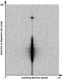
Figure 5: A dispersed image for an M type star, $V=10$ mag (with noise) as generated by the simulation software from Scholz (1998). Note the contribution of the zeroth order seen as a single intensity “blob” in the upper part of the image. The first, second and third spectral order are all overlapping (lower intensity “stretch”) due to the grating. The intensity stripes to the side of the dispersed image are due to diffraction at the telescope’s aperture.

Interstellar extinction was modelled by using a synthetic extinction curve for $R=3.1$ given as $\frac{A(\lambda)}{E(B-V)}$ versus $\lambda$. We used the extinction curve from Fitzpatrick (1999), simulating 7 different extinction values in steps of 0.15 and 0.2 in the range $0.0\leq\$$E(B-V)$$\ \leq 1.0$ mag. Note that the zeroth order was omitted in this and all other simulations, so that we only worked with dispersed images made up of the first to third spectral order. Since the data were area-normalized before passing them through the neural network, the magnitude information of the zeroth order is lost anyway. For the simulation of the UV-telescope (see below), the same extinction curve was applied. This procedure was done for five different visual magnitudes in the range from $8\leq\$V$\ \leq 12$ mag.

Noise was added to these two-dimensional intensity distributions by passing them through another software tool developed by Ralf Scholz. Here, a mean sky backround of $sky=0.04$e^-/(pix s) and a dark current of $dark=2$e^-/(pix s) were added with additional source and sky Poisson noise. The CCD’s read out noise was 2 e^-/eff.pix.

The size of the SC window to be cut from the on-board data stream around the dispi is crucial as it determines the data rate which is in turn related to the satellite’s overall performance: A smaller window permits a larger number of SC windows (objects) to be transmitted. This would, for example, permit a fainter magnitude limit. The optimum window size, i.e. the window around a dispersed image with the highest amount of important and lowest amount of redundant information, was investigated in earlier studies. Concerning the window size in the cross dispersion direction it was found that the innermost 7 pixel are sufficient (Hilker et al. 2001) in terms of highest S/N. However, due to the satellite’s intrinsic attitude uncertainty it is required that the smallest acceptable window size in the scanning direction be 12 pixel (see Bastian & Schilbach 2001). For our studies we therefore summed up the TDI-rows over the innermost 13 rows (6 pixels in each direction about the central row). Future work will use a profile fit to obtain the stellar intensity.

The optimum size in the dispersion direction was evaluated by S/N studies and the (spectral) information content. This amount of information was measured by the ability of Neural Networks to determine the stellar parameters $T_{\rm eff}$, $\log g$ and [M/H] for different ranges of dispis. It was found (Willemsen et al. 2001) that these parameters can be adequately retrieved from approximately 45 effective pixels around the maximum intensity in the dispis (which is at about effective pixel 60). However, since these earlier studies included only dispis with $T_{\rm eff}$$\geq$ 4000 K and since the overall intensity distribution moves to smaller effective pixel values for lower temperatures, we chose the range from 30 to 80 effective pixels in this work. This should also be appropriate for very red objects like L and M dwarfs with $T_{\rm eff}$$\simeq$ 1200–4000 K.

For further processing, the simulated sky was subtracted from the dispersed image by evaluating the background level from a single column in scanning direction next to the dispersed image.

The UV imaging telescope will make use of the same type of CCD’s as the main instrument. The UV magnitudes in the two different passbands next to the Balmer jump were calculated from the same synthetic spectra as described above, simply by integrating the flux in the ranges from 310 to 360 nm and 380 to 410 nm. Of course, the true filters will not have exactly square transmission curves, but this approximation is sufficient for a first analysis of the influence of the UV channel. The two UV flux values were fed into the network in three different ways. First, we calculated the $asinh$ of the flux ratio, i.e. $asinh(UV_{\rm short}/UV_{\rm long}$) (note that the $asinh$ - function is not undefined for negative values, in contrast to the log-function. Negative values might occur due to noise for very low temperature stars with almost no flux in the UV). This ratio is designed to be sensitive to the Balmer jump thus yielding additional information about gravity and temperature. Second, we summed up the intensity in a dispi in the range 70 to 80 effective pixel ($\sum_{i=70}^{80}I_{i}$) and calculated the ratios ($UV_{\rm short}/\sum_{i=70}^{80}I_{i}$) and ($UV_{\rm long}/\sum_{i=70}^{80}I_{i}$). Since the first order’s contribution in the selected effective pixel range corresponds to a wavelength range from about 550 to 600 nm (see Fig. 1), these ratios should be a good measure of extinction due to the long “lever” ranging from the UV to the visual/red part of the spectrum.

4.2 Noise in single DISPIs versus end of mission stacked DISPIs

The results reported in this paper (Sect. 6) have been obtained using single dispis. However, by the end of the mission, DIVA will have imaged each star about 120 times. Thus the final signal-to-noise ratio for any given magnitude will be much better than from a single measurement. Therefore, the parametrization performance will also be improved or, equivalently, will be achieved at a fainter magnitude. We calculate the final S/N from a sum of 100 two-dimensional intensity distributions. From the ratio of this final S/N to the single dispi S/N, we can find the equivalent magnitude difference which gives the magnitude to which our parametrization results for a single dispi can be applied to, without having to do a set of separate simulations on summed dispis. The resulting $\Delta V$ is given in Fig. 6 (see further Sect. 6). We see, for example, that a dispi made up of one-hundred frames each with $V=14$ mag has the same S/N as a single dispi of a star with magnitude $V=10.8$ mag. Unless stated otherwise, all results below will refer to end-of-mission data quality.

Figure 6: One-hundred added frames each of the ‘single’ visual magnitude given on the x-axis yield the same S/N as a star which is $\Delta V$ magnitudes brighter. For example, adding 100 frames of $V=14$ mag stars (two-dimensional intensity distributions) and calculating a dispi from these yields a dispi which has the same S/N as a single dispi of a star with $V=10.8$ mag. Clearly, for fainter stars, the noise is dominated by the read-out noise, while for brighter stars only the Poisson noise of the signal is relevant, thus yielding a full magnitude shift of 5 mag. This curve was calculated by making use of the specific DIVA’s CCDs noise characteristics.

5 Preparing the ANN input data

The ensemble of dispis was divided into several smaller samples with different temperature ranges. We chose seven different ranges with a broad distinction between low - (the L-samples), mid - (M-samples) and high temperatures (H-samples). The abbreviations as stated in Table 2 are used throughout this work. The numbers in the last column show the total number of dispis  in the training set in this temperature interval for the case without and with extinction included (approximately the same number of dispis in each temperature range was used in the application set.)

Table 2: Abbreviations, temperature ranges and number of dispis in the training sets, with and without extinction (the number in the application sets similar).

sample	temperature range	without/with ext.
L1	2000 K $\leq$ $T_{\rm eff}$$<$ 4000 K	330/2300
L2	4000 K $\leq$ $T_{\rm eff}$$<$ 6000 K	570/3980
L3	6000 K $\leq$ $T_{\rm eff}$$<$ 8000 K	500/3500
M1	8000 K $\leq$ $T_{\rm eff}$$<$ 10000 K	400/2800
M2	10000 K $\leq$ $T_{\rm eff}$$<$ 12000 K	180/1200
H1	12000 K $\leq$ $T_{\rm eff}$$<$ 20000 K	390/2700
H2	20000 K $\leq$ $T_{\rm eff}$$<$ 50000 K	450/3100

We found that the separation into such small temperature regions yielded improved parametrization results. This is understandable as the classification results for the stellar parameters, especially $\log g$ and [M/H], depend upon the presence of spectral features in a dispi which are also closely related to the temperature of a star. This effect was also found in Weaver & Torres-Dodgen (1997), using spectra in the near-infrared and classifying them in terms of MK stellar types and luminosity classes. For our ANN work we chose simple temperature ranges, also aiming at database subsamples of similar size. Though some of the intervals roughly correspond to the temperatures found in certain MK classes which are characterized by certain line-ratios, i.e. common physical characteristics, the chosen distinction was motivated to allow for a reasonable training time for the networks. Another reason was to see what can be learned from dispis in different temperature regimes in principle. The mid-temperature samples (M-samples) were defined for the range in which the Balmer jump and the H-lines (e.g. H_β) change their meaning as indicators for temperature and surface gravity (see e.g. Napiwotzki et al. 1993). Under real conditions one would have to employ a broad classifier to first separate dispis into smaller (possibly overlapping) temperature ranges. This could be also based on neural networks, but also on other methods, such as minimum distance methods. Each temperature sample was finally divided into two disjoint parts, the training- and the application data. This means that our classification results (see Sect. 6) are from dispis in the gaps of our training grid.

The generalization performance of a network or its ability to classify previously unseen data is influenced by three factors: The size of the training set (and how representative it is), the architecture of the network and the physical complexity of the specific problem, which also includes the presence of noise. Though there are distribution-free, worst-case formulae for estimating the minimum size of the training set (based on the so called VC dimension, see also Haykin 1999), these are often of little value in practical problems. As a rule of thumb, it is sometimes stated (Duda et al. 2000) that there should be (W $\cdot$ 10) different training samples in the training set, W denoting the total number of free parameters (i.e. weights) in the network. In our network without extinction there were 452 weights. Thus, in some cases, there were fewer training samples than free parameters. However, we found good generalization performance (see Sect. 6 and results therein). This may be due both to (1) the “similarity” of the dispis in a specific $T_{\rm eff}$ range, giving rise to a rather smooth (well-behaved) input-output function to be approximated, and (2) redundancy in the input space. Both give rise to a smaller number of effective free parameters in the network.

We also tested whether there are significant differences between determining each parameter separately in different networks and determining all parameters simultaneously. In the first case each network would have only one ouput node while in the latter case the network had multiple outputs. If the parameters ($T_{\rm eff}$, $\log g$ etc.) were independent of each other, one could train a network for each parameter separately. However, we know that the stellar parameters influence a stellar energy distribution simultaneously at least for certain parameter ranges, (e.g. hot stars show metal lines less clearly than cool stars). Also, for specific spectral features, changes in the chemical composition [M/H] can sometimes mimic gravity effects (see for example Gray 1992). Varying extinction can cause changes in the slope of a stellar energy distribution which are similar to those resulting from a different temperature.

Recently, Snider et al. (2001) determined stellar parameters for low-metallicity stars from stellar spectra (wavelength range from 3800 to 4500 Å). They reported better classification results when training networks on each parameter separately. We tested several network topologies with the number of output nodes ranging from 1 to 3 (in case of extinction from 1 to 4) in different combinations of the parameters. It was found that single output networks did not improve the results. We therefore classified all parameters simultaneously.

6 Results

In this section we report the results from our parameter determination. In order to appreciate the results one has to realize that the effects of $T_{\rm eff}$, $\log g$ and [M/H] on a spectrum differ significantly in magnitude. The strongest signal is that of temperature (the Planck function for black bodies). The much weaker signal is that of $\log g$, present in the width of spectral lines but only weakly in the continuum. Metallicity is a very weak signal visible in individual spectral lines or perhaps in broader opacity structures (such as G-band or molecular bands). However, in a dispi essentially all line structure is washed out. These general aspects can also be found in Gray (1992). For more see Sect. 7.

Figure 7: The average classification uncertainty for $T_{\rm eff}$, $\log g$ and [M/H] from top to bottom as a function of visual magnitude, V, plotted for the different temperature sets. No extinction was added for these simulations. The stated error is that of Eq. (1). The lower magnitude scale refers to end of mission data in which 100 dispis of objects with the magnitude given on the upper scale are stacked (see Fig. 6 for details). The lettering for the different temperature ranges refers to the temperature ranges given in Table 2. The left column shows the results for networks which were trained on dispis (with an effective pixel range from 30 to 80) including the UV channel fluxes for the particular star, while the right column shows results for those simulations without UV data. For [M/H] only the results for the temperature ranges L1 to L3 and [M/H]$\geq$ $-$0.3 dex are presented, as for higher temperatures and lower metallicities spectral information of this parameter is washed out at these resolutions.

The errors given are the average errors as in Eq. (1). $T_{\rm eff}$ was classified in terms of log $T_{\rm eff}$ but for better understanding, the resulting errors were transformed to give the fractional error in $T_{\rm eff}$. These fractional errors are stated throughout this paper.

The networks had the same overall topology for all tests, though the number of inputs naturally was three larger for the case with UV information. We did not tune the networks to the very best performance possible. Tests showed that results in individual $T_{\rm eff}$-ranges could be improved through adjustments of several free parameters in the networks (e.g. the number of hidden nodes, number of iterations etc.). In some cases, we had to adjust some of these parameters, for example in the cases that the networks did not converge properly. However, such individual tests are very time-consuming. For the purpose of this paper, we used one topology.

Fig. 7 shows the classification results for the stellar parameters $T_{\rm eff}$, $\log g$ and [M/H] in case of no extinction, while Fig. 8 presents the results for simulations with extinction included. For each plot, the left column shows the results when UV data were included, while the right column refers to the cases without additional UV data. The upper magnitude scale shows the visual magnitudes for a single detection, whereas the lower magnitude scale is relevant for a sum of 100 dispis, representative of end-of-mission quality data (see Fig. 6).

As a comparison, we tested the performances of random, i.e. untrained, networks. These are presented in Table 3. If trained networks give parameters with uncertainites larger than the values listed here, those parameter values are not meaningful. The corresponding error for $E(B-V)$ was about 0.25 mag for all temperature ranges and magnitudes.

Table 3: Performances of random (untrained) networks. The stated errors are the average errors as in Eq. (1) (the error for log $T_{\rm eff}$ is multiplied by 2.3 to give the fractional error). The errors only depend on the output parameters and are therefore the same for all magnitudes. If trained networks give parameters with uncertainites larger than the values listed here, those parameter values are not meaningful.

Param.	$A_{L1}^{*}$	$A_{L2}$	$A_{L3}$	$A_{M1}$	$A_{M2}$	$A_{H1}$	$A_{H2}$
$T_{\rm eff}$	0.15	0.1	0.07	0.06	0.05	0.15	0.17
$\log g$	1.9	1.4	1.3	1.0	0.8	0.8	0.6
[M/H]	1.2	1.8	1.8	-	-	-	-

^∗ Temperature ranges as in Table 2

A variation in [M/H] changes a dispi only very subtly for higher temperature stars due to the simple fact that metallicity features are very weak in the energy distribution of hotter stars.

7 Discussion and conclusions

As can be seen from Fig. 7 and 8 our results show interesting trends related with the temperature of the stars. In general, temperature is the dominating factor for the shape of and even the details in a spectral energy distribution. Overall, $T_{\rm eff}$ can be retrieved to very acceptable accuracy, even without additional UV information: the classification is better than 10 % even for very faint stars ($V=14$ mag, no extinction included: through this section the V magnitude refers to end-of-mission quality data). Including UV fluxes improves the $T_{\rm eff}$ parameter results most noticeably for hot stars ($T_{\rm eff}$$>$ 9000 K) and here especially for the fainter ones. For example, in case of no extinction, the error for dispis  with $V=14$ mag in the $T_{\rm eff}$ range 12000–20000 K (H1 sample) drops from 5 % to about 3 % when the UV data are included. When extinction is included, the temperature error drops from 9 % to about 4 % for this temperature range at this magnitude. Though the information in the short wavelength range is already available in the dispi, the higher sensitivity of the UV telescope obviously contributes essential information.

Figure 8: The same as in Fig. 7 but with extinction included. The left column shows the results for networks which were trained with UV data while the right column shows the classification results for tests without UV data.

Concerning $\log g$ we see from the figures that the classification performance can be improved when additional UV information is included. For example, in case of no extinction and for temperatures in the range 8000 K $\leq$ $T_{\rm eff}$ $<$ 10000 K (M₁) and visual magniude $V=14$, the error in $\log g$ reduces from about 0.4 to 0.15 dex with additional UV information. At this magnitude but for temperatures in the range 6000 K $\leq$ $T_{\rm eff}$ $<$ 8000 K (L₃), the error reduces considerably from about 0.85 dex to 0.15 dex. These results emphasize the benefit of UV telescope data in the classification process. In general, the $\log g$ results are poorer for temperatures in the range 4000 K $\leq$ $T_{\rm eff}$ $<$ 6000 K (L2 sample) when compared to other ranges. This is understandable since in this temperature range hardly any atomic/molecular signatures sensitive to the density (and thus $\log g$) of the gases in a stellar atmosphere are present. In contrast, for the very low temperature ranges the numerous mostly molecular spectral features provide the information about the density of the atmospheric gases. For the higher temperatures the Balmer jump provides still gravity information.

Metallicity is the most difficult parameter to derive from dispis. This was to be expected: In data with such low spectral resolution all details of spectral line information, and thus of metal abundances, are lost. In Figs. 7 and 8 only the classification results for metallicities in the range $-$0.3 dex to 1.0 dex are shown. This is due to a lack of input data in the metallicity range from $-$2.5 dex to $-$0.3 dex (see above). Very low metallicities ([M/H] $\leq$ $-$2.5 dex) make only a very small imprint on a dispi such that the classification almost fails completely at these resolutions, except for very bright, cool stars ($T_{\rm eff}$ $\leq$ 4000 K). The results for metallicities in the analysed metallicity range are reasonably good even for low magnitudes (better than about 0.3 dex for $V\leq 14$ mag, no extinction). When extinction is included, the metallicity performance declines considerably, except for the very cool objects ($T_{\rm eff}$ $<$ 4000 K, L1 sample) the metallicity of which can be determined to better than 0.3 dex for all simulated magnitudes. For dispis in the temperature range 6000 K $\leq$ $T_{\rm eff}$ $<$ 7000 K ($L_{3}$) we see that the error can be reduced from about 0.45 dex to 0.3 dex (no extinction) and from about 0.8 dex to 0.6 dex (with extinction) when the UV information is included.

Extinction is not easy to be retrieved solely from the shape of a dispi, since its overall effect mimics, to some extent, that of temperature. However, as can be seen from the figures, the determination of extinction improves when the UV information is included. This was to be expected since the UV data gives the strength of the Balmer jump, giving $T_{\rm eff}$ information unblurred by extinction.

One may ask whether the accuracy of the parameters derived would be better when working with the single orders of the DIVA dispersed image. We have tested this for a limited number of parameter combinations. We generally found that for brighter objects ($V\leq\ 13$ mag) the accuracy is improved when using the single orders and then only by a small amount (in the range 30 to 80 effective pixels). This might be surprising at first but it is understandable since for fainter objects, using the signal in a single order, deteriorates the S/N, so we find a poorer result from the parameter extraction routine. Apart from these results, to obtain the separate order’s signals would require a deconconvolution of the dispi which in itself leads to increased uncertainty in the intensities. Moreover, a deconvolution requires knowledge of the nature of the objects so there is no guarantee that this process will yield unique results. Since DIVA will not have separate order images we have not pursued this aspect further.

Several neural network approaches to stellar parametrization have been reported in astronomy. A comparison with those would have to address at least two aspects, such as nature of the type of network and characteristics of the data used. The networks may indeed be very different in structure such as learning and regularization technique and especially topology (compare e.g. Weaver & Torres-Dodgen 1995, Snider et al. 2001 and this work). But because in all these cases the data were of very different nature (e.g. different resolutions and number of input flux bins), a general comparison of the results is not really possible. A few remarks can be made nevertheless.

Projects to obtain MK classifications normally use data in the wavelength range from 3800 to 5200 Å with high spectral resolution of about 2 to 3 Å (see e.g. Bailer-Jones et al. 1998). Weaver & Torres-Dodgen (1995) and Weaver & Torres-Dodgen (1997) classified stars in terms of MK classes in the visual to near-infrared wavelength range 5800-8900 Å with a resolution of 15 Å. However, even the resolution of these spectra is still much better (by a factor of approx. three) than the “best” one of dispis which is about 40 Å in the low efficiency third order. We would expect such resolutions to give better precision for spectral type or $T_{\rm eff}$ as well as for line sensitive parameters ($\log g$ and [M/H]) than with dispis on account of the higher resolution. Snider et al. (2001) recently classified spectra having 1 to 2 Å resolution. They determined $T_{\rm eff}$, $\log g$ and [M/H] of low metallicity stars to an accuracy of about 150 K in $T_{\rm eff}$  in the range 4250 K $<$ $T_{\rm eff}$$<$ 6500 K, 0.30 dex in $\log g$ over the range $1.0\leq\$$\log g$$\ \leq 5.0$ dex and 0.20 dex in [M/H] for $-4\leq\$[M/H]$\ \leq 0.3$ dex. From our results, we find for this temperature range ($L_{2}$ and $L_{3}$ sample) a classification precision in $T_{\rm eff}$ of better than 5% for $V\leq 14$ mag (no extinction) without UV information and about 2% when UV data are included. Only for brighter stars ($V\leq 13$ mag) do we find that $\log g$ can be determined from dispis to better than 0.3 dex for temperatures in the range 4000 K $\leq$ $T_{\rm eff}$ $<$ 6000 K but only when UV data are included. Concerning metallicity, our results are comparable (better than 0.2 dex for visual magnitudes $V\leq\ 12$ mag, no extinction, UV data included). Clearly, this is because we have only used metallicities in the range from $-$0.3 dex to +1 dex (see above).

A comparison with the neural network approach using synthetic data for a test of possible GAIA photometric systems (Bailer-Jones 2000) may be of relevance. Bailer-Jones also used input data with various moderate resolutions, some of them similar to those of the spectral orders in dispis. The effects of the quantum efficiency (QE) of the detectors was not included, so that in his tests the information provided in the vicinity of (and shortward of) the Balmer jump could be utilized in full. After shifting our results to the fainter magnitudes reachable with GAIAs larger telescope, while considering the other differences between Bailer-Jones’ and our investigation as well as the differences between the DIVA and GAIA optics and data format, one must conclude that these ANN analyses work to similar satisfaction.

Little work has been done so far concerning the automated determination of interstellar extinction. Weaver & Torres-Dodgen (1995) tested the effect of extinction and found that $E(B-V)$ could be determined from spectra of A type stars with an accuracy of 0.05 mag in the range of $E(B-V)$ of 0 - 1.5 mag. Gulati et al. (1997) used IUE low-dispersion spectra (wavelength range 1153 - 3201 Å, spectral resolution 6 Å) from O and B stars. Applying reddening to their spectra in the $E(B-V)$ range of 0.05 - 0.95 mag in steps of 0.05 mag, they were able to retrieve extinction with high accuracy to about 0.08 mag, clearly because of the presence of the 2200 Å bump in the input data. From Fig. 8 we see that extinction can be determined from dispis to better than 0.08 mag for visual magnitudes $V\leq\ 14$ mag for all temperatures in case that UV data are included.

Concerning the DIVA satellite, Elsner et al. (1999) found interesting results with Minimum Distance Methods. However, the optical concept of DIVA has changed considerably since then. Thus, also here a comparison of the quality may lead to a skewed judgement and we therefore refrain from going into detail.

A final remark deals with the effect of selecting our training sample randomly from the database. A random selection may accidentally lead to larger regions of parameter space without training data. Since our object (“application”) sample is the complement of the training set, objects falling in those gaps clearly are classified worse than objects near trained points. Malyuto (2002) demonstrated such effects when using Minimum Distance Methods. The average errors in our results are influenced by such effects, but this was not investigated.

In considering the accuracies obtained with our ANN approach we have to note that real stellar spectra show a much more complex behaviour than synthetic ones. For example, even the more realistic approach of non-LTE models (Hauschildt et al. 1999) cannot properly describe the true behaviour of elements in a stellar atmosphere (see e.g. Gray 1992, Ch. 13). Moreover, good colour calibrations in accord with observed data are still difficult to obtain, as described e.g. in Westera et al. (2002). It is difficult to estimate how to properly weigh such intrinsic inconsistencies with respect to the final performance of the DIVA satellite. The effect of such cosmic scatter probably is that the final performance of DIVA might be less accurate than our results from these ideal synthetic spectra, or, that the accuracy curves of Fig. 7 and Fig. 8 are to be shifted somewhat to brighter magnitudes.

We argued that additional UV data can improve the parameter results considerably in the classification process. The spectral library of our present simulations does not include, however, changes in, e.g., alpha-process elements which can show up in changes also in the range of DIVA’s UV channels (e.g. the CN violet system in the range from 385 to 422 nm).

The conclusions of the discussion are
1) The ANN method is well suited to obtain astrophysical parameters from DIVA dispis.
2) The accuracy obtained is related with the strength of the signal of each parameter as present in a dispi: $T_{\rm eff}$ is best, followed by $\log g$, and then $E(B-V)$ and [M/H].
3) The accuracy is clearly related with temperature: toward higher temperature the signal of both $\log g$ and [M/H] decreases considerably.
4) Our results were obtained with synthetic spectra. Real stars will not all behave like text book objects and the classification coming from real data will necessarily be less good, albeit always to an unknown amount per star.
5) The classification quality is absolutely adequate to be able to select objects of desired characteristics from the final DIVA database to do statistical analyses and/or for efficient post mission type-related investigations.