The Quintuple Quasar: Mass Models and Interpretation

Abstract

The strange morphology of the six-component gravitational lens PMN J0134$-$0931 has resisted explanation. We present the first successful quantitative models for the system, based on the idea that there are two lens galaxies and two components of the background source. One source is quintuply imaged and corresponds to the five brightest observed radio components. The other source is triply imaged and corresponds to the sixth component, along with two others too faint to have been detected. The models reproduce the observed image positions and fluxes, and make falsifiable predictions about other properties of the system. Some of these predictions have been confirmed by high-resolution radio and optical observations, as described in the companion paper by Winn et al. (2003). Although we cannot determine the lens model uniquely with current data, we predict that the lens galaxies are spiral galaxies with roughly equal velocity dispersions $\sigma\sim 120\,\mbox{km~{}s${}^{-1}$}$ and a projected separation of only 0$\farcs$4 (2 $h^{-1}$ kpc at $z_{l}=0.76$). This system is the first known lens with five images of a single quasar, and the second with more than four images.

1 Introduction

The radio source PMN J0134$-$0931 presents a formidable challenge to the gravitational lensing theorist. Instead of having two or four images like nearly every other lensed quasar, the system has at least six components at radio wavelengths (Winn et al. 2002a; hereafter W02). The five brightest components (named A–E in order of radio flux density) have identical continuum radio spectra, but C and E were missing from a high-resolution 1.7 GHz map (W02) and also from optical and near-infrared images (Gregg et al. 2002; Hall et al. 2002; hereafter G02 and H02). Adding to the mystery, the object is one of the reddest quasars known ($B-K\geq 11$), but the location of the dust presumed to cause the reddening is unknown (G02; H02).

Confusion has reigned over such basic issues as the number of lensed images in the system. Four completely different lensing scenarios have been proposed. First, W02 pointed out that four of the components (A, B, D, and F) might be explained as a 2-image lens of a 2-component source, with C and E assumed to be foreground objects, but one would need to invoke coincidence to explain why C and E have the same spectral slope as A, B, and D. Second, W02 suggested that all six components could be images of a single source if there is more than one lens galaxy, but they did not present any quantitative models because the parameter space of multiple-galaxy models is large and not easily explored. Third, G02 imagined A, B, D, and E to constitute a standard 4-image lens, but admitted that such a scenario does not explain component C. Finally, H02 suggested that A–E are five images of a single source and F represents a different source. Although they did not present a quantitative model, H02 pointed out two features that would be expected of such a model: there must be at least two lens galaxies; and there would presumably be at least one additional image of the source corresponding to component F, which should be detectable with more sensitive radio observations.

Here we present a comprehensive lensing analysis of J0134$-$0931, concluding that the quintuple-imaging scenario is correct, and backing it up in quantitative detail. To do so, we originally used modeling considerations. We exhaustively searched the parameter space of two-galaxy lens models, finding numerous successful 5-image lens models but no good 6-image models. While this work was in progress, Winn et al. (2003; hereafter W03) discovered that the spectral index of component F is significantly different from that of the other components. This removed any motivation to consider 6-image models further. Furthermore, the multi-frequency maps of W03 showed that the lower surface brightness of C and E, which was the main objection to the H02 scenario, is due to scatter-broadening rather than being intrinsic. We therefore present only our results for the quintuple-imaging scenario.

Our approach was to search for mass models that could reproduce the most obvious and most easily quantified properties of the system—the number of radio components, their relative positions, and to some extent their relative fluxes (§2)—using two lens galaxies at the same redshift with unknown positions, masses, and shapes (§3). Our success (§4.1) obviated the need to consider more complicated (and a priori unlikely) models involving additional deflectors or deflectors at more than one redshift.

More interestingly, the two-galaxy models make strong predictions about aspects of the system that are observable but were not used as constraints. In particular, they specify the positions of the two galaxies (§4.2); the time delays between the images (§4.3); the resolved shapes of the images (§4.4); the existence of radio arcs (§4.5); and the existence of two “counter-images” of component F (§4.6). New radio and optical observations have been able to test and confirm some of these predictions, as described in the companion paper by W03. Overall, this analysis provides a lensing context that will be valuable for further interpretation of this complex and fascinating system (§5).

Throughout this paper we neglect any faint “core” images that would appear near the center of the lens galaxies; see Keeton (2003) for a general discussion of core images, and Rusin et al. (2001) for a discussion of the various combinations of bright and faint images possible when there are multiple galaxies. Where necessary we adopt a cosmology with $\Omega_{M}=0.3$ and $\Omega_{\Lambda}=0.7$, but changing the cosmology would have little effect on our results.

2 Constraints on lens models

The observed properties of J0134$-$0931 are summarized by W03. For modeling purposes, we adopted the relative image positions and flux ratios for components A–E from multi-frequency VLA and MERLIN maps by W02. The astrometric uncertainties from these data are 1–2 milli-arc seconds (mas). The VLBA maps have higher astrometric precision, but because small-scale structure in the lens potential can perturb the image positions by $\sim$1 mas (Mao & Schneider 1998; Metcalf & Madau 2001), sub-mas precision is not desirable in an analysis focusing on the kiloparsec-scale properties of the lens model. Because component F has only been detected in VLBA maps, we used the VLBA position of that component relative to D, and adopted a 2 mas uncertainty in each coordinate.

The optical flux ratios are best avoided as model constraints because of the contaminating influence of reddening by dust (G02; H02; W03). Instead we used the radio flux density ratios measured by W02. Although the statistical uncertainties in these ratios are 2–4%, we adopted a larger uncertainty of 10% in order to account for possible systematic effects. One particularly important systematic effect is small-scale structure in the lens potential; many studies have shown that mass clumps of size $10^{4}$–$10^{8}\,M_{\odot}$ can perturb radio flux density ratios by $\sim$10% or more (e.g., Mao & Schneider 1998; Metcalf & Madau 2001; Chiba 2002; Dalal & Kochanek 2002).

3 Methods

Single-galaxy models can produce lenses with more than four bright images, but only in configurations with an even number of images lying in a narrow annulus around the lens galaxy (Keeton et al. 2000a; Evans & Witt 2001), which is not the case for J0134$-$0931. The only way to produce more than four bright images in a different configuration is with more than one galaxy (Rusin et al. 2001). Our goal was to see whether two galaxies were sufficient to explain the configuration of J0134$-$0931, and if so, how well the galaxy properties could be constrained by the data.

We modeled the galaxies as singular isothermal ellipsoids (e.g., Kassiola & Kovner 1993; Kormann, Schneider & Bartelmann 1994; Keeton & Kochanek 1998). This is a widely-used model because it is consistent with the observed properties of other individual lenses, lens statistics, and the dynamics and X-ray properties of elliptical galaxies (e.g., Fabbiano 1989; Kochanek 1993; Maoz & Rix 1993; Kochanek 1996; Rix et al. 1997; Treu & Koopmans 2002). This assumption does not cause too much loss of generality; using a different radial mass profile would mainly rescale the predicted time delays (e.g., Kochanek 2002). In the absence of other information, we assumed that both galaxies lie at the absorption line redshift $z_{l}=0.76$ measured by H02. We also included a possible tidal shear due to additional objects near the galaxies or along the line of sight, because such shears seem to be common (e.g., Keeton, Kochanek & Seljak 1997; Holder & Schechter 2002).

The models had 15 free parameters: the positions, ellipticities, orientations, and masses of the two galaxies, the amplitude and orientation of the tidal shear, and the position and flux of S₁, the background source corresponding to A–E. The data provide 15 constraints: a position and flux for each of five images. We did not include component F (or its source component, S₂) as a constraint because it has no securely detected counter-images, but instead used it as an a posteriori test of the models (see §4.6). Thus, the models formally have zero degrees of freedom.

We used the lens modeling algorithm and software written by Keeton (2001b). For a given lens model, the software solves the lens equation to find the predicted image positions ${\bf x}_{i,{\rm mod}}$ and fluxes $f_{i,{\rm mod}}$, and compares them to the observed image positions ${\bf x}_{i,{\rm obs}}$ and fluxes $f_{i,{\rm obs}}$ using the goodness of fit statistic

$$\chi^{2}=\sum_{i=1}^{N_{\rm images}}\left[\frac{|{\bf x}_{i,{\rm mod}}-{\bf x}_{i,{\rm obs}}|^{2}}{\sigma_{i,x}^{2}}+\frac{(f_{i,{\rm mod}}-f_{i,{\rm obs}})^{2}}{\sigma_{i,f}^{2}}\right],$$ (1)

where the index $i$ runs over all the images, and $\sigma_{i,x}$ and $\sigma_{i,f}$ are the uncertainties in the positions and fluxes, respectively. Models that do not produce the correct number of images are penalized by setting $\chi^{2}$ to an extremely large value. The software varies the parameters of the model, using a downhill simplex optimization routine (e.g., Press et al. 1992) to minimize $\chi^{2}$ and find the best fit to the data.

For this particular problem, we used two special techniques to control the parameter search. First, to ensure a fair sampling of the large and complex parameter space, we ran the optimization many times starting from random points. We drew initial galaxy positions from a box enclosing the radio components, initial ellipticities from the range $0\leq e\leq 0.6$, and random initial orientations. Second, to speed up the optimization, we noted that it is possible to set up a system of linear equations for the optimal values for four of the parameters (see the Appendix). For any set of the 11 non-linear parameters one can simply solve the system of equations to find the best values for the four linear parameters. As a result, the parameter space that needs to be searched by the optimization routine has only 11 dimensions rather than 15. This technique has been used (in slightly different forms) by Kochanek (1991a, 1991b), Bernstein & Fischer (1999), and Keeton et al. (2000b). One possible problem is that the solutions of the linear equations actually optimize a quantity $\chi^{2}_{{\rm src}}$ that is usually a good approximation to the $\chi^{2}$ defined in eq. (1) but may have slightly different minima. Out of concern about this effect, we considered two approaches. In “assisted” models we used the linear parameter technique throughout the modeling process, whereas in “direct” models we used it when selecting the random starting points but not when optimizing the parameters. As discussed below, the two sets of models had similar properties, suggesting that the linear parameter technique did not significantly bias our results.

4 Results

4.1 Quality of the fits

We repeated our randomization and optimization modeling procedure many times to obtain a suite of lens models that sample the local minima in the $\chi^{2}$ surface. Figure 1 shows histograms of $\chi^{2}$ values for 50 assisted and 51 direct models with $\chi^{2}<30$. In this sample, there are four assisted models that give a perfect fit ($\chi^{2}=0$), and another four models (three assisted, one direct) with $\chi^{2}<1$. The existence of models that fit the data exactly is not mathematically surprising, because the models have zero degrees of freedom. It is nevertheless interesting to find physically plausible two-galaxy models that can account for the configuration of this unusual lens. Our first significant result is the mere existence of quantitatively successful models of J0134$-$0931.

Figure 1: Histogram of $\chi^{2}$ values for the models. The different histogram indicate different types of models. There are 50 assisted models and 50 direct models with $\chi^{2}<25$.

There are a few models with $1<\chi^{2}<8$, and a large collection of models (41 assisted, 48 direct) centered at $\chi^{2}\sim 16$. Interestingly, in the latter models most of the value of $\chi^{2}$ comes from the flux ratios (see Table 1). In fact, the dominant contribution is from the flux of component A, which is commonly predicted to be $\sim$40% fainter than observed. This is an important point, because recent theoretical work has indicated that in many lenses one of the image fluxes is perturbed by mass substructure in the lens (e.g., Mao & Schneider 1998; Metcalf & Madau 2001; Chiba 2002; Dalal & Kochanek 2002). According to such analyses, even smooth models that correctly describe the overall lens potential can fail to reproduce one of the flux ratios. The smooth models will often tend to underestimate the flux of the brightest image, which is exactly the situation for the $\chi^{2}\sim 16$ models.

Let us stress, though, that we do not claim that substructure is required to explain the radio flux ratios in this system. That claim is disproved by the existence of smooth models that fit the radio data exactly. Rather, we simply argue that models with $\chi^{2}\sim 16$ dominated by a $\sim$40% discrepancy in the flux of A should not be ruled out. We therefore consider all models with $\chi^{2}<25$ to be viable models. (This limit represents a natural break in the $\chi^{2}$ histograms; see Figure 1.) We study a sample of acceptable models containing 50 assisted models and 50 direct models.

Note that there is little difference between the $\chi^{2}$ histograms for assisted and direct models. The assisted models appear to be somewhat more efficient at finding models with $\chi^{2}<10$, presumably because the linear parameter technique helps the downhill simplex method find models that lie at the bottom of narrow valleys in the $\chi^{2}$ surface (see §3). But there is no significant and systematic difference in the values of $\chi^{2}$ or the best-fit parameter values between the two model types, which is reassuring evidence that the linear parameter technique did not bias our results.

4.2 Galaxy properties

Table 1 gives typical values of the model parameters for ten representative models, chosen to capture the range of properties seen in the full sample of 100 models. To give a visual impression of the range of positions, relative masses, ellipticities, and orientations for the lens galaxies, in Figure 2a we have overplotted the $\kappa=\Sigma/\Sigma_{\rm crit}=1$ contours for the two galaxies in all 100 models.

The first interesting result is that the models all basically agree on the positions of the two galaxies. The northern galaxy (henceforth labeled Gal-N) lies $\sim$0$\farcs$2 south of component C, while the southern galaxy (Gal-S) lies $\sim$0$\farcs$15 south of component E. The fact that the galaxy positions vary little from model to model indicates that they are robust predictions of two-galaxy models.

More details become apparent when the models are grouped by their $\chi^{2}$ values, as in Figure 2b–d. The best models ($\chi^{2}<1$) fall into two different families: either the two galaxies are both oriented nearly east–west, or they are both oriented nearly north–south. In the range $1<\chi^{2}<15$, the range of allowed ellipticities and orientations increases, and for some models Gal-N is allowed to be highly flattened in the north-south direction.

The models with $15<\chi^{2}<25$ represent the majority (84%) of allowed models, and form a remarkably homogeneous family that is qualitatively different from the other models. In all but one of these models, the galaxies are comparatively round and are located almost directly south of of components C and E. (Recall that these are the models that are acceptable under the hypothesis that mass substructure affects the radio flux density of A.)

A different way to display the model results is with scatter plots of the parameter values. Figure 3a provides this view of the galaxy positions. As before, it is evident that the models basically agree on the galaxy positions. There is some freedom for the galaxies to move through a $\sim$0$\farcs$1 range along lines running northwest to southeast, but as they move they must maintain a fixed separation of $0\farcs 385\pm 0\farcs 008$ (2.0 $h^{-1}$ kpc at $z_{l}=0.76$).

Figure 3b shows the allowed values of the galaxy mass parameters $b_{\rm Gal-N}$ and $b_{\rm Gal-S}$ (defined in eq. A2 in the Appendix). In most models the two galaxies have comparable masses, although there is some freedom to make one or the other galaxy more massive provided that the total mass within the region bounded by the images remains fixed. The mass parameter $b$ can be translated into a velocity dispersion via the relation $\sigma\approx 117\,(b/0\farcs 2)^{1/2}\,\mbox{km~{}s${}^{-1}$}$, assuming a lens redshift $z_{l}=0.76$ and neglecting an ellipticity-dependent factor of order unity.

Finally, Figures 3c and 3d show that there is great diversity in the allowed ellipticities and orientations of the two galaxies. The models fill a broad region in these slices of parameter space. We therefore cannot determine these aspects of the lens models from the image configuration alone, although some discrimination may be possible from observations of the intrinsic, resolved shapes of the individual images (see §4.4).

When G02 deconvolved a ground-based $K^{\prime}$-band image, they found two faint components in addition to A, B, and D. They suggested that, if these components were real and not deconvolution artifacts, they might correspond to component E and a lens galaxy. Because the positions of these peaks agree well with the two predicted galaxy positions, we suggest instead that G02 detected both of the lens galaxies.

Furthermore, H02 identified possible flux from a lens galaxy or galaxies in Hubble Space Telescope (HST) images but were unable to draw any detailed conclusions. In a more careful analysis of the HST images that was conducted in tandem with this work, W03 found clear evidence for two flux peaks. The peaks agree roughly with the positions predicted by the models, although imperfect PSF subtraction makes it difficult to measure their positions accurately.

Thus, the $K^{\prime}$-band and optical HST images appear to confirm the first important prediction of the models, the presence of two galaxies near components C and E. It is interesting to note that the southern peak observed by W03 in the HST images appears to be elongated in the east–west direction. In principle, one might use this information to rule out the broad class of models that predict Gal-S to be round or elongated north–south. However, we hesitate to rule out models based on the HST images, not only because the residual peaks are faint and poorly characterized, but also because the mass distribution need not follow the light distribution. Differences between the mass and light distributions would not be surprising of the two galaxies are interacting, or if they are spiral galaxies (as we suspect) with prominent spiral arms.

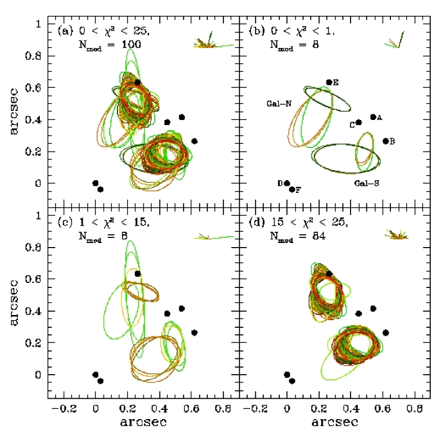
Figure 2: Isodensity contours ($\kappa=1$) of the two lens galaxies, drawn for various lens models. The vectors in the upper right corner indicate the amplitude and direction of the external shear. The points represent the observed radio components. (a) All 100 acceptable models. (b)–(d) Models in different $\chi^{2}$ ranges as indicated in the key, where $N_{{\rm mod}}$ is the number of models shown.

Figure 3: Scatter plots of parameter values for acceptable models. (a) Galaxy positions; Gal-S is shown as squares and Gal-N as triangles. The circles indicate the positions of components A–E. (b) The mass parameters $b_{\rm Gal-N}$ and $b_{\rm Gal-S}$. (c) Ellipticity and position angle for Gal-S. (d) Ellipticity and position angle for Gal-N. In all cases, large (small) points correspond to models that are consistent (inconsistent) with the observed 15 GHz shapes of the images at 95% confidence (see §4.4).

4.3 Components A–E

The lensing properties of this system can be understood by examining the critical curves, caustics, and time delay surface, which are shown in Figure 4. (To avoid clutter only the ten models listed in Table 1 are shown, but the other models are qualitatively similar.) Although there is some freedom for the critical curve to meander, especially to the southeast near component D, the data require the critical curve to thread between A, B, C, and E along a well-constrained path. Components A and D both lie outside the critical curve and at minima of the time delay surface, so they are predicted to have positive parity; while B, C, and E all lie inside the critical curve and at saddle points of the time delays surface, so they are expected to have negative parity. These results have implications for the resolved shapes of the images (see §4.4).

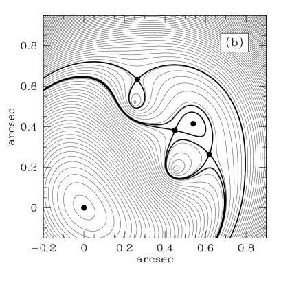
Figure 4: (a) Critical curves for the ten models in Table 1. The circles show the positions of components A–E, while the crosses indicate the positions of component F and its predicted counter-images. (b) Time delay surface for a typical model. The light contours are spaced by 0.25 $h^{-1}$ days, while the heavy contours are drawn to pass through the saddle points (images B, C, and E). (c) Caustics for the ten models in Table 1, in coordinates centered on S₁ (circle). The crosses indicate the position of the source component S₂. (d) Full caustic structure for a typical model. The numbers in the form $N_{\rm tot}/N_{\rm bri}$ show the total number of lensed images $N_{\rm tot}$ and the number of bright (non-core) images $N_{\rm bri}$ for sources in the different regions of the source plane.

The models all predict that S₁, the source corresponding to components A–E, lies only $\sim$0$\farcs$02 from a cusp in the caustic (Figure 4b). The models also generally agree on the position and orientation of that cusp, and on the presence of a second cusp nearby. There is less agreement about the shape of the caustic farther from the source, which corresponds to the poorly-constrained stretch of the critical curve. The fact that the source lies so close to a cusp means that the quasar host galaxy might be visible as a partial or complete Einstein ring in a high-resolution near-IR image of the system (see Kochanek, Keeton & McLeod 2001).

One feature of J0134$-$0931 cited by W02 as circumstantial evidence for gravitational lensing was the fact that four of the radio components (A, B, D, and F) lie on a circle, and that the A/B radio arc conforms closely to the same circle. However, as our models do not involve an intrinsically circular mass distribution, we suggest that the near-perfect circularity is just a mild coincidence. Any three points (say, A, B, and D) define a circle. Any extended emission should be seen most prominently between A and B because they are the brightest images. The extended emission, along with any additional images near D, are likely to lie in the direction of maximum stretching in the image plane, which is roughly perpendicular to the A–D separation.

The differential time delays between the images can be predicted from the models. In all cases the temporal ordering of the images, from shortest time delay to longest, is D–A–C–B–E. The delay values are shown in Figure 5, using the source redshift $z_{s}=2.2$ and assuming that the galaxies lie at redshift $z_{l}=0.76$. The delays are short because the angular size of the lens is small. The D–A delay is only $\sim$10 days ($\sim\!7\,h^{-1}$ days), and the A–E delay is only another $\sim$2 days. The small separations between components A, B, and C mean that the time delays between them are just a few hours.

Figure 5: Histograms of the predicted time delays between various image pairs.

Little or no variability has been measured in the total radio flux density over a 20-year baseline (W02), which is reason for pessimism about the prospect of measuring the time delays at radio wavelengths. One might hope for a greater degree of variability at optical or near-infrared wavelengths. The time delays would be challenging to measure at these wavelengths because of the small angular size of the system, but G02 demonstrated that it is possible to resolve some of the components in ground-based images with reasonable accuracy. Another possibility is to attempt to measure the short delays between A, B, and C in a single X-ray observation; the general feasibility of this approach has been demonstrated by Dai et al. (2001), but it would depend on the X-ray flux of the quasar. Although the complexity of J0134$-$0931 makes it unlikely ever to be useful for Hubble constant determination, measurements of the time delays would provide valuable new constraints on lens models.

4.4 Resolved image shapes

In high-resolution VLBA observations, W03 resolved the five radio components A–E. Although we did not use this information to derive our lens models, we can use it as an a posteriori test of the models. Specifically, we considered the images shapes inferred from elliptical Gaussian fits to the 15 GHz VLBA maps. We chose 15 GHz to minimize the possible effect of scatter-broadening, and we used only the position angles (rather than the major and minor axes) because the true 15 GHz shapes are not simply ellipses. For modeling purposes, we used an elliptical source, because it can easily be combined with the lensing magnification tensor to estimate the orientation of the lensed image (Keeton 2001a). It ought to be reasonable to compare predicted orientations of images inferred from an elliptical source to the measured orientations, even if the images are not strictly elliptical.

For each of the 100 lens models we varied the axis ratio and orientation of the source component S₁ to find the best fit. The best case has $\chi^{2}_{\rm shape}=0.58$ for three degrees of freedom. A total of 23 models are consistent with the data at better than 95% confidence ($\chi^{2}_{\rm shape}<7.8$ for three degrees of freedom). These models all have sources with an axis ratio between 1.5 and 2.0 and position angle between $145\arcdeg$ and $153\arcdeg$.

The fact that 77 of our otherwise successful models are formally excluded by the image shapes indicates that the shapes contain important higher-order information about the lensing potential. It reassures us that the remaining 23 models are reasonable descriptions of the potential. It also narrows the range of allowed lens galaxy properties. Figure 3 shows that the models that agree with the images shapes occupy smaller regions of parameter space than the full set of models. Specifically, the two galaxies must lie at the western end of the allowed range of positions (and hence due south of components C and E), and Gal-N must be moderately elongated north–south. Interestingly, the image shapes seem to exclude models in which Gal-S is elongated east–west, suggesting that its mass distribution may not follow its light distribution (see §4.2).

We caution, however, against over-interpreting the $\chi^{2}_{\rm shape}$ values because fitting the complex 15 GHz image shapes with elliptical Gaussians probably underestimates the uncertainties in the position angles (see W03). We consider the models that produce formal agreement to be favored, but do not consider the other models to be ruled out definitively.

4.5 Extended emission

W02 detected a curved arc of radio emission at 1.7 GHz between components A and B. Again, because we did not use this information to derive our lens models, we can use it as an independent check of the models. At 15 GHz, the angular sizes of A–E are no greater than a few milli-arcseconds and no arcs are seen (W03), both of which imply an angular size of $\sim$1 mas for S₁. At lower frequencies, though, one might expect the source to be larger and any extended emission (which typically has a steeper radio spectrum than the core) to be more prominent. As a first step, we took the model that gives the best fit to the 15 GHz image shapes and enlarged the angular size of S₁ to 15 mas. The result is shown in Figure 6a.

Figure 6: Images of an elliptical source centered on S₁ with axis ratio 1.8 and position angle $148\fdg 5$ (panel a) or $58\fdg 5$ (panel b). The contours correspond to isophotes at 0$\farcs$005, 0$\farcs$010, and 0$\farcs$015 along the major axis.

The model predicts extended emission between components A and B, and also between components A and C. These two predictions appear to be robust and common to models that reproduce the 15 GHz image shapes, although the detailed surface brightness profiles of the A/B and A/C extended emission depend on the angular extent, orientation, and shape of S₁. The bright A/B arc discovered by W02 is therefore compatible with the models. In addition, W03 found evidence for a connection between components A and C.

However, Figure 6a is not the best possible fit to the surface brightness distributions observed by W03. The model predicts the A/B emission to lie nearly along a straight line, but it is actually curved along a nearly circular arc. In addition, the model predicts the A/C emission to have nearly the same brightness as the A/B emission, but it is apparently fainter (although scatter broadening at 1.7 GHz may contribute to the difference).

Trying to optimize the model to fit the extended emission would require a detailed description of the surface brightness distribution plus a much more sophisticated modeling algorithm, and is beyond the scope of this paper. Instead, we simply note that a better fit to the data is obtained when S₁ is rotated by $90\arcdeg$. The results for that case are shown in Figure 6b. The A/C arc is now fainter and the A/B arc is curved, as observed. This model has the additional virtue that the major axis of S₁ points nearly in the direction of S₂, which is what one would expect for a core-jet source. In this scenario, S₂ is neatly explained as a hot-spot in the $\sim$15 mas jet emerging from S₁.

Taken at face value, the analyses of the 15 GHz image shapes and the 1.7 GHz extended emission suggest that the jet is bent by $\sim$90 degrees between its emergence from S₁ on scales of $\lesssim$1 mas and its continuation to S₂ on scales of $\sim$15 mas. This might seem unnatural, but in fact bends of this size have been observed within the inner few milli-arcseconds of active galactic nuclei (e.g., Kellerman et al. 1998), and are usually explained as a smaller three-dimensional bend angle viewed nearly along the jet axis.

4.6 Component F

Component F, with its steeper spectral index (W03), corresponds to a different source component in our models that we call S₂. According to the models there should be additional lensed images of S₂ that have not yet been detected. To learn about these counter-images of F, we used each of the 100 allowed models to map F into the source plane, locating S₂. We then solved the lens equation for S₂ to find the positions and fluxes of all images besides F. Figures 4 and 7 show the positions of S₂ and the counter-images. Figure 8 is a histogram of the separation between S₁ and S₂. Finally, Figure 9 shows the predicted fluxes of the counter-images relative to F.

Figure 7: Predicted positions of the counter-images of F near component C (left) and E (right). The circles show components C and E, while the crosses show the predicted counter-images ${\rm C}^{\prime}$ and ${\rm E}^{\prime}$ for the 100 acceptable lens models.

Figure 8: Histogram of the inferred separation between the two sources S₁ and S₂.

Figure 9: Histograms of flux ratios (relative to F) for the predicted counter-images of F. The open and light shaded histograms denote ${\rm E}^{\prime}$ and ${\rm C}^{\prime}$, respectively, for our full set of 100 models. The heavy shaded histograms are for the subset of models that are consistent with the 15 GHz image shapes.

All but one of the models predict that S₂ lies just outside the cusp caustic and hence produces three images. Thus, F should have two counter-images that lie close to components C and E. It is striking that even though F lies only 0$\farcs$05 from D, and even though S₂ is only $\sim\!0\farcs 015$–$0\farcs 020$ from S₁, and even though no information about F or its counter-images was used to derive the models, nearly all of the models predict that F belongs to a family of images with a different multiplicity than A–E. In the one exception, S₂ lies just inside the cusp caustic and F has four counter-images: one near C, one near E, and a pair straddling the critical curve between A and B. The existence of (at least) two counter-images of F is therefore a robust and testable prediction of the models.

We refer to putative counter-images near C and E as ${\rm C}^{\prime}$ and ${\rm E}^{\prime}$, respectively. We reserve the names G and H, which would follow from the flux-order convention by which A–F are named, for any actual detections of these components. This is partly because the predicted flux ordering is not certain, although generally F is predicted to be brighter than ${\rm C}^{\prime}$, which in turn is brighter than ${\rm E}^{\prime}$. In the majority of cases, ${\rm C}^{\prime}$ is 80–90% as bright as F (especially for models that agree with the measured 15 GHz image shapes; see Figure 9), while ${\rm E}^{\prime}$ is only $\sim$25% as bright as F.

Given that ${\rm C}^{\prime}$, in particular, is predicted to be only modestly fainter than F, one might expect that it could easily be detected or ruled out. Unfortunately, circumstances make detection of the counter-images difficult and obscure the interpretation of non-detections. Because of the steep radio spectrum of S₂, one would prefer to search for ${\rm C}^{\prime}$ and ${\rm E}^{\prime}$ at low radio frequencies where their flux densities are large. However, at low radio frequencies, C and E are heavily scatter-broadened, suggesting that ${\rm C}^{\prime}$ and ${\rm E}^{\prime}$ might also be broadened out of detectability. Given the high electron column density implied by the scatter-broadening, it is also possible that the flux of these components is being reduced by free-free absorption. At high radio frequencies, where these plasma effects are smaller, the counter-images are predicted to be intrinsically faint.

These challenges are illustrated by the analysis of new high-resolution VLBA maps by W03. In the 1.7 GHz map, component C is missing, because of scatter-broadening and possibly free-free absorption. Intriguingly, however, there is a puff of resolved emission located just south of the expected position of C, which is exactly where ${\rm C}^{\prime}$ is predicted to appear. The total flux of the extended emission is $\approx$90% of the flux of F at that frequency, which is also consistent with the prediction for ${\rm C}^{\prime}$. It is therefore possible that W03 detected ${\rm C}^{\prime}$. But if the figure of 90% is correct, then W03 should also have detected ${\rm C}^{\prime}$ at 8.4 GHz (where it should have been much more compact due to the $\nu^{-2}$-dependence of scatter-broadening) and they did not.

If ${\rm C}^{\prime}$ and ${\rm E}^{\prime}$ were point sources at 8.4 GHz, and if scatter-broadening were neglected, the 5$\sigma$ upper limits of the map would imply $S/S_{\rm F}<0.57$ for both counter-images. The limit on ${\rm E}^{\prime}$ is consistent with all the models, but the limit on ${\rm C}^{\prime}$ formally excludes 96% of our otherwise acceptable models, including all the models that agree with the 15 GHz image shapes. However, if ${\rm C}^{\prime}$ and ${\rm E}^{\prime}$ were scatter-broadened even at 8.4 GHz, the upper limits would be weakened. For example, under the assumption that ${\rm C}^{\prime}$ and ${\rm E}^{\prime}$ have the same ratio of peak to total flux density as C and E, respectively, the 8.4 GHz upper limits would become $S_{{\rm C}^{\prime}}/S_{F}<2.1$ and $S_{{\rm E}^{\prime}}/S_{F}<1.1$, which are consistent with all of our models.

Thus, it appears that the new observations by W03 were not conclusive in this regard. This is unfortunate, because the detection of a counter-image would be a clear validation of the models. Probably the best strategy for future attempts to detect the counter-images is to conduct more sensitive VLBI observations at around 8 GHz, where the plasma effects are expected to be small, and the intrinsic flux density of S₂ is still fairly large. If the sensitivity could be improved by a factor of $\sim$3, then ${\rm C}^{\prime}$ should be revealed; if by a factor of $\sim$10, then ${\rm E}^{\prime}$ should also be revealed. However, because the plasma effects cannot be quantified without assumptions about the density, temperature, and path length through the ionized material, a non-detection would be difficult to interpret unless one worked at 15 GHz or higher, where the observed angular sizes of C and E appear to be mainly intrinsic.

5 Discussion

The observed properties of the unique gravitational lens J0134$-$0931 can be completely explained as follows. The background radio source has two components, S₁ and S₂, separated by $\sim$15–20 mas (90–120 $h^{-1}$ pc at $z_{s}=2.2$). Source S₁ is the radio core with a gigahertz-peaked radio spectrum and a quasar optical counterpart (W02; G02). Source S₂ has a steeper radio spectrum (W03) and is a hot-spot in a jet emerging from S₁. The jet is bent, turning by $\sim\!90\arcdeg$ from its emergence from S₁ ($\lesssim$1 mas) to its continuation towards S₂ ($\sim$15 mas).

There are two lens galaxies in the foreground producing five images of S₁ (observed as radio components A–E) and three images of S₂ (of which only F has been securely detected, although W03 found evidence for one additional image). The $\sim$10 mas jet between S₁ and S₂ is magnified into the extended emission observed at low frequencies between A and B, and between A and C. The inner $\lesssim$1 mas of the jet is displayed in the resolved image shapes at 15 GHz.

The lens galaxies have nearly equal mass ($\sigma\sim 120\,\mbox{km~{}s${}^{-1}$}$) and are seen in projection just south of components C and E. Due to ionized material in the northern galaxy, components C and E (and, to a lesser degree, component A) are being scatter-broadened at radio wavelengths (W03). Due to differential reddening by dust in both galaxies, the optical counterparts of the images have different colors (H02; W03). The inference of large amounts of dust and ionized material leads us to suspect that the galaxies are spiral galaxies.

We have shown that this scenario can account quantitatively for the observed positions and relative fluxes of the radio components. In addition, W03 have presented evidence for the direct detection of the lens galaxies in HST images, in agreement with an earlier detection of two flux peaks by G02 in a $K^{\prime}$-band deconvolution. A subset of our models are also compatible with the intrinsic image orientations measured by W03, and with the upper limits on the flux densities of the counter-images of component F (although there are potential ambiguities in the interpretation of both constraints).

Two puzzles remain. First, many of our models, and especially those that are consistent with the 15 GHz image shapes, predict that the radio flux density of component A should be $\sim$40% lower than observed. It is possible that a small-scale density fluctuation in the lens model near image A is enhancing its flux density via the substructure lensing effect (e.g., Mao & Schneider 1998; Metcalf & Madau 2001). The density fluctuation might represent a mass clump such as a dark matter subhalo or globular cluster, or perhaps a tidal tail if the two lens galaxies are interacting. Although we cannot test this hypothesis with the present analysis, it may be possible to do so with a detailed study of the intrinsic shape of image A (see Metcalf 2002).

Second, our models suggest that the mass in the southern galaxy (Gal-S) cannot be highly elongated in the east–west direction and still be consistent with the observed 15 GHz image shapes. The puzzle is that there are two indications that Gal-S is indeed elongated east–west: the HST detection of Gal-S appears to be elongated east–west (W03); and component D is highly reddened (H02; W03), suggesting it is being covered by an easterly extension of Gal-S. Taking all this evidence seriously requires that the light and dust do not follow the mass. Although this might be unexpected, it does not demand an exotic explanation. There may simply be a spiral arm covering D. Or perhaps Gal-S has a dark matter halo that is fairly round but a light distribution that is flattened (such as an edge-on disk). Alternatively, perhaps the two galaxies are interacting and the relationship between light and mass is looser than for isolated galaxies, with the presence of tidal tails for example. In such a case, our assumption of ellipsoidal mass distributions would be incorrect, and future studies of this lens would need to consider a wider range of mass distributions.

J0134$-$0931 is the second galaxy-mass gravitational lens system with an image multiplicity larger than four. The first such system was the six-image lens B1359+154 produced by a compact group of three galaxies (Rusin et al. 2001). In both cases, the high multiplicity is due to the presence of more than one lens galaxy. It is interesting to note that both systems have a very compact arrangement of galaxies, smaller than the typical massive ellipticals that dominate lensing. In J0134$-$0931 the two galaxies have velocity dispersions $\sigma\sim 120\,\mbox{km~{}s${}^{-1}$}$ and a projected separation of just $0\farcs 4$ (2 $h^{-1}$ kpc at $z_{l}=0.76$), while in B1359+154 the three galaxies have $\sigma\sim 140$–$160\,\mbox{km~{}s${}^{-1}$}$ and a maximum projected separation of $0\farcs 7$ (4 $h^{-1}$ kpc at $z_{l}\sim 1$; Rusin et al. 2001). Although these are just two out of nearly 100 lenses currently known, they represent a much larger fraction of the radio surveys that discovered them; B1359+154 is one of 22 lenses in the Cosmic Lens All-Sky Survey (see Myers et al. 1999; Browne et al. 2001), while J0134$-$0931 comes from a survey that has found four lenses and one other candidate (Winn et al. 2000, 2001, 2002a, 2002b). The incidence of high-multiplicity lenses is still subject to Poisson uncertainties, but it appears to be several percent or even higher. Lensing, especially radio lens surveys, may therefore turn out to be an interesting way to discover compact groupings of galaxies at redshifts out to $z\sim 1$.

Appendix A Handling Linear Parameters

The surface mass density of an isothermal ellipsoid lens galaxy can be written as follows, in units of the critical density for lensing, and in a coordinate system aligned with the major axis of the ellipse:

$$\kappa(x,y)=\frac{\Sigma(x,y)}{\Sigma_{\rm crit}}=\frac{\sqrt{1+q^{2}}}{2\sqrt{2}\,q}\ \frac{b}{\sqrt{x^{2}+y^{2}/q^{2}}}\ ,$$ (A1)

where $q=1-e\leq 1$ is the axis ratio of the ellipse, and $b$ is a mass parameter. For a spherical galaxy, $b$ equals the Einstein radius and is related to the velocity dispersion $\sigma$ of the galaxy as

$$b=4\pi\left(\frac{\sigma}{c}\right)^{2}\frac{D_{ls}}{D_{os}}\ ,$$ (A2)

where $D_{ls}$ and $D_{os}$ are, respectively, angular diameter distances from the lens and observer to the source. For a non-spherical galaxy, this relation is modified by an ellipticity-dependent factor of order unity (see Keeton et al. 1997). Note that the surface mass density, and hence the lensing potential and deflection, is linear in $b$. This leads to an expression for the deflection of the form (see Kassiola & Kovner 1993; Kormann et al. 1994; Keeton & Kochanek 1998)

$${\bf\alpha}({\bf x};b,{\bf x}_{g},e,\theta_{e})=b\,\hat{\bf\alpha}({\bf x};{\bf x}_{g},e,\theta_{e})\,,$$ (A3)

where $\hat{\bf\alpha}$ is some function of position ${\bf x}$ in the image plane that depends on the parameters ${\bf x}_{g}$, $e$, and $\theta_{e}$ (the centroid, ellipticity, and orientation of the ellipsoid).

If we map an observed image ${\bf x}_{i}$ to the source plane using the two-galaxy-plus-shear model, we find the corresponding source position

$${\bf u}_{i}={\bf x}_{i}-b_{1}\,\hat{\bf\alpha}_{1}({\bf x}_{i};{\bf x}_{g1},e_{1},\theta_{e1})-b_{2}\,\hat{\bf\alpha}_{2}({\bf x}_{i};{\bf x}_{g2},e_{2},\theta_{e2})-\Gamma\cdot{\bf x}_{i}\,,$$ (A4)

where the two components $\gamma_{c}$ and $\gamma_{s}$ of the shear enter through the tensor

$$\Gamma=\left[\begin{array}[]{rr}\gamma_{c}&\gamma_{s}\\ \gamma_{s}&-\gamma_{c}\\ \end{array}\right].$$ (A5)

We might imagine that instead of evaluating $\chi^{2}$ by comparing the observed and predicted images in the image plane (eq. 1), we could simply work in the source plane and use the scatter in the model source positions, defining

$$\chi^{2}_{{\rm src}}=\sum_{i=1}^{N_{\rm images}}\frac{|{\bf u}_{i}-{\bf u}_{{\rm mod}}|^{2}}{\sigma_{i,x}^{2}}\ ,$$ (A6)

where ${\bf u}_{{\rm mod}}$ is the model source position. This “source-plane $\chi^{2}$” is often a good approximation to the image-plane $\chi^{2}$ and can be valuable for modeling (see Kochanek 1991a). We do not use it as the basis of all modeling mainly because it does not have the ability to check whether the model predicts the correct number of images, which is essential in the case of J0134$-$0931.

The important point is that the parameters $b_{1}$, $b_{2}$, $\gamma_{c}$, $\gamma_{s}$, and ${\bf u}_{{\rm mod}}$ are all linear parameters in $\chi^{2}_{{\rm src}}$. It is therefore possible to write down a system of linear equations for the parameter values that minimize $\chi^{2}_{{\rm src}}$. These equations have the form

$${\rm M}\cdot{\bf p}={\bf v}\,,$$ (A7)

where ${\bf p}=(b_{1},b_{2},\gamma_{c},\gamma_{s},u_{{\rm mod}},v_{{\rm mod}})$ is the parameter vector, and the matrix and right-hand side vector are:

$${\rm M}=\sum_{i=1}^{N_{\rm images}}\frac{1}{\sigma_{i,x}^{2}}\left[\begin{array}[]{cccccc}\hat{\bf\alpha}_{1x}^{2}+\hat{\bf\alpha}_{1y}^{2}&&&&&\\ \hat{\bf\alpha}_{1x}\hat{\bf\alpha}_{2x}+\hat{\bf\alpha}_{1y}\hat{\bf\alpha}_{2y}&\hat{\bf\alpha}_{2x}^{2}+\hat{\bf\alpha}_{2y}^{2}&&&&\\ x_{i}\,\hat{\bf\alpha}_{1x}-y_{i}\,\hat{\bf\alpha}_{1y}&x_{i}\,\hat{\bf\alpha}_{2x}-y_{i}\,\hat{\bf\alpha}_{2y}&x_{i}^{2}+y_{i}^{2}&&&\\ y_{i}\,\hat{\bf\alpha}_{1x}+x_{i}\,\hat{\bf\alpha}_{1y}&y_{i}\,\hat{\bf\alpha}_{2x}+x_{i}\,\hat{\bf\alpha}_{2y}&0&x_{i}^{2}+y_{i}^{2}&&\\ \hat{\bf\alpha}_{1x}&\hat{\bf\alpha}_{2x}&x_{i}&y_{i}&1&\\ \hat{\bf\alpha}_{1y}&\hat{\bf\alpha}_{2y}&-y_{i}&x_{i}&0&1\\ \end{array}\right]$$ (A8)

$${\bf v}=\sum_{i}\frac{1}{\sigma_{i,x}^{2}}\left[\begin{array}[]{c}x_{i}\,\hat{\bf\alpha}_{1x}+y_{i}\,\hat{\bf\alpha}_{1y}\\ x_{i}\,\hat{\bf\alpha}_{2x}+y_{i}\,\hat{\bf\alpha}_{2y}\\ x_{i}^{2}-y_{i}^{2}\\ 2x_{i}y_{i}\\ x_{i}\\ y_{i}\\ \end{array}\right]$$ (A9)

where $(\hat{\bf\alpha}_{1x},\hat{\bf\alpha}_{1y})$ and $(\hat{\bf\alpha}_{2x},\hat{\bf\alpha}_{2y})$ are the $x$ and $y$ components of the (scaled) deflections for galaxy 1 and 2, respectively, evaluated at the appropriate image position ${\bf x}_{i}$; and the sum is over the images. All the elements of ${\rm M}$ can be derived from the ones presented here, because ${\rm M}$ is symmetric.

Using standard methods to solve this system of equations (e.g., Press et al. 1992), we can find the optimal values of the parameters ${\bf p}$ given any values of the other model parameters. This technique can be used to aid the optimization as discussed in §3. In practice, we use only the values for $b_{1}$, $b_{2}$, $\gamma_{c}$, and $\gamma_{s}$ recovered from this analysis, even though solving the system of equations yields an estimate of the source position as well.

Table 1: Sample Model Parameters

Type	$b$ (″)	$x_{g}$ (″)	$y_{g}$ (″)	$e$	$\theta_{e}$ (∘)	$\gamma$	$\theta_{\gamma}$ (∘)	$\chi^{2}_{\rm pos}$	$\chi^{2}_{\rm flux}$	$\chi^{2}_{\rm shape}$
assisted	0.15	0.50	0.18	0.64	$11.5$	0.34	$96.3$	0.09	13.06	2.58
	0.14	0.25	0.47	0.86	$4.6$
assisted	0.16	0.49	0.19	0.54	$15.4$	0.27	$96.0$	0.04	14.07	0.58
	0.16	0.25	0.49	0.80	$5.2$
assisted	0.20	0.45	0.19	0.09	$108.2$	0.05	$66.7$	0.03	16.38	5.59
	0.19	0.25	0.52	0.33	$16.9$
assisted	0.18	0.47	0.21	0.40	$49.3$	0.11	$113.5$	0.03	15.35	7.56
	0.17	0.26	0.53	0.66	$21.9$
assisted	0.18	0.47	0.20	0.29	$36.3$	0.11	$98.1$	0.01	15.18	2.06
	0.18	0.25	0.52	0.59	$13.1$
direct	0.17	0.48	0.19	0.40	$4.6$	0.18	$85.6$	0.02	14.17	2.85
	0.18	0.23	0.48	0.62	$178.5$
direct	0.19	0.46	0.20	0.10	$38.6$	0.06	$83.1$	0.08	16.16	3.06
	0.19	0.24	0.51	0.41	$12.4$
direct	0.18	0.47	0.20	0.21	$9.6$	0.11	$82.8$	0.02	15.46	1.22
	0.19	0.24	0.50	0.51	$2.9$
direct	0.19	0.46	0.20	0.10	$50.0$	0.06	$84.5$	0.03	15.64	4.08
	0.19	0.25	0.51	0.44	$13.3$
direct	0.19	0.47	0.20	0.25	$42.7$	0.09	$102.1$	0.02	15.52	3.75
	0.18	0.25	0.52	0.56	$18.8$

Note. — Parameters for five assisted and five direct models, randomly chosen among models consistent with the 15 GHz image shapes (see §4.4). The mass parameter $b$ is defined in eq. (A2) in the Appendix. The positions $(x_{g},y_{g})$ of the galaxies are measured relative to component D. The ellipticity $e$ and shear $\gamma$ are dimensionless. The orientation angles $\theta_{e}$ and $\theta_{\gamma}$ are given as position angles measured East of North. The goodness of fit statistics $\chi^{2}_{\rm pos}$, $\chi^{2}_{\rm flux}$, and $\chi^{2}_{\rm shape}$ refer to the image positions, the flux ratios, and the image shapes, respectively.

References

- (1)
- (2) Bernstein, G., & Fischer, P. 1999, AJ, 118, 14
- (3)
- (4) Browne, I. W. A. 2001, in ASP Conf. Ser. 237, Gravitational Lensing: Recent Progress and Future Goals, ed. T. Brainerd & C. S. Kochanek (San Francisco: ASP), 15
- (5)
- (6) Chiba, M. 2002, ApJ, 565, 17
- (7)
- (8) Dai, X., Chartas, G., Garmire, G. P., & Bautz, M. W. 2001, in AAS Meeting 199
- (9)
- (10) Dalal, N., & Kochanek, C. S. 2002, ApJ, 572, 25
- (11)
- (12) Evans, N. W., & Witt, H. 2001, MNRAS, 327, 1260
- (13)
- (14) Fabbiano, G. 1989, ARA&A, 27, 87
- (15)
- (16) Gregg, M. D., Lacy, M., White, R. L., Glikman, E., Helfand, D., Becker, R. H., & Brotherton, M. S. 2002, ApJ, 564, 133 (G02)
- (17)
- (18) Hall, P. B., Richards, G. T., York, D. G., Keeton, C. R., Bowen, D. V., Schneider, D. P., Schlegel, D. J., & Brinkmann, J. 2002, ApJ, 575, L51 (H02)
- (19)
- (20) Holder, G., & Schechter, P. 2002, preprint (astro-ph/0209532)
- (21)
- (22) Kassiola, A., & Kovner, I. 1993, ApJ, 417, 459
- (23)
- (24) Keeton, C. R., Kochanek, C. S., & Seljak, U. 1997, ApJ, 482, 604
- (25)
- (26) Keeton, C. R., & Kochanek, C. S. 1998, ApJ, 495, 157
- (27)
- (28) Keeton, C. R., Mao, S., & Witt, H. J. 2000a, ApJ, 537, 697
- (29)
- (30) Keeton, C. R., Falco, E. E., Impey, C. D., Kochanek, C. S., Lehár, J., McLeod, B. A., Rix, H.-W., Muñoz, J. A., & Peng, C. Y. 2000b, ApJ, 542, 74
- (31)
- (32) Keeton, C. R. 2001a, ApJ, 562, 160
- (33)
- (34) Keeton, C. R. 2001b, preprint (astro-ph/0102340)
- (35)
- (36) Keeton, C. R. 2003, ApJ, 582, 17
- (37)
- (38) Kochanek, C. S. 1991a, ApJ, 373, 354
- (39)
- (40) Kochanek, C. S. 1991b, ApJ, 382, 58
- (41)
- (42) Kochanek, C. S. 1993, ApJ, 419, 12
- (43)
- (44) Kochanek, C. S. 1996, ApJ, 466, 638
- (45)
- (46) Kochanek, C. S., Keeton, C. R., & McLeod, B. A. 2001, ApJ, 547, 50
- (47)
- (48) Kochanek, C. S., 2002, ApJ, 578, 25
- (49)
- (50) Kormann, R., Schneider, P., & Bartelmann, M. 1994, A&A, 284, 285
- (51)
- (52) Mao, S. & Schneider, P. 1998, MNRAS, 295, 587
- (53)
- (54) Maoz, D., & Rix, H.-W. 1993, ApJ, 416, 425
- (55)
- (56) Metcalf, R. B., & Madau, P. 2001, ApJ, 563, 9
- (57)
- (58) Metcalf, R. B. 2002, ApJ, 580, 696
- (59)
- (60) Myers, S. T., et al. 1999, AJ, 117, 2565
- (61)
- (62) Press, W. H., Teukolsky, S. A., Vetterling, W. T., & Flannery, B. P. 1992, Numerical Recipes in C: The Art of Scientific Computing (2d Ed.; New York: Cambridge Univ. Press)
- (63)
- (64) Rix, H.-W., de Zeeuw, P. T., Carollo, C. M., Cretton, N., & van der Marel, R. P. 1997, ApJ, 488, 702
- (65)
- (66) Rusin, D., et al. 2001, ApJ, 557, 594
- (67)
- (68) Schneider, P., Ehlers, J., & Falco, E. E. 1992, Gravitational Lenses (Berlin: Springer)
- (69)
- (70) Treu, T., & Koopmans, L. V. E. 2002, ApJ, 575, 87
- (71)
- (72) Winn, J. N., et al. 2000, AJ, 120, 2868
- (73)
- (74) Winn, J. N., Hewitt, J. N., Patnaik, A. R., Schechter, P. L., Schommer, R. A., López, S., Maza, J., & Wachter, S. 2001, AJ, 121, 1223
- (75)
- (76) Winn, J. N., Lovell, J. E. J., Chen, H.-W., Fletcher, A. B., Hewitt, J. N., Patnaik, A. R., & Schechter, P. L. 2002a, ApJ, 564, 143 (W02)
- (77)
- (78) Winn, J. N., Morgan, N. D., Hewitt, J. N., Kochanek, C. S., Lovell, J. E. J., Patnaik, A. R., Pindor, B., Schechter, P. L., & Schommer, R. A. 2002b, AJ, 123, 10
- (79)
- (80) Winn, J. N., Kochanek, C. S., Keeton, C. R., & Lovell, J. E. J. L. 2003, preprint (W03)
- (81)