Photoelectric heating and [CII] cooling in translucent clouds:
results for cloud models based on simulations of compressible MHD turbulence

Abstract

Far–ultraviolet (FUV) photons expel electrons from interstellar dust grains and the excess kinetic energy of the electrons is converted into gas thermal energy through collisions. This photoelectric heating is believed to be the main heating mechanism in cool HI clouds. The heating rate cannot be directly measured, but it can be estimated through observations of the [CII] line emission, since this is believed to be the main coolant in regions where the photoelectric effect dominates the heating. Furthermore, the comparison of the [CII] emission with the far–infrared (FIR) emission allows to constrain the efficiency of the photoelectric heating, using model calculations that take into account the strength of the radiation field. Recent [CII] observations carried out with the ISO satellite have made this study possible.

In this work we study the correlation between FUV absorption and FIR emission using three–dimensional models of the density distribution in HI clouds. The density distributions are obtained as the result of numerical simulations of compressible magneto–hydrodynamic turbulence, with rms sonic Mach numbers of the flow ranging from subsonic to highly supersonic, $0.6\leq M_{\rm S}\leq 10$. The FIR intensities are solved with detailed radiative transfer calculations. The [CII] line radiation is estimated assuming local thermodynamic equilibrium where the [CII] line cooling equals the FUV absorption multiplied by the unknown efficiency of the photoelectric heating, $\epsilon$.

The average ratio between the predicted [CII] and FIR emissions is found to be remarkably constant between different models, implying that the derived values of $\epsilon$ should not depend on the rms Mach number of the turbulence. The comparison of the models with the empirical data from translucent, high latitude clouds yields an estimate of the photoelectric heating efficiency of $\epsilon\sim$2.9$\times 10^{-2}$, based on the dust model of Li & Draine. This value confirms previous theoretical predictions.

The observed correlation between [CII] and FIR emission contains a large scatter, even within individual clouds. Our models show that most of the scatter can be understood as resulting from the highly fragmented density field in turbulent HI clouds. The scatter can be reproduced with density distributions from supersonic turbulence, while subsonic turbulence fails to generate the observed scatter.

1 Introduction

In diffuse interstellar clouds ($A_{\rm V}\lesssim 1$) the gas is heated mainly by photoelectrons expelled from dust grains by far–ultraviolet (FUV) photons (de Jong, 1977; Draine, 1978; Bakes & Tielens, 1994; Weingartner & Draine, 2001b) in the energy range 6 eV$<h\nu<$13.6 eV. The high energy limit corresponds to the cut–off in the FUV radiation field caused by the hydrogen absorption ($h\nu$=13.6 eV), while the low energy limit corresponds to the energy needed to free electrons from the grains ($h\nu\sim$6 eV). In the cold neutral medium ($T_{\rm kin}\lesssim 200$ K) photoelectric heating accounts for most of the heating, the X-ray and cosmic ray heating rates being more than an order of magnitude smaller (Wolfire et al., 1995). In a relatively dense neutral medium ($n_{\rm H}\gtrsim$100 cm^-3), where a significant fraction of carbon is in the neutral form, carbon ionization becomes an important heating source, but it is still not comparable to the photoelectric effect.

The efficiency of the photoelectric heating, $\epsilon$, is defined as the ratio between the kinetic energy of photoelectrons available to heat the gas and the FUV energy absorbed by the grains. Bakes & Tielens (1994) estimated the photoelectric yield to be close to 10%, meaning that of all the photons absorbed by grains only one in ten ionizes them. Furthermore, since the average absorbed photon has an energy of $\sim$8 eV and the work function for a neutral grain is $\sim$5.5 eV, only one third of the absorbed energy goes into the kinetic energy of the electron. The overall efficiency is therefore expected to be close to 3%, at least in the cold neutral medium. The rate decreases as the grains become positively charged. In the intense FUV radiation field of photodissociation regions, for example, the efficiency can be more than a factor of ten lower than in the cold neutral medium.

Ingalls et al. (2002) have recently studied a sample of translucent, high latitude clouds (HLCs). The [C⁺] 158 $\mu$m line ${}^{2}P_{3/2}\rightarrow^{2}P_{1/2}$ was observed with ISO and this was correlated with FIR intensities. In the cold neutral medium the [CII] line dominates the cooling (Wolfire et al., 1995), neutral carbon being the next most important coolant. Ingalls et al. (2002) estimated that for these clouds the CI cooling rate is at most 30% of the [CII] cooling rate and the CO rate is more than one order of magnitude smaller. Therefore, for the observed HLCs the [C⁺] 158$\mu$m line should account for at least 60% of the cooling and in most lines of sight the percentage should be considerably higher.

To be a tracer of photoelectric heating the [CII] emission must originate from the same regions where the photoelectric effect is the main heating source and, conversely, all regions where the photoelectric heating is dominant must be cooled predominantly by the [CII] emission. As discussed by Ingalls et al. (2002), both conditions are approximately satisfied. The ionization potential of carbon, 11.3 eV, is above the work function of grains, and therefore C⁺ exists only in regions where photoelectric heating is possible. Conversely, in regions where C⁺ is not present and C and CO are significant coolants, the photoelectric heating rate must be much lower than in regions where C⁺ is present. As in Ingalls et al. (2002) we therefore assume that the above conditions are satisfied and the photoelectric heating is exactly balanced by the [CII] line cooling.

Since all the FUV radiation in the energy range 6 eV$<h\nu<$13.6 eV absorbed by grains contributes to the photoelectric heating, the efficiency $\epsilon$ of this heating mechanism can be computed as the ratio of the observed [CII] line emission and the absorbed FUV radiation. If dust properties are assumed to be known, the absorbed FUV radiation can be estimated through the observed FIR emission. The problem of estimating $\epsilon$ is therefore reduced to the problem of computing the correlation between the absorbed FUV radiation and the observable FIR emission. Such correlation depends on both the intensity of the radiation field and the column density and can be determined with model calculations. The degeneracy between the effect of the column density and of the intensity of the the external radiation field could in principle be broken using the information contained in the shape of the spectral energy distribution. This requires, however, quite precise modeling of the dust emission.

Ingalls et al. (2002) modeled their observations using a plane parallel geometry. The FIR emission was calculated with a dust model consisting only of grains at equilibrium temperature. A comparison with [CII] and FIR observations resulted in an estimate of $\epsilon=0.043$ for the efficiency of the photoelectric heating. The average radiation field, $\chi$, was estimated to be above the local interstellar radiation field (ISRF), $\chi\sim 1.6\chi_{0}$, where $\chi_{0}$ refers to the sum of the 2.7 K cosmic background and the spectrum given by Mezger et al. (1982) and Mathis et al. (1983).

In the present work we follow the same approach as in Ingalls et al. (2002), in the sense of deriving theoretical relations between the FUV absorption and the FIR emission and then using the empirical relation between [CII] and FIR intensities to estimate the average efficiency of the photoelectric heating. However, our models of the FUV absorption and FIR emission is significantly more detailed and realistic than in Ingalls et al. (2002). We compute the radiative transfer on cloud models based on three dimensional numerical simulations of compressible magneto–hydrodynamic turbulence. The density distribution of these turbulent flows provides a realistic model for the density inhomogeneity of interstellar clouds (Padoan et al., 1997a, b, 1998, 1999; Padoan & Nordlund, 1999). The penetration of FUV radiation into the cloud depends on the cloud structure. Inside an inhomogeneous cloud the intensity of short wavelength radiation is higher than inside a homogenous cloud. Furthermore, density variations generate a significant scatter in the relation between the local FUV absorption and FIR emission. Our model can therefore be used to estimate what fraction of the observed scatter can be attributed to the inhomogeneous nature of the density field. Other factors that could also contribute to the observed scatter, such as anisotropy in the radiation field or abundance variations, are not considered. Other improvements of our work, compared with Ingalls et al. (2002), are related to the employed dust model. We use the three component model of Li & Draine (2001). The FIR intensities are calculated using the method of Juvela et al. (2003) and the emission from transiently heated dust grains is included.

2 The cloud models

The density distributions of the models are the result of three dimensional simulations of super–Alfvénic, compressible, magneto–hydrodynamic (MHD) turbulence. Three models are used, from three simulations with different values of the rms sonic Mach number of the flow, $M_{\rm S}=0.6$, 2.5 and 10.0 in model $A$, $B$, and $C$, respectively.

The simulations are carried out on a staggered grid of 250³ computational cells, with periodic boundary conditions. Turbulence is set up as an initial large scale random and solenoidal velocity field (generated in Fourier space with power only in the range of wavenumbers $1\leq K\leq 2$) and maintained with an external large scale random and solenoidal force, correlated at the largest scale turn–over time. The initial density and magnetic field are uniform and the gas is assumed to be isothermal. Details about the numerical method are given in Padoan & Nordlund (1999).

Experiments are run for approximately 10 dynamical times in order to achieve a statistically relaxed state. The cloud models used in this work correspond to the final snapshot of each simulation. The value of $M_{\rm S}$ is varied in different experiments by varying the thermal energy. The initial rms Alfvénic Mach number remains unchanged, $M_{\rm A}=10.0$, from run to run. The volume–averaged magnetic field strength is constant in time because of the imposed flux conservation. The magnetic energy is instead amplified. The initial value of the ratio of average magnetic and dynamic pressures is $\langle P_{\rm m}\rangle_{\rm in}/\langle P_{\rm d}\rangle_{\rm in}=0.005$ for all runs, so all the runs are initially super–Alfvénic. The value of the same ratio at later times is larger, due to the magnetic energy amplification, but still significantly lower than unity (0.21, 0.14 and 0.12 for models $A$, $B$ and $C$ respectively). The turbulence is therefore super–Alfvénic at all times.

Supersonic and super–Alfvénic turbulence of an isothermal gas generates a highly inhomogeneous gas density distribution, with a density contrast of several orders of magnitude. It has been shown to provide a good description of the dynamics of molecular clouds and of their highly fragmented nature (Padoan et al., 1997a, b, 1998, 1999; Padoan & Nordlund, 1999). Translucent high latitude clouds (HLCs), such as the ones observed by Ingalls et al. (2002), have been studied thanks to their CO emission (Magnani et al., 1996). Despite their lower gas density and presumably larger fraction of gas in the atomic form, the clouds can still be approximately modeled with an isothermal equation of state. At densities above 1 cm^-3 the gas temperature is expected to remain mostly in the range 50–100 K (e.g. Wolfire et al., 1995). The observed clouds are characterized by supersonic turbulent motions like denser molecular clouds (see e.g. Miesch et al., 1999). It seems therefore appropriate to use supersonic turbulence as a model not only of dense molecular clouds, but also of more diffuse clouds, such as the ones studied in this work. A subsonic model (model $A$) is also used in this work for the purpose of studying the effect of varying $M_{\rm S}$ over a large range of values.

To compute the radiative transfer the data cubes of the density distributions are scaled to physical units by fixing the length of the computational grid, $L=6.0$ pc, and the average hydrogen density, $\langle n_{\rm H}\rangle=100$ cm^-3. However, the radiative transfer calculations apply to all values of $L$ and $\langle n_{\rm H}\rangle$ satisfying the condition that their product is constant, $L\,\langle n_{\rm H}\rangle=600$ pc cm^-3= $1.8\times 10^{21}$ cm^-2. The column density in the models varies between different lines of sight, because of the inhomogeneous density field. Variations are particularly large in model $C$, where the range of column density values is comparable to that found in the Ingalls et al. (2002) sample. This can be seen for example by comparing the FIR intensities in the models and in the observations (see Sect. 4). When results are compared with observations, the angular size of the models (or their distance) must be fixed as well, in order to take into account the spatial resolution of the observations. One cell, 6.0/250 pc, is assumed to correspond to 0.25$\arcmin$, setting the model clouds at the distance of 330 pc.

3 Calculation of FUV absorption and FIR emission

Radiative transfer calculations are needed to obtain estimates for the [CII] emission and the total FIR emission along different lines of sight through the model clouds. Calculations are carried out on the original grid of 250³ cells. The external radiation field is assumed to be the local interstellar radiation field near the Sun (Mathis et al., 1983). The dust model is taken from Li & Draine (2001). This includes silicate grains (sizes $a>3.5$ Å), graphite grains ($a\gtrsim 50$ Å) and PAHs (from $a=3.5$ Å  to $\sim 50$ Å) with ionization state corresponding to physical conditions in the cold neutral medium (see also Juvela et al., 2003).

Following Ingalls et al. (2002) we assume explicitly a balance between the cooling by [CII] line emission and the photoelectric heating. The latter is taken to be equal to the dust absorption in the energy range 6–13.6 eV multiplied by the efficiency of the photoelectric emission, $\epsilon$. The penetration of the external radiation field is simulated with Monte Carlo methods, and the absorption in the given energy range is stored in each cell. The emerging [CII] intensity is calculated by summing the corresponding emission on selected lines–of–sight, assuming the emission is optically thin. The efficiency of the photoelectric heating is unknown but since it is assumed to be constant troughout the cloud it can be taken into account later in the analysis.

The dust emission was calculated using the ‘library method’ discussed in Juvela et al. (2003). First a mapping between the strength of the local radiation field at a few reference frequencies and the resulting dust emission is established. The radiation field at the reference frequencies is then simulated and the emission is obtained using the existing mapping. The emission, including the contribution from transiently heated particles, can be estimated with an accuracy of a few per cent even in the case of large three–dimensional models (see Juvela et al., 2003). The infrared emission from the clouds is estimated using this method. Ingalls et al. (2002) calculated FIR emission based on 60$\mu$m and 100$\mu$m values using the formula

$$I_{\rm FIR}=12.6\,\frac{I(100\mu m)-2.58\,I(60\mu m)}{\rm MJy\,sr^{-1}}\times 10^{-6}\frac{\rm erg}{\rm cm^{2}\,s\,sr}.$$ (1)

The formula gives the FIR emission between 42.5 $\mu$m and 122.5 $\mu$m i.e. the wavelength range covered by the IRAS 60$\mu$m and 100$\mu$m filters (Helou et al., 1985). In our models the formula was found to be accurate to $\sim 2-3$ per cent. However, the quoted FIR intensities are here calculated by direct integration over the computed spectra.

Both the FUV absorption (equivalent to the [CII] emission divided by the efficiency, $I_{\rm CII}/\epsilon$) and the FIR intensity, $I_{\rm FIR}$, are calculated towards three directions perpendicular to the faces of the cubic cloud. For each direction, maps of 250$\times$250 positions are generated. Results are compared with observations presented by Ingalls et al. (2002). The ISO LWS observations of the [C⁺] 158$\mu$m line have a resolution of 71$\arcsec$. The FIR data are based on IRAS ISSA maps with a resolution of $4-5\,\arcmin$. We assume the cells of our models have an angular size of 0.25$\arcmin$, and the computed [CII] and FIR maps are convolved to the resolution of the observations.

4 Results

4.1 FIR and [CII] emission in model clouds

For each model the FUV absorption and the FIR intensity, $I_{\rm FIR}$ are calculated towards three directions perpendicular to the faces of the density field data cubes. Since the FUV absorption is assumed to be equivalent to the [CII] line intensity, $I_{\rm CII}$, divided by the efficiency, $\epsilon$, in the following we will refer to the quantity $I_{\rm CII}/\epsilon$ (with $\epsilon$ still unknown), instead of the computed FUV absorption.

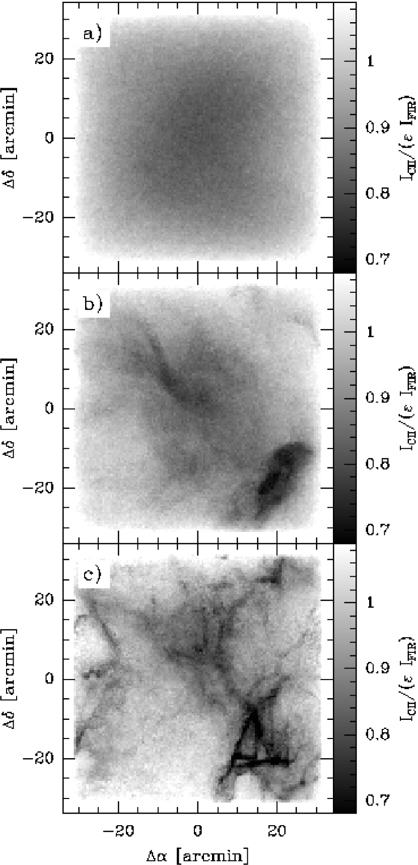
Figure 1: The ratio $I_{\rm CII}/(\epsilon I_{\rm FIR})$ in the three model clouds $A$, $B$ and $C$ (from top to bottom). The maps correspond to observations towards the $y$–direction. No convolution has been applied to either $I_{\rm CII}/\epsilon$ or $I_{\rm FIR}$ data.

Fig. 1 shows the distribution of the ratio $I_{\rm CII}/(\epsilon I_{\rm FIR})$ in the three models. The figure is obtained at the original resolution (250$\times$250 pixels), and neither $I_{\rm FIR}$ nor $I_{\rm CII}/\epsilon$ are spatially convolved. Model $A$ is based on a flow with subsonic turbulence, with only small density fluctuations. This is reflected in the top panel of Fig. 1 showing a smooth distribution of $I_{\rm CII}/(\epsilon I_{\rm FIR})$ in model $A$. The density contrast increases with increasing $M_{\rm S}$. Model $B$, with $M_{\rm S}=2.5$, shows a more ‘clumpy’ distribution of $I_{\rm CII}/(\epsilon I_{\rm FIR})$ (middle panel of Fig. 1). Model $C$, with $M_{\rm S}=10$, has clearly the most inhomogeneous and filamentary distribution (bottom panel of Fig. 1).

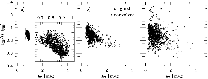
Figure 2: The ratio $I_{\rm CII}/(\epsilon I_{\rm FIR})$ as a function of the visual extinction along the line of sight. The three panels, a, b and c, correspond to the three models, $A$, $B$ and $C$ respectively. The figures show values calculated from the models towards the $y$–direction. The relations are shown for both the original data (dots) and the convolved data (crosses). For model $A$ the indicated area has been plotted also on a larger scale.

In the case of the nearly homogeneous cloud $A$, both $I_{\rm FIR}$ and $I_{\rm CII}/\epsilon$ are determined mainly by the distance to the cloud surface. Since $I_{\rm CII}/\epsilon$ is assumed to be equivalent to the FUV absorption, $I_{\rm CII}/\epsilon$ depends only on photons in the energy range 6–13.6 eV, while $I_{\rm FIR}$ depends on a much wider wavelength range responsible for heating the dust grains. The dust extinction increases towards shorter wavelengths, and this leads to a reduction in the ratio $I_{\rm CII}/(\epsilon I_{\rm FIR})$ inside the clouds. At the cloud surface the ratio $I_{\rm CII}/(\epsilon I_{\rm FIR})$ is above one, and it decreases to $\lesssim$0.8 inside the cloud, in all three models. The total range of values is wider in the more inhomogeneous clouds, with the lowest values reached in the highest density peaks. The average ratios are, however, very similar in all three models, $\langle I_{\rm CII}/(\epsilon I_{\rm FIR})\rangle\approx$0.9. The average value depends, of course, on the total column density and it would become lower in more opaque clouds. The models have similar column densities as the clouds in the sample of Ingalls et al. (2002), and if the clouds are subjected to similar radiation field as the models the exact correspondence can be checked by comparing the FIR intensities.

In Fig. 2 we plot the ratio $I_{\rm CII}/(\epsilon I_{\rm FIR})$ against the visual extinction of the corresponding line of sight. The average optical depth of the model clouds is below one, but the total range of $A_{\rm V}$ values depends on the degree of inhomogeneity. While in model $A$ the visual extinction stays below $\sim$1^m, the other models include a number of lines of sight with $A_{\rm V}$ in excess of 2^m (model $B$) and 3^m (model $C$). The figure shows the results for both unconvolved data and for the case where data have been convolved to the resolution of the observations (71$\arcsec$ for [CII] and $\sim$4$\arcmin$ for FIR data). The $A_{\rm V}$ data has not been convolved. This would correspond to a situation where the extinction is derived from photometry of an individual background star, probing only a single line of sight inside the larger beam employed in the other observations.

The negative correlation between extinction and the ratio $I_{\rm CII}/(\epsilon I_{\rm FIR})$ is clearly visible in model $A$ (Fig. 2a). In model $B$ the correlation can be seen in the unconvolved data, while in the convolved data the large difference between the resolution of the [CII] and FIR observations increases the scatter and the correlation becomes weak. At high extinction values the convolution increases systematically the $I_{\rm CII}/(\epsilon I_{\rm FIR})$ values. The [CII] intensity depends on FUV absorption, and because of the high optical depth the [CII] emission is likely to saturate near the column density maxima. Since the intensity distribution is already flat the convolution has little effect on the peak [CII] intensities. The FIR emission is less saturated and, more importantly, the FIR intensities are convolved with a beam that is several times larger. As the the FIR peaks are smoothed away the ratio $I_{\rm CII}/(\epsilon I_{\rm FIR})$ increases. The effect is even higher in model $C$ because of the stronger density contrast. However, in model $C$ the $A_{\rm V}$–dependence is quite weak even in the unconvolved data. This can be attributed to other effects related to the increased density contrast. For example, dense filaments and sheets are common, with the result that the $A_{\rm V}$ along one line of sight can be much higher than the average extinction by which the material is shielded towards other directions. In the figure this results in a larger scatter along the $A_{\rm V}$ axis.

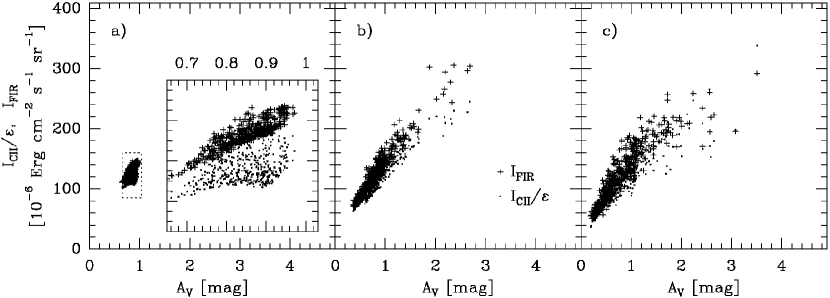
Figure 3: The convolved quantities $I_{\rm CII}/\epsilon$ and $I_{\rm FIR}$ as a function of visual extinction. The three panels, a, b and c, correspond to the three models, $A$, $B$ and $C$ respectively. For model $A$ the indicated area has been plotted also on a larger scale.

In a homogeneous model the extinction of the external radiation field proceeds in a predictable fashion, and the ratio between optical and FUV intensities only depends on the distance from the cloud surface. In an inhomogeneous cloud there is no longer a one–to–one relation between the shape of the spectral energy distribution and the intensity of the radiation. The FUV radiation penetrates deeper into the cloud than in the homogeneous model, and the variation in the ratio between optical and FUV intensities becomes smaller. If the cloud consisted of optically very thick clumps, the incoming radiation would have exactly the same spectral energy distribution at the centre of the cloud as on the surface – only the intensity would be smaller. MHD models are somewhere between the two extremes, that is between a homogeneous cloud and a cloud with optically thick clumps. In different parts of the cloud the spectrum of the radiation field may be different even for the same ‘effective extinction’ and this increases the scatter along the $I_{\rm CII}/(\epsilon I_{\rm FIR})$–axis.

In Fig. 3 the dependence on the visual extinction along the line of sight is shown separately for $I_{\rm CII}/\epsilon$ and $I_{\rm FIR}$. This shows explicitly the saturation of the [CII] emission, which at high column densities is caused by the total absorption of incoming FUV intensity. The [CII] line itself is assumed to be optically thin. The effect is particularly clear in model $B$. It is present also in model $C$, but it is partially masked by the scatter resulting from the more inhomogeneous cloud structure and the effects of the convolution.

Inhomogeneity is expected to lead to a decrease in total energy absorption (see Juvela et al., 2003) and, therefore, to lower the emitted intensities. The FIR emission in models $B$ and $C$ is respectively 2% and 5% lower than in model $A$. The FUV absorption, or the equivalent quantity $I_{\rm CII}/\epsilon$, is 3.6% and 9.0% lower in models $B$ and $C$ respectively than in model $A$. The larger variation of $I_{\rm CII}/\epsilon$ relative to $I_{\rm FIR}$ is the result of a difference in the optical depths relevant to the two components. For optically thin radiation the absorption depends only on the total amount of absorbing material while for optically thick radiation the absorbed energy is proportional to the area filling factor. Since the optical depth is higher for the FUV radiation than for the longer wavelengths heating the grains, the quantity $I_{\rm CII}/\epsilon$ is more sensitive to the density contrast (filling factor) of the cloud. The equilibrium dust temperature for large grains, and consequently the FIR emission, depends on longer wavelengths that are partly optically thin. Therefore, in more clumpy clouds the reduction in $I_{\rm FIR}$ is more modest than in $I_{\rm CII}/\epsilon$. However, the value $I_{\rm CII}/(\epsilon I_{\rm FIR})$ decreases from model $A$ to model $C$ by less than 2%. The interpretation of observations is affected by several other uncertainties, such as the imprecise knowledge of the dust properties or the strength of the external radiation field (see Sect. 5). A variation of 2% is insignificant compared with these other uncertainties.

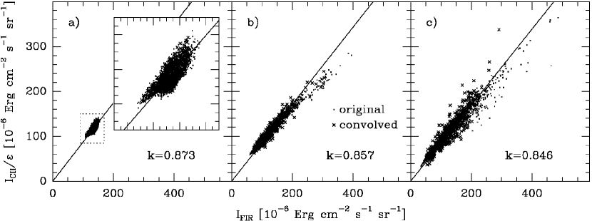
Figure 4: $I_{\rm CII}/\epsilon$ vs. $I_{\rm FIR}$ in maps calculated from the three model clouds towards the $y$–direction. The three panels, a, b and c, correspond to the three models, $A$, $B$ and $C$ respectively. The [CII] data has been convolved to a resolution of $\sim$1.2$\arcmin$ and the FIR to a resolution of $\sim 4\arcmin$. The slope of the least squares line going through the origin is given in each frame. For model $A$ the data in the indicated area has been plotted separately on a larger scale.

4.2 Efficiency of the photoelectric heating

In Fig. 4 the quantity $I_{\rm CII}/\epsilon$ is plotted versus the FIR intensity, $I_{\rm FIR}$, for the models $A$, $B$ and $C$ (left to right) observed along the $y$–direction. We show the relations for both the original data and the data convolved to the resolution of the observations discussed in Ingalls et al. (2002), that is $\sim 1.2\arcmin$ for [CII] and $\sim 4\arcmin$ for the FIR observations. The relations are close to linear, and Fig. 4 shows the least squares lines fitted to the convolved data. The range of intensities and the scatter in the relations both increase from model $A$ to model $C$. The slope of the relation decreases, albeit very slowly with increasing Mach number of the model. The fitted slopes for each of the three orthogonal directions of the lines of sight are given in Table 1.

In Sect 4.1 the [CII] intensities were found to saturate at high column densities when all incoming FUV radiation was absorbed. As a result, at high intensities the points for unconvolved data fall below the least squares line. However, at the location of intensity maxima the convolution decreases the FIR intensities more than the [CII] intensities, and in the figure the convolved points are shifted to the left more than down. This is seen especially in model $C$ that has the largest density contrast. In model $C$ the relation $I_{\rm CII}/\epsilon$ versus $I_{\rm FIR}$ for the convolved data turns slightly upwards at higher intensities, relative to the relation for the unconvolved data. In model $B$ the convolution raises the points at high-$A_{\rm V}$ only slightly closer to the fitted least squares line.

A comparison between the ratios $I_{\rm CII}/(\epsilon I_{\rm FIR})$ obtained from the models and the empirical relation $I_{\rm CII}/I_{\rm FIR}$ allows to estimate the efficiency of the photoelectric heating, $\epsilon$. In Ingalls et al. (2002) the average ratio of CII and FIR intensities is found to be $I_{\rm CII}/I_{\rm FIR}$=(2.5$\pm$0.9)$\times 10^{-2}$, for a sample of high latitude clouds observed with ISO. The slope they derive for large scale correlation using DIRBE and FIRAS observations for $|b|>5\deg$ is also very similar, $I_{\rm CII}$=(2.54$\pm$0.03)$\times 10^{-2}I_{\rm FIR}$ - (1.1365$\pm$0.0004)$\times 10^{-6}$ erg cm^-2 s^-1 sr^-1.

Table 1: The slope of the relation $I_{\rm CII}/\epsilon$ versus $I_{\rm FIR}$ in the model clouds observed from three different directions. The values are based on convolved data. The efficiency of the photoelectric heating, $\epsilon$, is obtained assuming the empirical relation $I_{\rm CII}/I_{\rm FIR}$=2.5$\times 10^{-2}$ from Ingalls et al. (2002).

Model	direction	$<I_{\rm CII}/(\epsilon I_{\rm FIR})>$	$100\times\epsilon$
A	x	0.876	2.85
A	y	0.873	2.86
A	z	0.872	2.87
B	x	0.869	2.88
B	y	0.861	2.90
B	z	0.870	2.87
C	x	0.862	2.90
C	y	0.862	2.90
C	z	0.858	2.91

We have calculated the efficiencies of the photoelectric emission, $\epsilon$, assuming $I_{\rm CII}/I_{\rm FIR}=2.5\times 10^{-2}$. The results are given in the fourth column of Table 1. We obtain an average value of $\epsilon=2.88\times 10^{-2}$. There is very little variation between the models or the direction from which the model clouds are observed. However, as seen in Fig. 1, the variation within individual maps can be quite significant. In the case of unconvolved data in Fig. 1 the variation ranges from $\sim$40% in model $A$ to almost 90% in model $C$.

5 Discussion

The observations presented by Ingalls et al. (2002) contain scatter in the plot of $I_{\rm CII}$ versus $I_{\rm FIR}$ exceeding the uncertainty of individual observations. Differences between clouds can be attributed largely to differences in the dust composition. The photoelectric heating and therefore [CII] emission depends on the abundance of very small dust grains and PAH–molecules while the far–infrared emission is caused mainly by large dust grains. The ratio between the abundances of very small grains and large grains is known to show significant spatial variations. The variations are more noticeable in dense clouds (e.g. Laureijs et al., 1991; Juvela et al., 2002; Stepnik et al., 2003), but changes have been observed even in cirrus type clouds (Bernard et al., 1999; Cambrésy et al., 2001). Variations in the radiation field are probably less important.

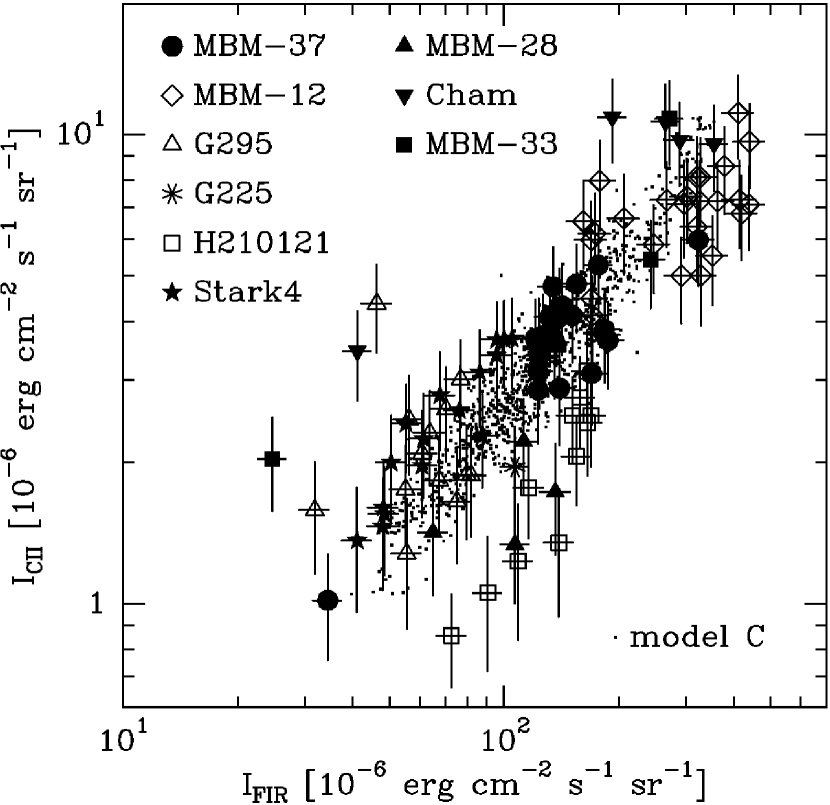
Figure 5: Comparison of the [CII] and FIR intensities in model $C$ and in the sample of HLCs in Ingalls et al. (2002). For model $C$ the points correspond to convolved data, and to an efficiency of the photoelectric heating of 2.88$\times 10^{-2}$

In the first approximation an increase in the strength of the radiation field affects FIR and [CII] intensities in the same way. However, as the increased dust temperature moves dust emission to shorter wavelengths the FIR intensity is reduced relative to the [CII] emission (FUV absorption). Assuming that the FIR intensity in the models is fixed and constrained by the observations, if the interstellar radiation field is increased the dust column density must be decreased to maintain the FIR intensity unchanged. As a result of the decreased column density, the [CII] emission is less saturated, and the ratio $I_{\rm CII}/I_{\rm FIR}$ is increased. Variations within individual clouds could similarly be caused by variations in the local radiation field or in the properties of the gas or dust.

In the present models dust properties are assumed to be constant throughout the clouds. The fractional abundance of C⁺ is also kept constant and the [CII] emission is assumed to be responsible for all of the gas cooling. Even with these simplifying assumptions the computed ($I_{\rm CII}$,$I_{\rm FIR}$) values contain a significant scatter. The scatter is smallest in the most homogeneous model $A$. Only in a completely homogeneous model the points would fall on one line as both [CII] and FIR emission would depend solely on the distance from the cloud surface. The scatter is largest in model $C$, with the largest value of $M_{\rm S}$ and density contrast. In this model, both the range of $I_{\rm CII}$ and $I_{\rm FIR}$ values and the scatter in their relation are similar to the observations presented by Ingalls et al. Such a comparison is relevant only if the observed positions were selected randomly within the clouds. This is not always the case, but the scatter of the observed points should still be close to the true variation within the observed clouds.

In Fig. 5 we compare our model $C$ with the observation presented by Ingalls et al. (2002). We have plotted in the same figure our model $C$ (direction $y$) for which the [CII] intensities have been calculated using the value $\epsilon=2.9\times 10^{-2}$ derived in Sect. 4.2. The model covers a large fraction of the observed range of $I_{\rm CII}$ and $I_{\rm FIR}$ values. After subtracting a linear fit, the remaining scatter in all observations is about twice the scatter in model $C$, even when the observational errors are taken into account. On the other hand, in individual clouds the variation is very similar to that found in the model. Our results show that most of the observed scatter may originate from the inhomogeneous density structure of the clouds, and the observed scatter is consistent with that predicted with supersonic and super–Alfvénic MHD turbulence with sonic rms Mach number $M_{\rm S}\gtrsim 2$. In subsonic models both the scatter and the total range of [CII] and FIR intensities is instead significantly smaller than in the observed clouds.

Compared with model $C$ the scatter is significantly larger only in the cloud MBM-12, which also has the highest FIR intensities. MBM-12 has an HI column density of $\sim$1.1$\times 10^{21}$ cm^-2, i.e. some 40% below the average column density of the models. Timmermann et al. (1998) suggested the cloud is subjected to stronger than average radiation field, $\chi\sim$1–2 $\chi_{0}$, and this could also explain the high FIR intensities. On the other hand, since the cloud has significant molecular line emission (Magnani et al., 1996) the total column density may not be very different from the model, and therefore the observed FIR intensities do not imply a strong radiation field by themselves. Furthermore, if one would accept the hypothesis of a strong radiation field, the low FIR colour temperature (see Ingalls et al., 2002, Fig. 4) would require a very low abundance of small dust grains.

The scatter in the observed [CII] and FIR intensities may depend on two effects not included in the models: i) CI cooling and ii) optical depth of the [CII] line. Although the models assume all the cooling is from C⁺, CI emission may be important on some lines of sight, increasing the observed scatter. According to Ingalls et al. (2002) the maximum contribution to the cooling from CI is approximately 30%. The scatter due to the the presence of CI cooling on some lines of sight should therefore be well below 15%. Furthermore, the CI contribution can be significant only for high column density, and could not explain the scatter at low FIR intensities. The models also assume that the [CII] line is optically thin. If the line became optically thick at some lines of sight, the main effect would be to flatten the $I_{\rm CII}$ vs. $I_{\rm FIR}$ relation at high column densities, while the scatter would not be significantly affected. In the models, the saturation of $I_{\rm CII}$ is caused by the total absorption of the FUV radiation that is converted into [CII] emission, not by self–absorption of the [CII] line itself. Since the observations do not show strong [CII] saturation with increasing FIR intensity, the optical depth of the [CII] line cannot be very high.

The derived value of the photoelectric heating efficiency, $\epsilon$, is close to theoretically derived values (de Jong, 1977; Bakes & Tielens, 1994). Bakes & Tielens (1994) performed theoretical calculations using a MRN type grain size distributions ($n\sim a^{-3.5}$, Mathis et al., 1977). They found that about half of the heating rate is due to grains with sizes below 15 Å  and the contribution from grains larger than 100 Å  is insignificant. The net efficiency was calculated as a function of the parameter $G_{0}(T/{\rm K})^{1/2}(n_{\rm e}/{\rm cm}^{-3})^{-1}$, where $G_{0}$ is the intensity of the far-UV radiation field relative to Habing’s field (Habing, 1968), $T$ is gas temperature and $n_{\rm e}$ the electron density. The estimated efficiency is constant $\epsilon\sim 3\times 10^{-2}$ for $G_{0}(T/{\rm K})^{1/2}(n_{\rm e}/{\rm cm}^{-3})^{-1}\lesssim 10^{3}$. This prediction should apply to the cloud sample in Ingalls et al. (2002). Bakes & Tielens found, however, that the predicted heating rate could be doubled if the exponent of the grain size distribution was decreased from -3.5 to -4.0. Since $A_{\rm V}$ and FIR intensity depend on large grains and the heating mainly on PAHs the derived efficiency $\epsilon$ is model dependent.

In this paper we have used the dust model of Li & Draine (2001). Weingartner & Draine (2001b) based their studies on the same dust model and considered further different size distributions discussed in Weingartner & Draine (2001a). For cold neutral medium ($T\sim$100 K) and size distributions consistent with the diffuse cloud extinction law, $R_{\rm V}\sim$3.1, their predictions for the photoelectric heating rate are close to the values given by Bakes & Tielens (1994). The results depend on the carbon abundance which is limited by extinction measurements to values below $\sim 6\times 10^{-5}$ carbon atoms per H nucleus (Weingartner & Draine, 2001a, b; Li & Draine, 2001). The models of Li & Draine (2001) and Weingartner & Draine (2001a) favoured carbon abundances close to this upper limit and the resulting rate of the photoelectric heating is some 25% above the value given by Bakes & Tielens (Weingartner & Draine, 2001b).

Habart et al. (2001) derived values of $\epsilon\,$=2–3% for the efficiency of the photoelectric heating across the cloud L1721. Compared with the Ingalls et al. sample, the cloud has higher visual extinction, $A_{\rm V}\sim 3^{m}$, and, due to the proximity of a B2 star, it is subjected to a stronger radiation field, $\chi\gtrsim 5\chi_{0}$. By adopting the dust model of Désert (1990), Habart et al. were able to derive efficiencies of the photoelectric emission separately for PAH, very small grain and large grain components. The derived efficiencies were $\sim 3$% for PAHs, $\sim$1% for very small grains and $\sim$0.1% for large grains. Part of the observed variation was attributed to changes in the abundance of the dust components. The clouds in the Ingalls sample have lower visual extinction, and abundance variations are expected to be correspondingly smaller.

Another source of uncertainty is the balance between the column density and the strength of the radiation field. As discussed above, if a stronger radiation field or a smaller column density were adopted in the models, the calculated ratio $I_{\rm CII}/(\epsilon\,I_{\rm FIR})$ would increase and the derived value of $\epsilon$ decrease. According to Fig. 1, the ratio $I_{\rm CII}/(\epsilon I_{\rm FIR})$ increases up to 30% above its average value when moving from the cloud center to the cloud edges, where the radiation field is not attenuated. Therefore, if the clouds had significantly lower extinction, the efficiency of the photoelectric heating could be lower by the same amount. We modified the model $C$ by reducing its column density by a factor of three and by multiplying the intensity of the external radiation field by a factor of two. The estimated average efficiency of the photoelectric heating decreased from 2.88$\times 10^{-2}$ to 2.25$\times 10^{-2}$, i.e. only by 22%. Based on HI and molecular line data the column densities are in most of the observed clouds within a factor of two from the average column density of the models. In this paper we have used for the intensity of the local ISRF values given by Mezger et al. (1982) and Mathis et al. (1983). According to Draine (1978) and Parravano et al. (2003) the actual ISRF could be up to $\sim$70% stronger. However, the difference is very unlikely to be a factor of two. The actual errors caused by the uncertainty of the column density and intensity values is therefore less than 22%.

Compared with Ingalls et al. (2002) our estimate of the photoelectric heating efficiency is smaller by one third. Most of the difference is due to a difference in the predicted FIR intensity. For example, for a model with optical depth $A_{\rm V}$=1.0 mag through the cloud Ingalls et al. obtained a 100 $\mu$m surface brightness of slightly more than 15 MJy sr^-1. For a homogeneous, spherically symmetric cloud with equal optical depth we obtain a surface brightness of $\sim$9.5 MJy sr^-1. This is close to what Bernard et al. (1992) obtained for a similar cloud model using the dust model of Désert (1990). The difference between our result and Ingalls et al. cannot be due to model geometry. One would expect more emission (higher $I_{\rm FIR}$) from a three dimensional cloud heated from all directions than from a plane parallel cloud heated on two surfaces only. The most likely explanation for the high FIR intensities obtained by Ingalls et al. (2002) is their assumption of thermal equilibrium. This means that all grains are constantly at temperatures close to 20 K and almost all absorbed energy is re-radiated in the FIR. In our case a larger fraction of the absorbed energy is radiated at shorter wavelengths because of the small particles that are temporarily heated to much higher temperatures.

6 Conclusions

We have calculated FIR emission and [CII] line emission for three–dimensional density distributions of compressible magneto–hydrodynamic turbulent flows with rms sonic Mach numbers $M_{\rm S}=$ 0.6, 2.5, and 10.0. The dust emission, $I_{\rm FIR}$, is computed with full radiative transfer calculations. The [CII] emission is estimated assuming the photoelectric heating caused by FUV photons between 0.0912$\mu$m and 0.2066$\mu$m is balanced by [CII] line emission. The FUV absorption is determined by the radiative transfer simulations, and is assumed to be equal to the [CII] line intensity divided by the unknown efficiency of the photoelectric heating, $I_{\rm CII}/\epsilon$.

The average ratio $I_{\rm CII}/(\epsilon I_{\rm FIR})$ is in all models between 0.85 and 0.88, showing that its dependence on the density contrast (Mach number) is weak. However, dense filaments are visible in the maps as regions with lower value of $I_{\rm CII}/(\epsilon I_{\rm FIR})$. The degree of correlation between $I_{\rm CII}/(\epsilon I_{\rm FIR})$ and visual extinction decreases in more inhomogeneous clouds. In the case of simulated observations convolved to different resolutions (71$\arcsec$ for [CII] and $\sim$4$\arcmin$ for FIR) most of the correlation is lost.

The scatter in the observational ($I_{\rm FIR}$,$I_{\rm CII}/\epsilon$) plot can be reproduced by models with rms Mach number $M_{\rm S}\gtrsim$2 (supersonic turbulence), showing that most of the scatter may be due to the inhomogeneous nature of the clouds (likely due to the turbulence). In subsonic models ($M_{\rm S}\lesssim$1) both the scatter and the total range of FIR and [CII] intensities become smaller than in the observed clouds. Using the empirical value $I_{\rm CII}/I_{\rm FIR}$=2.5$\times 10^{-2}$ found for high latitude clouds (Ingalls et al., 2002) the efficiency of the photoelectric heating is found to be $\epsilon\sim 2.9\times 10^{-2}$. The value is very close to the theoretical predictions for the cold neutral medium.

References

- Bakes & Tielens (1994) Bakes E.L.O., Tielens A.G.G.M., 1994, ApJ 427, 822
- Bernard et al. (1992) Bernard J.P., Boulanger F., Desert F.X., Puget J.L., 1992, A&A 263, 258
- Bernard et al. (1999) Bernard, J.-P., Abergel A., Ristorcelli I., Pajot F., Boulanger F. et al. 1999, A&A 347, 640
- Bohlin et al. (1978) Bohlin R.C., Savage B.D., Drake J.F., 1978, ApJ 224, 132
- Cambrésy et al. (2001) Cambrésy L., Boulanger F., Lagache G., Stepnik, B., 2001, A&A 375, 999
- Désert (1990) Désert F.-X., Boulanger F., Puget J. L., 1990, A&A 237, 215
- Draine (1978) Draine B.T., 1978, ApJS 36, 59
- Draine & Li (2001) Draine B.T., Li A., 2001, ApJ
- Habart et al. (2001) Habart E., Verstraete L., Boulanger F., et al., 2001, A&A 373, 702
- Habing (1968) Habing H.J., 1968, Bull. Astron. Inst. Netherlands, 19, 421
- Helou et al. (1985) Helou G., Soifer B.T., Rowan-Robinson M., 1985, ApJ 298, L7
- de Jong (1977) de Jong T., 1977, A&A 55, 137
- Ingalls et al. (2002) Ingalls J.G., Reach W.T., Bania T.M., 2002, ApJ 579, 289
- Juvela et al. (2002) Juvela M., Mattila K., Lehtinen K., et al., 2002, A&A 382, 583-599
- Juvela et al. (2003) Juvela M., Padoan P., 2003, A&A 397, 201
- Laureijs et al. (1991) Laureijs R.J., Clark F.O., Prusti T., 1991, ApJ 372, 185
- Laureijs et al. (1995) Laureijs R. J., Fukui Y., Helou, G. et al., 1995, ApJS 101, 87
- Laureijs et al. (1996) Laureijs R.J., Haikala L., Burgdorf M. et al., 1996, A&A 315, L317
- Li & Draine (2001) Li A., Draine B.T., 2001, ApJ 554, 778
- Magnani et al. (1996) Magnani L., Hartmann D., Speck B.G., 1996, ApJS 106, 447
- Mathis et al. (1977) Mathis J.S., Rumpl N., Nordsieck K.H., 1977, ApJ 217, 425
- Mathis et al. (1983) Mathis J.S., Mezger P.G., Panagia N., 1983, A&A 128, 212
- Mezger et al. (1982) Mezger P.G., Mathis J.S., Panagia N., 1982, A&A 105, 372
- Miesch et al. (1999) Miesch M.S., Scalo J., Bally J., 1999, ApJ 524, 895
- Padoan et al. (1999) Padoan P., Bally J., Billawala Y., Juvela M., Nordlund Å., 1999, ApJ 525, 318
- Padoan et al. (1997a) Padoan P., Jones B.J.T., Nordlund Å., 1997, ApJ 474, 730
- Padoan et al. (1998) Padoan P., Juvela M., Bally J., Nordlund Å., 1998, ApJ 504, 300
- Padoan et al. (2000) Padoan P., Juvela M., Bally J., Nordlund Å., 2000, ApJ 529, 259-267
- Padoan et al. (1997b) Padoan P., Nordlund Å., Jones B.J.T., 1997, MNRAS 288, 145
- Padoan & Nordlund (1999) Padoan P., Nordlund Å., 1999, ApJ 526, 279
- Parravano et al. (2003) Parravano A., Hollenbach D.J., McKee C.F., 2003, ApJ, 584, 797
- Stepnik et al. (2003) Stepnik B., Abergel A., Bernard J.-P., Boulanger F., Cambrésy L. et al. 2003, A&A 398, 551
- Timmermann et al. (1998) Timmermann R., Köster B., Stutzki J., 1998, A&A 336, L53
- Weingartner & Draine (2001a) Weingartner J.C., Draine B.T., 2001, ApJ 548, 296
- Weingartner & Draine (2001b) Weingartner J.C., Draine B.T., 2001, ApJS 134, 263
- Wolfire et al. (1995) Wolfire M.G., Hollenbach D., McKee C.F., Tielens A.G.G.M., Bakes E.L.O., 1995, ApJ 443, 152