The Quintuple Quasar: Radio and Optical Observations

Abstract

We present results from high-resolution radio and optical observations of PMN J0134–0931, a gravitational lens with a unique radio morphology and an extremely red optical counterpart. Our data support the theory of Keeton & Winn (2003): five of the six observed radio components are multiple images of a single quasar, produced by a pair of lens galaxies. Multi-frequency VLBA maps show that the sixth and faintest component has a different radio spectrum than the others, confirming that it represents a second component of the background source rather than a sixth image. The lens models predict that there should be additional faint images of this second source component, and we find evidence for one of the predicted images. The previously-observed large angular sizes of two of the five bright components are not intrinsic (which would have excluded the possibility that they are lensed images), but are instead due to scatter broadening. Both the extended radio emission observed at low frequencies, and the intrinsic image shapes observed at high frequencies, can be explained by the lens models. The pair of lens galaxies is marginally detected in HST images. The differential extinction of the quasar images suggests that the extreme red color of the quasar is at least partly due to dust in the lens galaxies.

1 Introduction

The quasar PMN J0134–0931 calls attention to itself in many ways. It is very bright at radio frequencies (1 Jy at 2 GHz); its optical counterpart is extraordinarily red ($B-K\geq 11$); and it has a unique radio morphology consisting of six compact components within a circle of diameter $0\farcs 7$. It is therefore unsurprising, in retrospect, that it was discovered to be an interesting object by two independent groups.

Winn et al. (2002a; hereafter, W02) found it during a survey for radio-loud gravitational lenses. They showed that at least five of the six radio components have identical continuum radio spectra, and discovered a curved arc of radio emission joining two of the components. These properties are hallmarks of strong gravitational lensing.

Gregg et al. (2002; hereafter, G02) found it in a cross-compilation of radio, optical, and near-infrared catalogs that was designed to identify the reddest quasars on the sky. They measured its redshift ($z_{s}=2.2$) and found at least three components in a near-infrared image. The multiplicity of the near-infrared counterpart, and the extremely large inferred luminosity ($M_{R}=-29.6$, even under the conservative assumption of no extinction) were evidence of gravitational lensing.

However, neither group could explain the unique morphology with a plausible lens model, because strong lensing by a single galaxy usually results in only two or four images. Another difficulty was that two of the components were found to have a lower surface brightness than the other components in high-resolution radio images, in apparent contradiction of the conservation of surface brightness by gravitational lensing.

Also unknown was the reason for the extremely red color of J0134–0931. The two most obvious possibilities—reddening due to dust in the host galaxy, or due to dust in the lens galaxy—could not be distinguished. Hall et al. (2002) detected strong Ca II H and K absorption lines at $z_{l}=0.76$ (presumably the lens redshift), but they were not able to determine the reason for the redness of the quasar spectrum.

In a companion paper, Keeton & Winn (2003; hereafter, KW03) present the first quantitative models that explain all the previously known properties of J0134–0931. In those models, five of the radio components are multiple images of a single quasar, and the sixth component represents a different source, which is presumably a second component of the same background radio source. The positions of the two lens galaxies are constrained remarkably well by the observed image configuration. Furthermore, the two low-surface-brightness components are located close to the expected position of one of the lens galaxies, suggesting that scatter broadening by ionized material in that lens galaxy could account for their large angular sizes.

In addition to explaining the previous data, the KW03 models make a number of predictions about more subtle properties of J0134–0931 that would be detectable in radio and optical observations with high sensitivity and high angular resolution. In this paper we present multi-frequency observations of J0134–0931 with the Very Long Baseline Array (VLBA) and the Hubble Space Telescope (HST) that confirm some of these predictions, and refute none of them.

Before describing the new observations, in § 2 we provide an overview of the previously-known radio morphology of J0134–0931, and the nomenclature used to describe it. We also review the main features of the KW03 models. The radio data (§ 3) confirm that the sixth and faintest radio component has a significantly different spectral index than the other five components (§ 3.3). The two components that were observed to have larger angular sizes are indeed being scatter broadened (§ 3.4). There is tantalizing (but tentative) evidence for one of the additional images of the second background source that are predicted by the KW03 models (§ 3.5). The extended radio emission (§ 3.6) and component shapes (§ 3.7) can be explained by the models.

After subtracting point sources from the optical images (§ 4.1), we identify two faint but significant peaks of residual flux as direct detections of the lens galaxies (§ 4.2). The optical counterparts of the radio components have different colors, and their optical flux ratios differ from their radio flux ratios, implying that the extreme red color of J0134–0931 is at least partly due to reddening by dust in the lens galaxy (§ 4.3). Finally, in § 5, we summarize the evidence that J0134–0931 is the first known instance of a quintuply-imaged quasar.

2 Overview

Figure 1 is a diagram of the observed configuration of the radio components. The dots represent the six compact radio components A–F, which are named in decreasing order of radio flux density. The size of each dot is proportional to the logarithm of its flux density ratio relative to component D. The angular sizes of C and E are much larger than the other components at 1.7 GHz and 5.0 GHz, which is why we have used gray dots to represent those components instead of black dots. There is a curved arc extending between A and B at 1.7 GHz, represented schematically by a solid line. Components A–E all have the same spectral index, as measured from 5 GHz to 43 GHz ($\alpha=-0.69\pm 0.04$, where $S_{\nu}\propto\nu^{\alpha}$), but the spectral index of F was unknown.

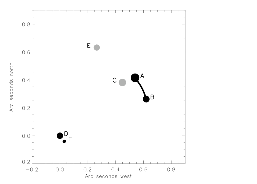
Figure 1: Illustration of the morphology of J0134–0931.

According to the KW03 models, the background radio source has two components (S₁ and S₂) and there are two lens galaxies (Gal-N and Gal-S). The five observed radio components A–E are five images of S₁, and F is the brightest of three images of S₂. The positions and masses of the lens galaxies are fairly well constrained by the data, but their ellipticities and position angles are not. For reference, the critical curves and caustics of a representative lens model are shown in Fig. 2. The reader is referred to KW03 for a full theoretical analysis.

Figure 2: Representative lens model of J0134–0931, from KW03. Left: source plane, with caustics (solid lines), source component S₁ (black dot), and source component S₂ (black square). The image multiplicity of each region is reported as $N_{\rm tot}/N_{\rm bri}$, where $N_{\rm tot}$ is the total number of images, and $N_{\rm bri}$ is the number of bright (non-core) images. Right: image plane, with critical curves (solid lines), images of S₁ (black dots), and images of S₂ (black squares).

3 Radio evidence

3.1 Observations and calibration

This system was observed with the VLBA at 1.7 GHz and 5.0 GHz by W02. Below, we present the results from new VLBA observations at three different frequencies. We also present images based on both the old and the new data, to provide a uniform multi-frequency study. A list of the basic parameters of all the VLBA observations is given in Table 1.

The new observations were conducted in standard VLBA continuum frequency bands at 2.3 GHz, 8.4 GHz, and 15 GHz. The array consisted of the usual ten antennas, except that the Pie Town antenna did not participate in the 15 GHz observation. For the 2.3 GHz observation, we did not employ phase referencing because the source was sufficiently bright for self-calibration. At the higher frequencies, we switched between J0134–0931 and the nearby, bright, compact source J0141–0928 in order to calibrate the relative antenna gains. The cycle times were 4 minutes and 2 minutes at 8.4 GHz and 15 GHz, respectively. Short observations of the bright radio sources J2253+1608 and J0555+3948 were included to serve as fringe-finders and to correct large delay errors.

The observing bandwidth of 32 MHz per polarization was divided into 4 sub-bands of width 8 MHz. Both senses of polarization were recorded with 1-bit sampling. The data were correlated in Socorro, New Mexico, producing 16 channels of width 0.5 MHz from each sub-band, with an integration time of one second.

Calibration was performed with aips using standard procedures summarized as follows. Obviously corrupted data, and data taken at elevations less than $15\arcdeg$, were discarded. Visibility amplitudes were calibrated using on-line measurements of antenna gains, system temperatures, and voltage offsets in the samplers. Large delay errors were removed by fringe-fitting the data from a 1.5-minute observation of J2253+1608 and applying the delay corrections to all the data. At 2.3 GHz, we corrected residual rates, delays, and phases by fringe-fitting the data from J0134–0931 directly; at the higher frequencies we fringe-fitted data from J0141–0928 and interpolated the solutions. After calibration, the data were averaged in time and frequency in order to reduce the data volume, but we ensured that the final sampling was still fine enough to produce $<$1% smearing over the desired field of view.

Table 1: Observations of J0134–0931 with the VLBA.

Start Date	Frequency	Duration	Field size	Pixel scale	Beam parameters		R.M.S. noise
(UT)	(GHz)	(hours)	($N_{\rm pix}\times N_{\rm pix}$)	(mas pixel-1)	$b_{\rm maj}\times b_{\rm min}$ (mas)	P.A. (degrees)	(mJy beam-1)
2000 Apr 28	4.99	1	$2048\times 2048$	0.50	$6.5\times 3.5$	$12\fdg 7$	0.30
2000 Oct 31	1.67	4	$1024\times 1024$	1.00	$17.1\times 4.9$	$19\fdg 1$	0.20
2001 Oct 17	2.27	7	$1024\times 1024$	1.00	$10.1\times 3.8$	$-3\fdg 0$	0.23
2001 Dec 08	8.42	7	$4096\times 4096$	0.25	$4.3\times 2.3$	$9\fdg 8$	0.13
2002 Feb 02	15.36	7	ABC: $2048\times 2048$	0.15	$1.5\times 0.5$	$-6\fdg 3$	0.36
			DF: $1024\times 0.15$	0.15	$1.5\times 0.5$	$-6\fdg 3$	0.32
			E: $1024\times 0.15$	0.15	$1.5\times 0.5$	$-6\fdg 3$	0.37

3.2 Images and general results

Imaging was performed with aips. For each frequency, we first applied a Gaussian tapering function to the visibility data, to emphasize the low-resolution (short-baseline) information, and used the clean algorithm to create a preliminary model of the detected radio structures. This model was used to self-calibrate the antenna phases. A new map was created with no tapering function, and the process of cleaning and self-calibration was repeated until no further improvement was noted. We then used the latest clean model to self-calibrate the relative amplitudes of the antennas with a solution interval of 30 minutes. The amplitude corrections were typically smaller than 10%. We used a moderately uniform weighting (robust $=0$, in aips) for the final images.

We also applied the self-calibration and imaging procedures described above to the previously published 1.7 GHz and 5.0 GHz data, for the sake of uniformity. This resulted in an improvement in dynamic range over the previously published images, due to the increased care in removing corrupted data, the use of amplitude self-calibration, and the different choice of visibility weighting.

In all cases except 15 GHz, we created one wide-field image, centered between components B and D in right ascension, and between D and E in declination. At 15 GHz we used the multiple-field clean algorithm to deconvolve three fields simultaneously: one field centered on components A, B, and C; one field centered on component E; and one field centered on components D and F.

Figure 3 shows wide-field grayscale images for all frequencies except 15 GHz. These images provide an overview of the detected radio structures. To ease the visual interpretation of these images, they were created after applying a Gaussian tapering function to the visibility data, and were restored with a circular Gaussian beam. For the 1.7 GHz and 2.3 GHz images, the tapering function declined to 30% at a visibility radius of $10^{6}\lambda$, and the restoring beam had a diameter of 20 milli-arc seconds (mas). For the 5.0 GHz and 8.4 GHz images, the corresponding values were $3\times 10^{6}\lambda$ and 7 mas.

We also present narrow-field contour maps of the fields surrounding components A, B, and C (Figure 4), components D and F (Figure 5), and component E (Figure 6). The 15 GHz contour maps are presented separately for each component (Figure 7). All the contour maps were created without any tapering function and therefore employ the full resolution of the observations. These contour maps allow for a closer examination of individual component sizes and shapes. The most important parameters describing these full-resolution images are given in Table 1: the image dimensions, the major and minor axes (full-width-half-maximum) and orientation of the restoring beam, and the root-mean-squared (R.M.S.) noise level.

We draw attention to some features of these images and contour maps that will be discussed in detail, and placed in the context of the KW03 models, in subsequent sections:

1. Component F is detected at all frequencies except 15 GHz. It is especially prominent at 1.7 GHz but fades relative to D as the frequency increases (§ 3.3).

2. Components C and E are heavily resolved at 1.7 GHz, are faint and resolved at 2.3 GHz and 5 GHz, and are compact and bright at the highest frequencies. By contrast, components B and D are compact at all frequencies (§ 3.4).

3. In the 1.7 GHz map, there is extended radio emission near the expected location of C, but its centroid appears to be shifted $\approx$30 mas south (§ 3.5).

4. The radio arc between A and B was detected at the two lowest frequencies. In addition, at 1.7 GHz, there is a significant extension of component A towards the expected location of C (§ 3.6).

5. At 15 GHz (Fig. 7), component B appears to be a fainter and parity-reversed copy of component A. Component C is elongated along a line pointing to A (§ 3.6).

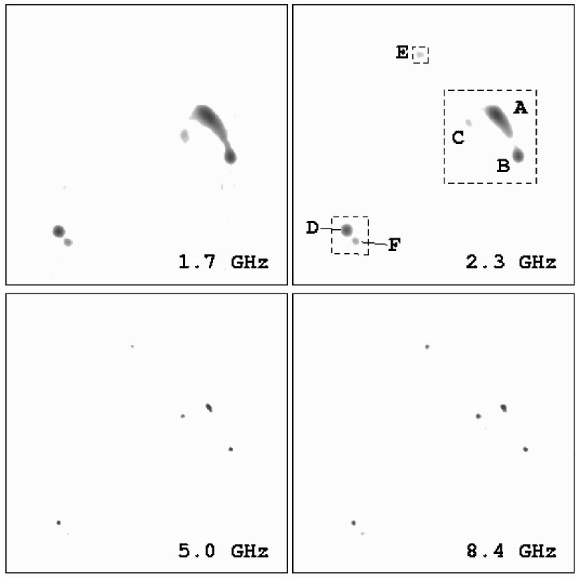
Figure 3: Grayscale VLBA images ($1\arcsec\times 1\arcsec$) at four frequencies. The first gray level has been set to $8\sigma$, where $\sigma$ is the R.M.S. noise level given in Table 1. North is up and east is left. In the upper right panel, A–F are labeled, and dashed lines indicate the regions shown at full resolution for 1.7–8.4 GHz in Figs. 4–6.

Figure 4: Radio contour maps of the $0\farcs 24\times 0\farcs 24$ field surrounding components A, B, and C. Contours begin at $3\sigma$ and increase by factors of 2, where $\sigma$ is the R.M.S. noise level. The restoring beam is illustrated in the lower left corner of each panel. In the upper left panel (1.7 GHz), black dots mark the positions of A, B, and C (as measured at higher frequencies) and the predicted position of ${\rm C}^{\prime}$.

Figure 5: Radio contour maps of the $0\farcs 12\times 0\farcs 12$ field surrounding components D and F. Contours begin at $3\sigma$ and increase by factors of 2, where $\sigma$ is the R.M.S. noise level. The restoring beam is illustrated in the lower left corner of each panel.

Figure 6: Radio contour maps of the $0\farcs 04\times 0\farcs 04$ field surrounding component E. Contours begin at $3\sigma$ and increase by factors of 2, where $\sigma$ is the R.M.S. noise level. The restoring beam is illustrated in the lower left corner of each panel.

Figure 7: 15 GHz contour maps of the $0\farcs 008\times 0\farcs 008$ field surrounding each of components A–F. Contours begin at $3\sigma$ and increase by factors of 2, where $\sigma=0.35$ mJy beam^-1 is the R.M.S. noise level. The restoring beam is illustrated in the lower left corner of each panel.

3.3 Component F

We measured the total flux density of each radio component by fitting an elliptical Gaussian function to the appropriate region of each VLBA image using the aips procedure jmfit, which takes into account the ellipticity of the restoring beam. The results are given in Table 2. The flux densities of components A, B, D, and F are plotted in Figure 8 as a function of frequency. Also plotted is the total flux density of all components, from the measurements compiled by W02. The upper limit on the flux of F at 15 GHz represents the $3\sigma$ level in that region of the image. Results for components C and E are not plotted because, for these components, a substantial amount of flux is “resolved out” at low frequencies due to the interferometer’s lack of short baselines.

The continuum spectra of components A, B, and D are nearly identical, while the spectrum for component F is significantly steeper. To make the difference in spectral slope obvious to the eye, we have divided the flux densities of D by 9, to match the 1.7 GHz flux density of F, and plotted the results with open squares. Using the measurements at which the components are fairly compact and the fitting results are therefore most accurate, we find spectral slopes of $\alpha_{\rm A}=-0.64\pm 0.08$, $\alpha_{\rm B}=-0.65\pm 0.07$, and $\alpha_{\rm D}=-0.63\pm 0.07$ (where $S_{\nu}\propto\nu^{\alpha}$). These values agree with the value $\alpha=-0.69\pm 0.04$ measured by W02 using lower-resolution data. For component F, using measurements at all frequencies for which it was detected, $\alpha_{\rm F}=-1.07\pm 0.13$.

In the KW03 scenario, A–E are multiple images of the same quasar, and should have nearly identical spectral indices, but F need not have (and probably would not have) the same spectral index. It was already established by W02 that A–E have the same spectral index. By establishing that F has a different spectral index than the other components, our analysis has confirmed this key expectation of the KW03 models.

Table 2: Total radio flux densities

Component	Total flux density (mJy)
	1.7 GHz	2.3 GHz	5.0 GHz	8.4 GHz	15 GHz
A	$\mathit{420\pm 20}$	$\mathit{530\pm 30}$	$309\pm 1$	$242.4\pm 0.3$	$143\pm 1$
B	$\mathit{144\pm 7}$	$\mathit{133\pm 7}$	$78.4\pm 0.6$	$56.2\pm 0.3$	$35\pm 1$
C	$\cdots$	$\cdots$	$18\pm 1$	$41.4\pm 0.6$	$28\pm 2$
D	$98.5\pm 0.4$	$98.5\pm 0.5$	$60.6\pm 0.6$	$43.8\pm 0.3$	$26.0\pm 0.7$
E	$\cdots$	$\cdots$	$8\pm 1$	$12.3\pm 0.3$	$12\pm 1$
F	$11\pm 1$	$9\pm 1$	$5\pm 1$	$1.8\pm 0.3$	$<0.96$ ($3\sigma$)

Note. — Flux densities estimated from elliptical Gaussian fits to the radio components. Italics indicate cases for which this approximation is especially poor. Entries for C and E are not given for cases where the components were almost completely resolved out.

Figure 8: Flux densities of components A, B, D, and F. Where not shown as error bars, the statistical errors are comparable to the symbol sizes, or smaller. Also plotted are the measurements of the total flux density of all components, compiled by W02 from various sources.

3.4 Scatter broadening

One objection to the KW03 models, or any scenario in which components A–E are gravitationally lensed images of a single source component, is that components C and E were observed to have a much lower surface brightness at 1.7 GHz and 5.0 GHz than the other components. The problem is that gravitational lensing cannot alter surface brightness. However, it is possible for a non-gravitational effect, namely scatter broadening due to electron-density fluctuations in the lens galaxy or our own Galaxy, to cause differences in the surface brightness of lensed images. If different images pass through different electron columns they will be broadened by different amounts.

Scatter broadening can be recognized because the angular size of an affected source increases strongly with observing wavelength. For a source that is intrinsically a point source, the angular size due to scatter broadening is typically proportional to $\lambda^{n}$ where $n\approx 2$ (for a review, see Rickett, 1990). A particularly well-studied case is Sgr A^∗ (see, e.g., Jauncey et al., 1989; Lo et al., 1993; Doeleman et al., 2001). Among gravitational lenses, the best-studied case of differential scatter broadening is PKS 1830–211 (Jones et al., 1996; Guirado et al., 1999). In that case, the broader image passes through the spiral arm of the lens galaxy where a higher electron column density might be expected (Winn et al., 2002b; Courbin et al., 2002).

Our VLBA maps strongly suggest that components A, C, and E are being scatter broadened. All three of these components are fairly compact at 15 GHz, but are heavily resolved at 5 GHz and very heavily resolved at 1.7 GHz. This is despite the decreasing angular resolution of the observations as one proceeds to lower frequencies. To test the $\lambda^{2}$-dependence, we fitted elliptical Gaussians to all the components detected in each image (as in § 3.3). The fitting procedure takes into account the intrinsic ellipticity of the beam and finds the deconvolved major and minor axes ($b_{\rm maj}$ and $b_{\rm min}$). We note that it would be preferable to fit models to the visibility data rather than the image data, because the noise properties of the visibility data are better understood, but in this case visibility-fitting was unfeasible because of the large data volume. We also note that not all the components are well described by ellipses, especially at 15 GHz, but the results from elliptical fits should be accurate enough to determine the approximate logarithmic scaling.

Figure 9 shows the dependence of $b_{\rm maj}$ on $\lambda$ for components A, C, and E. As a measure of the angular resolution, we have plotted black dots indicating the length of the minor axis of the restoring beam, which is approximately proportional to $\lambda$. For comparison, we have also plotted the results for component D, which does not exhibit scatter broadening; its size is comparable to or smaller than the beam minor axis in all cases except 1.7 GHz. (Component B does not appear to be scatter-broadened either, but the results are not plotted in order to reduce clutter.)

Components A, C, and E are well-approximated by the $\lambda^{2}$ law (dashed line), although the true dependence is not as steep, especially when the 15 GHz (2 cm) point is included. Given that scatter broadening seems inevitable as an explanation for the wavelength-dependent morphology of these components, we believe that the departure from the $\lambda^{2}$ law shows that the observed angular size is partially intrinsic at the shortest wavelengths. The dotted line shows the expectation of a scatter-broadened source with intrinsic size 2 mas. The source shapes in the 8.4 GHz and 15 GHz images appear to be mainly intrinsic. The flux densities, major and minor axis sizes, and position angles of the components, taken from the 15 GHz image in order to minimize scatter broadening, are given in Table 3.

The observed angular sizes can be used to estimate the scattering measure (SM) along the lines of sight to the broadened components. The SM is defined as the line-of-sight integral of $C_{n}^{2}$, where $C_{n}^{2}$ is the normalization of the power spectrum of electron-density fluctuations. Assuming a Kolmogorov spectrum, the SM can be related to the observed broadening of an extragalactic source via the relation (see Fey, Spangler, & Cordes 1991, Eq. 4; or Cordes & Lazio 2003, Eq. A17):

$${\rm SM}=\left(\frac{\theta_{\rm FWHM}}{\rm 130~{}mas}\right)^{5/3}\left(\frac{\nu}{\rm 1~{}GHz}\right)^{11/3},$$ (1)

where $\nu$ is the frequency at the lens redshift, and SM has the units m^-20/3 kpc. This predicts that angular size should vary as $\lambda^{2.2}$, a little steeper than observed. Nevertheless, the best fit to the data plotted in Fig. 9 gives SM $\approx$ 15–25 m^-20/3 kpc. This value is too large to be attributed to ionized material in our Galaxy. The Galactic latitude of J0134–0931 is $-70\arcdeg$, and the SM along such high-latitude lines of sight in the Galaxy is typically less than $10^{-3}$ m^-20/3 kpc (Cordes & Lazio 2003, Fig. 6).

By contrast, the SM for low-latitude lines of sight in our Galaxy can exceed $10^{3}$ m^-20/3 kpc, and has an average value of order unity within $|b|<5\arcdeg$. This suggests that a spiral lens galaxy viewed nearly edge-on could produce the observed broadening, although it seems unlikely that the disk would be aligned just right to intersect all three components A, C, and E. It could also be that the lens galaxy has a larger electron content than our Galaxy. We caution, however, that comparisons with our Galaxy may be misleading because the observed major axes of $\approx$30 mas at 18 cm correspond to a physical size of $\approx$150$h^{-1}$ pc at the lens redshift, which is much larger than the length scales probed by scattering effects in our Galaxy. (For exactly that reason, observations of scatter broadening in gravitational lens systems such as J0134–0931 may prove useful for characterizing electron-density fluctuations on scales inaccessible in our Galaxy.)

Table 3: Radio component shapes at 15 GHz

Component	Peak flux density	Total flux density	Major axis	Minor axis	Position angle
	(mJy beam-1)	(mJy)	(mas)	(mas)	($\arcdeg$ E of N)
A	$43.9\pm 0.4$	$143\pm 2$	$2.24\pm 0.02$	$0.48\pm 0.03$	$23.5\pm 0.5$
B	$13.6\pm 0.4$	$35\pm 1$	$2.2\pm 0.1$	$0.1\pm 0.1$	$20\pm 2$
C	$5.1\pm 0.3$	$28\pm 2$	$2.4\pm 0.2$	$0.8\pm 0.3$	$100\pm 6$
D	$18.8\pm 0.3$	$26\pm 1$	$0.93\pm 0.06$	$0.2\pm 0.1$	$14\pm 4$
E	$3.7\pm 0.3$	$12\pm 1$	$1.6\pm 0.3$	$1.0\pm 0.2$	$10\pm 20$

Figure 9: Deconvolved major axes of components A, C, D, and E, as measured from elliptical Gaussian fits to the VLBA images. Black dots indicate the size of the minor axis of the restoring beam. The dashed line is the trend expected for a scatter-broadened point source; the dotted line is for a source with intrinsic size 2 mas.

3.5 Counter-images of component F

Component F, in the KW03 models, is actually the brightest of three images of the second source component S₂. The other two images of S₂ (the “counter-images” of F) are expected to be located just south of components C and E. For convenience, we refer to the hypothetical counter-images near C and E as components ${\rm C}^{\prime}$ and ${\rm E}^{\prime}$, respectively. The KW03 models suggest that the flux ordering, from brightest to faintest, is F–${\rm C}^{\prime}$–${\rm E}^{\prime}$. It is also possible that there are two additional counter-images located between A and B, for a total of five, but the models that produce these two additional counter-images occupy a tiny volume in the phase space of model parameters explored by KW03.

There is suggestive evidence for one of these counter-images in the 1.7 GHz map. In Fig. 4, black dots mark the positions of A, B, and C (as measured at higher frequencies), and the predicted position of ${\rm C}^{\prime}$. There is a puff of extended radio emission located $\approx$30 mas due south of the expected position of component C. The location of the peak emission is not consistent with C, but it is within 6 mas of the predicted position of ${\rm C}^{\prime}$. Its total flux density is $\approx$10 mJy, or $\approx$90% of the total flux density of F, which is also the expectation of the KW03 models.

It is therefore possible that C is almost completely resolved out at 1.7 GHz, and the extended emission that is observed is instead the scatter-broadened counter-image ${\rm C}^{\prime}$. The reason we consider the evidence “suggestive” rather than definitive is that ${\rm C}^{\prime}$ was not detected at any other frequency. In particular, the 8.4 GHz data are inconsistent with $S_{{\rm C}^{\prime}}/S_{\rm F}=0.9$, unless ${\rm C}^{\prime}$ is being scatter-broadened even at that higher frequency. Therefore, we withhold final judgment on whether the detected flux is actually ${\rm C}^{\prime}$ until it can be detected at a higher frequency. The challenge will be to achieve the required signal-to-noise ratio in spite of the steep spectrum of S₂ (see § 3.3).

Assuming that we did not detect additional radio components, we can set upper limits on the fluxes on ${\rm C}^{\prime}$ and ${\rm E}^{\prime}$. We express these limits as ratios relative to component F, because lens models directly prescribe the magnification ratios of the counter-images relative to component F. We derive the limits from the 8.4 GHz map, because that is the highest-frequency image in which F is detected. By requiring the flux density of a point source be below $5\sigma$, where $\sigma$ is the noise level of the 8.4 GHz image, we find $S_{{\rm C}^{\prime}}/S_{\rm F}<0.57$ and $S_{{\rm E}^{\prime}}/S_{\rm F}<0.57$.

As discussed in detail by KW03, the limit on ${\rm E}^{\prime}$ is not constraining, but the limit on ${\rm C}^{\prime}$ formally rules out all but a few models. However, as mentioned previously, the true limit on ${\rm C}^{\prime}$ may be weaker due to scatter broadening. For example, assuming that the observed sizes of C and E at 8.4 GHz are due entirely to scatter broadening, we might allow ${\rm C}^{\prime}$ and ${\rm E}^{\prime}$ to have the same ratio of total to peak flux density. Modified in this way, the upper limits become $S_{{\rm C}^{\prime}}/S_{\rm F}<2.1$ and $S_{{\rm E}^{\prime}}/S_{\rm F}<1.1$, which are consistent with all the KW03 models. The truth lies somewhere between these extremes, because the observed sizes of C and E at 8.4 GHz are probably at least partially intrinsic (see § 3.4).

3.6 Extended emission

The radio arc joining components A and B was known previously, and is a natural consequence of the KW03 models. In addition, the KW03 models predict there should be a bridge of radio emission between components A and C. The detailed surface brightness profile of the bridge depends on the source size and shape, but it is otherwise a robust prediction.

There are two indications in the radio maps that this is correct. The first indication is found in the lowest-frequency (1.7 GHz) image, in which there are faint traces of extended flux between components A and C. This can be seen in the upper left panel of Fig. 3, as a faint prong extending eastward from component A, but is more easily seen in the upper left panel of Fig. 4. The lowest 3 contours ($3\sigma$, $6\sigma$, and $12\sigma$) bulge eastward from A to C.

The second indication is the orientation of component C in the higher-frequency (5 GHz, 8.4 GHz and 15 GHz) images. The deconvolved position angle of C is oriented nearly along the direction to component A. For example, at 15 GHz, where we expect the observed orientation to be intrinsic, component C is elongated with position angle $100\arcdeg\pm 6\arcdeg$, whereas the direction from C to A has position angle $110\arcdeg$ (see the lower left panel of Figure 4).

3.7 Component shapes

Since we have argued that the observed sizes of the radio components at 15 GHz are mainly intrinsic, the morphologies of the components should provide clues about the properties of the background source and the correct lens model. In Fig. 7, component A appears to be a two-sided core-jet source. There is a longer and more prominent jet directed southwest of the core, towards B, and there is a shorter jet directed northeast. Component B also appears to be a core-jet source, but only one jet is observed, and is directed northeast, towards A. Apparently, A and B are opposite-parity images of a two-sided core-jet source, but only one jet is apparent in B due to the relative compression of that image by the lens mapping.

The morphologies of the other components are simpler. Component C is highly elongated towards A, as already noted. Component D is mainly compact but does have a faint extension to the southwest, suggesting that D and A have the same parity. Component E is resolved but is too faint for a detailed examination. Component F was not detected.

The KW03 models predict that A and B have opposite parities, and that A and D have the same parity, which is consistent with the observed morphologies. In addition, the position angles given in Table 3 for components A–E can be produced by 23% of the models discussed by KW03. However, we caution against over-interpreting the shape parameters. As described in § 3.4, they were derived by the simple procedure of fitting a single elliptical Gaussian function to each component. The quoted errors are the statistical errors in the fitting process, and are therefore under-estimated for those components that are not well described by ellipses (especially A and B). The most secure parameters are the position angles, and the least secure parameters are the minor axis lengths (which in some cases are considerably smaller than the restoring beam).

4 Optical evidence

4.1 Observations and data reduction

On 2001 July 18 we obtained optical images of J0134–0931 in the F555W (hereafter, $V$) and F814W ($I$) filters on the WFPC2 camera of the HST. We obtained two 21.7-minute exposures at each of two dither positions, for a total exposure time of 86.8 minutes per filter. The target was centered in the PC chip, which has a pixel scale of $0\farcs 0456$ pixel^-1. The exposures were combined and cosmic rays rejected using standard iraf procedures. The images are shown in the upper two panels of Figure 10. Components A and B were detected in both filters. Component D was detected in $I$-band but is nearly absent in $V$-band.

These same data were previously analyzed by Hall et al. (2002), who also measured the optical flux ratios and detected residual flux after subtracting point sources at the positions of the radio components. Our results confirm this previous work. However, as described below, our more detailed methods have allowed us to proceed further in the interpretation of the results.

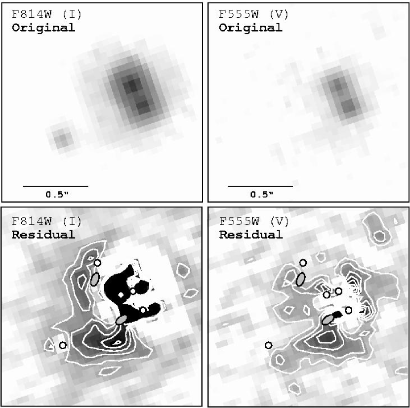
Figure 10: HST images of J0134–0931. North is up and east is left. In the residual images (bottom), the positions of the subtracted components A–E are marked by white circles. The small gray ellipses indicate the approximate range of lens galaxy positions predicted by KW03.

4.2 Detection of the lens galaxies

We built photometric models of the HST images using custom software for convolving a parametric model with a simulated PSF and varying the model parameters to achieve the best fit to the images. The simulated PSF was generated with the Tiny Tim program by Krist & Hook (1997). For the $V$-band image, the model consisted of 5 point sources, representing the radio components A–E. At $I$-band we found that components A and B are not well represented by point sources, possibly due to a contribution from the quasar host galaxy. We obtained much smaller residuals by allowing for small Gaussian components at the locations of both A and B, in addition to point sources.

Even with this modification, there were still significant residuals. In Figure 10 we show the residuals as grayscale images overlaid with white contours. The positions of the subtracted components are marked with white circles. The ring of negative residuals surrounding component A is spurious and due to imperfect PSF subtraction, but there are two peaks of positive emission in the residual images.

1. The “northern peak,” $0\farcs 14$ south and $0\farcs 12$ east of E, and

2. The “southern peak,” $0\farcs 37$ south and $0\farcs 03$ east of C.

We believe these two peaks represent genuine emission rather than artifacts of the subtraction. This pattern of residuals did not appear when we applied the same fitting and subtraction procedure to an isolated field star on the PC chip. In addition, although the peaks are more prominent in $I$-band, they are detected in both filters, despite the completely different PSF.

Hall et al. (2002) already noted the presence of low-surface-brightness flux underlying the point sources. However, the pattern in their residual image is less obvious, possibly due to an inferior PSF subtraction. They used only integral pixel shifts, did not simultaneously fit for the fluxes of the point sources, and did not allow for any extension of A and B.

Interestingly, G02 also found two residual peaks of emission by deconvolving a ground-based $K^{\prime}$-band image. The locations of each $K^{\prime}$-band peak is within $0\farcs 2$ of the corresponding peak in our images, which is fairly good agreement, considering that the spurious residuals around A may be corrupting our measurements of the peak locations. Although G02 were unsure whether the $K^{\prime}$-band peaks represented genuine emission, or artifacts of the deconvolution, we argue that the observation of similar peaks at both $I$-band and $V$-band lends confidence to all three detections.

The detection of two diffuse light sources is a further confirmation of the two-galaxy KW03 lens models. As discussed further by KW03, the predicted positions of the galaxies are both within $0\farcs 15$ of the observed locations at $I$-band and $V$-band. The approximate range of lens galaxy positions predicted by KW03 is indicated by the two small gray ellipses in Figure 10.

It is not clear how seriously to take the observed morphologies of the northern and southern peaks, because they are faint, and because of possible contamination by spurious residuals from the PSF subtraction. Nevertheless, given the morphology of the southern peak observed in both filters, we conjecture that the southern lens galaxy is elongated east-west, and overlaps component D at its easternmost extent. This would explain the very red color of D (see § 4.3).

4.3 Photometry and colors of the components

We measured the optical fluxes of components A–E using the PSF-fitting procedure described above. The optical flux ratios for A–E, relative to component B, are given in Table 4 for both the $I$ and $V$ filters. For some components we could derive only upper limits. For reference, we also list the radio values measured by W02.

Table 4: Flux ratios relative to component B

Component	F555W$\approx V$	F814W$\approx I$	Radio
A	$0.86\pm 0.05$	$1.65\pm 0.09$	$4.1\pm 0.2$
B	$1.00$	$1.00$	$1.00$
C	$<0.18$	$<0.18$	$0.87\pm 0.05$
D	$<0.011$	$0.045\pm 0.003$	$0.76\pm 0.03$
E	$<0.017$	$<0.004$	$0.24\pm 0.01$

To convert the fluxes to standard photometric magnitudes, we adopted zero points of 21.69 for F814W and 22.56 for F555W, based on the work of Dolphin (2000) and corrected for infinite aperture. No correction was attempted for the charge-transfer-efficiency (CTE) problem of WFPC2. The total magnitudes of all the components in our model was $I=18.84\pm 0.05$ and $V=22.54\pm 0.07$, in good agreement with the ground-based photometry of W02 ($I=18.79\pm 0.05$, $V=22.47\pm 0.09$).

All the components that were detected are very red. Even component B, the bluest of the detected components, has $V-I=3.4$. This is redder, for example, than any of the 157 quasars in the radio-selected (and optically unbiased) sample of Parkes sources that was investigated by Francis, Whiting, & Webster (2000) (see Fig. 4 of that work).

The optical flux ratios disagree strongly with the radio flux ratios, even though gravitational lensing is achromatic. This is a common observation among gravitational lenses, usually attributed to dust extinction by the lens galaxy (see, e.g., Falco et al., 1999) or optical microlensing (Wambsganss & Paczynski, 1991), although in this case the differential extinction is larger than usual. By comparing the radio flux ratios and the optical flux ratios, we can estimate the difference between the $I$-band extinction $A_{I}$ incurred by B (the bluest component), and the $I$-band extinction incurred by the other components:

$$\Delta A_{I}({\rm A})=A_{I}({\rm A})-A_{I}({\rm B})=-2.5\log_{10}\left(\frac{f_{I}({\rm A})/f_{I}({\rm B})}{f_{\rm radio}({\rm A})/f_{\rm radio}({\rm B})}\right),$$ (2)

where $f_{I}({\rm B})$ refers to the $I$-band flux of component B, and so forth. The results for the components, in order from bluest to reddest, are: $\Delta A_{I}({\rm B})\equiv 0$, $\Delta A_{I}({\rm A})=0.97$, $\Delta A_{I}({\rm C})>1.7$, $\Delta A_{I}({\rm D})=3.1$, and $\Delta A_{I}({\rm E})>4.4$. (The position of C in the ordering is uncertain because the result is a relatively weak upper limit.)

The most plausible explanation for the different optical colors of all the lensed components is differential reddening due to dust in the lens galaxies. The main alternative explanation, microlensing, is implausible because it is unlikely that microlensing would affect more than one image to the required degree at the same time. Wyithe & Turner (2002), for example, estimate there is only a 30% chance for even one image of a multiple-image quasar to vary by more than 0.5 mag over 10 years. In addition, the dust hypothesis explains why the fainter components are also redder; this would be a coincidence under the microlensing hypothesis. Therefore, at least part of the reason for the extreme red color of J0134–0931 is dust extinction in the lens galaxies. This need not be the entire reason. Because we can determine only the differential extinction, rather than the total extinction, we cannot rule out the existence of dust in the host galaxy that reddens the background source, or an intrinsically red background source.

5 Summary and conclusions

The evidence presented in this paper strongly supports the models developed in detail by Keeton & Winn (2003): the unique radio morphology of J0134–0931 represents five images (A–E) of a single radio-loud quasar. There is also a sixth radio component (F) representing a different part of the background radio source.

Radio observations with the VLBA at five widely spaced frequencies demonstrate that F has a steeper spectral index than components A–E, ruling out six-image models and supporting the notion that F represents a different part of the background radio source. One of the predicted counter-images of F may have been detected at 1.7 GHz, but this needs to be confirmed with more sensitive observations at higher frequencies. If there remains any doubt about the KW03 scenario, detection of both of the counter-images would be definitive.

The multi-frequency maps also demonstrate that the lower surface brightness of components A, C, and E at long wavelengths is due to differential scatter broadening. This defends the theory that they are multiple images of a single quasar from the objection that surface brightness must be conserved by gravitational lensing. Components B, D, and F do not appear to be significantly scatter broadened.

At short wavelengths, where scatter broadening is minimized, the resolved shapes of the radio components can be broadly explained by a subset of the KW03 models. In particular, component C is aligned in the direction of component A, as predicted generically by those models. The radio arc between components A and B, which was previously detected at 1.7 GHz and which we also detected at 2.3 GHz, emerges naturally from the models. At the longest wavelength there is a trace of extended emission between A and C, again fulfilling the expectation of the lens models that these components should be connected by an arc.

The positions of the two lens galaxies proposed by KW03 are in rough agreement with two residual peaks in optical images with the HST, and also with two residual peaks identified by G02 in a deconvolved $K^{\prime}$-band image. The northern galaxy appears to be responsible for the reddening and scatter broadening observed in components A, C, and E. The southern galaxy appears to be responsible for the reddening of component D. Component B, which is the most distant in projection from either galaxy, is not scatter broadened and is the bluest component, as expected. It should be possible to improve the characterization of the lens galaxies with space-based images, or ground-based images with a very high signal-to-noise ratio (allowing a reliable deconvolution). Given the presence of dust and ionized material in the lens galaxies and the possibly elongated morphology observed for the southern lens galaxy, it seems likely that both galaxies are spiral galaxies.

References

- Cordes & Lazio (2003) Cordes, J.M. & Lazio, T.J.W. 2003, preprint [astro-ph/0301598]
- Courbin et al. (2002) Courbin, F., Meylan, G., Kneib, J.-P., & Lidman, C. 2002, ApJ, 575, 95
- Doeleman et al. (2001) Doeleman, S., et al. 2001, AJ, 121, 2610
- Dolphin (2000) Dolphin, A.E. 2000, PASP, 112, 1397
- Fey, Spangler, & Cordes (1991) Fey, A.L., Spangler, S.R., & Cordes, J.M. 1991, ApJ, 372, 132
- Falco et al. (1999) Falco, E., et al. 1999, ApJ, 523, 617
- Francis, Whiting, & Webster (2000) Francis, P.J., Whiting, M.T., & Webster, R.L. 2000, Publ. Astron. Soc. Aust., 53, 56
- Gregg et al. (2002) Gregg, M., et al. 2002, ApJ, 564, 133 (G02)
- Guirado et al. (1999) Guirado, J.C., et al. 1999, A&A, 346, 392
- Hall et al. (2002) Hall, P., et al. 2002, ApJ, 575, L51
- Jauncey et al. (1989) Jauncey, D.L., et al. 1989, AJ, 98, 44
- Jones et al. (1996) Jones, D., et al. 1996, ApJ, 470, L23
- Keeton & Winn (2003) Keeton, C.R. & Winn, J.N. 2003, preprint (KW03)
- Krist & Hook (1997) Krist, J.E. & Hook, R.N. 1997, The TinyTim User’s Guide, version 4.4 (Baltimore: STScI)
- Lo et al. (1993) Lo, K.Y., et al. 1993, Nature, 362, 38
- Rickett (1990) Rickett, B.J. 1990, ARA&A, 28, 561
- Rusin et al. (2001) Rusin, D., et al. 2001, ApJ, 557, 594
- Wambsganss & Paczynski (1991) Wambsganss, J. & Paczynski, B. 1991, AJ, 102, 864
- Winn et al. (2002a) Winn, J.N., et al. 2002a, ApJ, 564, 143 (W02)
- Winn et al. (2002b) Winn, J.N., et al. 2002b, ApJ, 575, 103
- Wyithe & Turner (2002) Wyithe, J.S.B. & Turner, E.L. 2002, ApJ, 575, 650