The Janus head of the HD 12661 planetary system

Abstract

In this work we perform a global analysis of the radial velocity curve of the HD 12661 system. Orbital fits that are obtained by the genetic and gradient algorithms of minimization reveal the proximity of the system to the 6:1 mean motion resonance. The orbits are locked in the secular resonance with apsidal axes librating about $180^{\circ}$ with the full amplitude $\simeq(90^{\circ}$,$180^{\circ})$. Our solution incorporates the mutual interaction between the companions. The stability analysis with the MEGNO fast indicator shows that the system is located in an extended stable zone of quasi-periodic motions. These results are different from those obtained on the basis of the orbital fit published by Fischer et al. (2003).

1 Introduction

The recently discovered planetary systems, HD 12661 and HD 38529 Fischer et al. (2003), are among about a dozen of multi-planetary systems. Their dynamics are the subject of extensive work carried out by many researchers. The knowledge of these systems changes rapidly, as more and more observational data are gathered. Remarkably, most of the new multi-planetary systems have a resonant nature. The mean motion resonances (MMR) and/or the secular apsidal resonances (SAR) are most likely present in $\upsilon$ Andr, HD 82943, Gliese 876, 47 UMa, 55 Cnc, and HD 12661 (Fischer et al., 2003, Table 8).

The orbital fit to the radial velocity (RV) observations of the HD 12661 system has been determined by Fischer et al. (2003). They discovered two giant planets, b and c, with masses $m_{{\mbox{\scriptsize b}}}\simeq 2.3\mbox{M}_{{\mbox{\scriptsize J}}}$, and $m_{{\mbox{\scriptsize c}}}\simeq 1.57\mbox{M}_{{\mbox{\scriptsize J}}}$, revolving around the parent star in elongated orbits, $e_{{\mbox{\scriptsize b}}}\simeq 0.35$, $e_{{\mbox{\scriptsize c}}}\simeq 0.2$ and semi-major axes $a_{{\mbox{\scriptsize b}}}\simeq 0.83$ au and $a_{{\mbox{\scriptsize c}}}\simeq 2.56$ au, respectively. These data permit to classify the HD 12661 system as a planetary hierarchical triple system. Recently, using the initial conditions provided by Fischer et al. (2003), Goździewski (2003) and Lee & Peale (2003), investigated the dynamics of the HD 12661 system. Lee & Peale (2003) studied coplanar dynamics in the framework of an analytical secular theory. The work of Goździewski (2003), mostly numerical, is devoted to the stability analysis of the system, in a wide neighborhood of the initial condition, also for non-coplanar systems. The results of these papers are in accord. They reveal that the HD 12661 system is close to the 11:2 MMR, accompanied by the SAR, with the critical angle $\varpi_{c}-\varpi_{b}$ librating about $180^{\circ}$. This type of SAR is the first such case found among the known planetary systems Lee & Peale (2003). The octupole-level secular theory of these authors explains that the planetary system is located in an extended resonance island in the phase space, and it helps to understand why the resonance persists in wide ranges of orbital parameters. This is also true for non-coplanar systems and wide ranges of planetary masses Goździewski (2003).

Our dynamical study of the HD 12661 system Goździewski (2003) have been based on the first 2-Keplerian fit published by the California and Carnegie Planet Search Team on their WEB site. Recently, an updated fit to the RV data appeared (Fischer et al., 2003, Table 2). A preliminary dynamical analysis of this initial condition does not bring qualitative changes to the system dynamics. However, the results of remarkable papers by Laughlin & Chambers (2001) and Lee & Peale (2003) inspired us to analyze the RV data again, in the framework of the full, nonlinear $N$-body dynamics. Although the RV observations are most commonly modeled by additive Keplerian signals, the mutual interaction between giant planets can introduce substantial changes to such simple model. A further nuance flows from the fact that the 2-Keplerian fits are mostly interpreted as osculating, astrocentric elements. In fact, the fits should be interpreted as Keplerian elements related to the Jacobi coordinates Lee & Peale (2003). These refinements seem to change qualitatively the view of the dynamical state of the HD 12661 system, as it can be derived from the current RV data.

2 Orbital fits

We used the updated RV observations of the HD 12661 system (Fischer et al., 2003, Table 4), containing 86 data points, collected in Keck and Lick observatories. The reported uncertainties are $\simeq 3$-$6$ ms^-1 for the Keck data and $\simeq 7$-$17$ ms^-1 for the Lick observations.

In the first attempt to find the initial condition to the RV data we applied the genetic algorithm (GA). To the best of our knowledge, this method of minimization was used for analyzing the RV of $\upsilon$ Andr by Butler et al. (1999) and Stepinski et al. (2000), the Gliese 876 system by Laughlin & Chambers (2001), and 55 Cnc by Marcy et al. (2002). Basically, the genetic scheme makes it possible to find the global minimum of the $\chi^{2}$ function. Our experiments confirm remarks of Stepinski et al. (2000) that the method is inefficient for finding very accurate best-fit solutions, but it provides good starting points to fast and precise gradient methods, like the Levenberg-Marquardt (LM) scheme Press et al. (1992). These two methods of minimization complement each other. We used publicly available code PIKAIA v. 1.2 by Charbonneau (1995), a great advocate of the genetic algorithms.

In the simplest case, the minimized function is given by the following formula

$$\chi^{2}=\sum_{i=1}^{N}\left[\frac{V_{{\mbox{\scriptsize k}}}(t_{i},{\bf p})+V_{0}-V(t_{i})}{\sigma(t_{i})}\right]^{2},$$

where $N$ is the number of observations of the radial velocity $V(t_{i})$ at moments of time $t_{i}$, with uncertainties $\sigma(t_{i})$, modeled by a sum of Keplerian signals $V_{{\mbox{\scriptsize k}}}(t_{i},{\bf p})=V_{{\mbox{\scriptsize b}}}(t_{i},{\bf p}_{{\mbox{\scriptsize b}}})+V_{{\mbox{\scriptsize c}}}({t_{i},\bf p}_{{\mbox{\scriptsize c}}})$, and the velocity offset $V_{0}$. The fit parameters, ${\bf p}=({\bf p}_{{\mbox{\scriptsize b}}},{\bf p}_{{\mbox{\scriptsize c}}})$, where ${\bf p}_{{\mbox{\scriptsize p}}}=(K_{{\mbox{\scriptsize p}}},n_{{\mbox{\scriptsize p}}},e_{{\mbox{\scriptsize p}}},\omega_{{\mbox{\scriptsize p}}},T_{{\mbox{\scriptsize p}}})$, for every planet ${\mbox{p}}={\mbox{b}},{\mbox{c}}$, are: the amplitude $K_{{\mbox{\scriptsize p}}}$, the mean motion $n_{{\mbox{\scriptsize p}}}$, the eccentricity $e_{{\mbox{\scriptsize p}}}$, the argument of periastron $\omega_{{\mbox{\scriptsize p}}}$, and the time of periastron passage $T_{{\mbox{\scriptsize p}}}$. The orbital elements emerging from these parameters should be related to the Jacobi coordinates Lee & Peale (2003). Recently, we drew a similar conclusion independently Goździewski et al. (2003). In our fit model, the planetary system’s reference frame is chosen in such way that the $z$-axis is directed from the observer to the system’s barycenter and $V(t)$ is the $z$-coordinate of star velocity. The relation between $K_{{\mbox{\scriptsize p}}}$ and the mass of a planet $m_{{\mbox{\scriptsize p}}}$, the mass of the host star $m_{*}$ and the geometric elements, related to the Jacobi coordinates, is given by $K_{{\mbox{\scriptsize p}}}=\sigma_{{\mbox{\scriptsize p}}}a_{{\mbox{\scriptsize p}}}n_{{\mbox{\scriptsize p}}}\sin i$, where, for the three-body system, $\sigma_{{\mbox{\scriptsize b}}}=Gm_{{\mbox{\scriptsize b}}}/(m_{*}+m_{{\mbox{\scriptsize b}}})$ for the first planet, $\sigma_{{\mbox{\scriptsize c}}}=Gm_{{\mbox{\scriptsize c}}}/(m_{*}+m_{{\mbox{\scriptsize b}}}+m_{{\mbox{\scriptsize c}}})$ for the second companion. For efficiency reasons, the code for the dynamical analysis, incorporating the MEGNO indicator, works internally in astrocentric coordinates, thus, when it is required, the Jacobi coordinates are transformed to these coordinates. In this sense, the astrocentric elements are considered only as a formal representation of the initial condition. Together with $\chi^{2}$, we use $\sqrt{\chi^{2}_{\nu}}=\sqrt{\chi^{2}/\nu},$ where $\nu=N-N_{p}-1$ is the number of degrees of freedom and $N_{p}$ is the total number of parameters.

The PIKAIA code is controlled by a set of 11 parameters. We set the most relevant as follows: the population number to 256, the number of generations to a rather high value 8000–12000, and the variable mutation rate in between 0.005 to 0.07 with crossover probability equal to 0.95. The PIKAIA runs, restarted many times, resulted in a number of qualitatively similar fits, with $\sqrt{\chi^{2}_{\nu}}\simeq 1.44$ and RMS $\simeq 8.2$ ms^-1. The RV data have been modeled by 2-Keplerian signal and one RV offset. We found that, surprisingly, all these solutions, not only have a slightly smaller $\sqrt{\chi^{2}_{\nu}}$ and RMS than reported by Fischer et al. (2003) for the 2-Keplerian model ($\sqrt{\chi^{2}_{\nu}}\simeq 1.46$ and RMS $\simeq 8.8$ ms^-1), but also differ from the former fit substantially. The periods ratio is very close to 6:1, and not to 11:2! Also, the initial $e_{{\mbox{\scriptsize c}}}\simeq 0.1$ is smaller than previous estimates.

Actually, because the Doppler measurements have been performed in two different observatories, we should account for two independent velocity offsets $V_{0}$ and $V_{1}$, different for the the Lick and Keck observations. Data that are inhomogeneous in this sense were analyzed by Stepinski et al. (2000) and Rivera & Lissauer (2001). Indeed, the GA incorporating the RV model with two velocity offsets, makes it possible to obtain a significantly better solution ($\sqrt{\chi^{2}_{\nu}}\simeq 1.37$ and RMS $\simeq 7.9$ ms^-1).

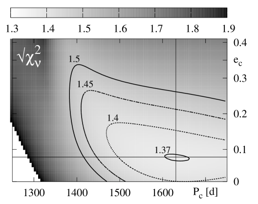
Figure 1: The minimum values of $\sqrt{\chi^{2}_{\nu}}$ as a function of $(P_{{\mbox{\scriptsize c}}},e_{{\mbox{\scriptsize c}}})$ for the 2-Keplerian, Jacobi model of the RV observations ($N_{p}=10+2$). The global minimum is marked by the intersection of two lines, corresponding to $P_{{\mbox{\scriptsize c}}}\simeq 1630$ d, $e_{{\mbox{\scriptsize c}}}\simeq 0.079$. See the text for an explanation.

We verified this fit by determining the quasi-global minimum of $\chi^{2}$ as a function of $(P_{{\mbox{\scriptsize c}}},e_{{\mbox{\scriptsize c}}})$. We searched for the best fit solutions with these two parameters fixed. Because $P_{{\mbox{\scriptsize b}}}$ is determined very well, its value, as well as $e_{{\mbox{\scriptsize b}}}$, approximated by the best GA solution for the 2-Keplerian model, was selected for the starting point in the LM method. Next, varying the initial phases (the arguments of periastron and the mean anomalies) of the two companions, with the step $\simeq 30^{\circ}$, we calculated the best fit solution with the LM algorithm. The results of this experiment are given in Fig. 1. This scan reveals that the best fit solution is localized in a flat minimum. Its parameters agree very well with the GA solution. This test confirmed that the GA fit is really global. Finally, we refined this fit by the LM algorithm, driven by the full model of the dynamics, incorporating the mutual gravitational interaction between the planets. The best GA fit was used as a starting point to the gradient search. The result is shown in Table 1, and named the LM1 fit. The synthetic RV curve is shown in Fig. 2.

To estimate the errors of this solution we used, at the first attempt, a method relying on a determination of the $\chi^{2}$ confidence intervals Press et al. (1992). We were warned by the referees, that this method has drawbacks and the most relevant is that using it we do not account for the stellar “jitter”. Even for a chromospherically inactive HD 12661 star, the uncertainty, $\sigma_{{\mbox{\scriptsize jitter}}}$, contributed by the jitter to the RV measurements, can be relatively high. The referee, Gregory Laughlin, suggested to us using the estimate $\sigma_{{\mbox{\scriptsize jitter}}}\simeq 5$ ms^-1, based on the data by Saar et al. (1998). Actually, the observations have to be weighted by $\sigma=\sqrt{\sigma_{{\mbox{\scriptsize obs}}}^{2}+\sigma_{{\mbox{\scriptsize jitter}}}^{2}}$, where $\sigma_{{\mbox{\scriptsize obs}}}$ are “pure” instrumental errors. Such joint uncertainty, accounted for calculating $\sqrt{\chi^{2}_{\nu}}$, leads to a value $\simeq 1$, thus giving a statistical indication of an adequate model of the RV data. To estimate the parameters errors we synthesized about $250$ sets of “observations”. To every original RV measurement we added a Gaussian noise with the mean dispersion $\sigma_{{\mbox{\scriptsize K}}}=3.4$ ms^-1, $\sigma_{{\mbox{\scriptsize L}}}=7.6$ ms^-1 for observations gathered by Keck and Lick spectrometers, respectively, and the Gaussian noise of the stellar jitter, with the dispersion $\sigma_{{\mbox{\scriptsize jitter}}}=5$ ms^-1. Next, the Newtonian model of dynamics was fitted to every such synthetic data set with the LM algorithm which started from the LM1 solution. The mean values of the fit parameters are given in Table 1, and called the LM2 fit. Finally, the dispersions of these orbital parameters are adopted as the mean uncertainties of both the LM1 and LM2 fits. In fact, both solutions are the same, with respect to the error bounds.

3 Stability analysis

To investigate the dynamical stability of the LM1 and LM2 fits we used the fast indicator called MEGNO. This technique was advocated by us in a series of recent papers, see, e.g,  Goździewski et al. (2001); Goździewski (2003). The MEGNO indicator is closely related to the maximal Lyapunov exponent, but it permits to determine rapidly whether an initial condition leads to a regular, quasi-periodic or a chaotic, irregular solution. It is a very efficient tool that helps to detect orbital resonances, their structure, and unstable regions in the phase space. Looking at a neighborhood of the analyzed initial conditions is a profitable way of resolving the question whether the system dynamics are robust to the fit errors.

The MEGNO tests reveal that both the LM1 and LM2 fits are related to quasi-periodic motions of the HD12661 system. The MEGNO signature for the LM1 fit is shown in Fig. 4c and a perfect convergence of the temporal value of MEGNO to 2 indicates a quasi-periodic evolution of the planetary system. The MEGNO scan in the neighborhood of this fit, in the ($a_{{\mbox{\scriptsize c}}},e_{{\mbox{\scriptsize c}}})$-plane, is shown in the left panel of Fig. 3. Actually, both fits are located in a relatively extended stable zone, in a proximity of the the 6:1 MMR. The 6:1 MMR is separated about $0.2$ au from the 11:2 MMR, which has been considered, up to now, as the closest MMR neighboring the system in the phase space. The evolution of orbital elements in the LM1 fit is shown in Fig. 4a,b.

The stable zone of the 6:1 MMR is relatively very narrow in the range of small $e_{{\mbox{\scriptsize c}}}$. To illustrate its effect on the motion of the HD 12661 system we changed $a_{{\mbox{\scriptsize c}}}$ in the LM2 fit, from the nominal value $\simeq 2.78$ au to $2.745$ au, still keeping it in the error bound. The MEGNO scan, in the ($a_{{\mbox{\scriptsize c}}},e_{{\mbox{\scriptsize c}}})$-plane, for such modified initial condition is shown in the right panel of Fig. 3, and the Jacobi elements are shown in Fig. 4d,e,f. Note that in both cases the SAR with the apsidal lines antialigned in the exact resonance is present, so the system still remains in the large libration island found by Lee & Peale (2003).

The scan in the $(i,\Delta\Omega)$-plane, where $\Delta\Omega=\Omega_{{\mbox{\scriptsize c}}}-\Omega_{{\mbox{\scriptsize b}}}$, is shown in Fig. 5, and it makes is possible to estimate the bounds on masses in the systems with the same $i$, in terms of regular and chaotic motions. For coplanar systems, the stable zone extends up to $i\simeq 25^{\circ}$, but also two islands about $i\simeq 10^{\circ},18^{\circ}$ exist. Whether the system can survive during evolutionary time scales, in the chaotic regions, can be verified, in general, only by long-term integrations.

Conclusions

The study of the RV observations of the HD 12661 star revealed fits which lead to significantly different dynamics when compared to the original solution published by Fischer et al. (2003). Combined genetic and gradient methods of optimization helped us to find a global minimum of $\chi^{2}$ for the RV model that incorporates the mutual interactions between planets. A dynamical analysis shows that the new fits are related to a system close to the 6:1 MMR, and locked into a deep secular resonance with apsidal lines antialigned. The fits preclude the proximity of the 11:2 MMR, which has been suggested by the previously determined initial conditions. In the phase space, the system lies in a relatively extended zone of stable, quasi-periodic motions. The closeness of the HD 12661 system to the low-order 6:1 MMR adds a new inquiring case to the 3:1 MMR in the 55 Cnc system, the 7:3 MMR in the 47 UMa system, and the 5:2 MMR of Jupiter and Saturn. It is difficult to claim that the HD 12661 system is locked exactly in the 6:1 MMR, but our results suggest that very likely it is close to this resonance. Hopefully, the observational window of the HD 12661 will cover soon two orbital periods of the outer companion, and the updated set of measurements will help to refine the fits again.

The analysis of the RV data benefits from a global approach, similarly to the stability studies. For planetary systems with large, and not very distant planets, the effects of mutual interactions and a proper dynamical interpretation of the orbital fits are vital for understanding the dynamics and for resolving all the information hidden in the observations. Their analysis requires much care, because omitting even subtle factors can lead to quite a different interpretation of the same data set.

Table 1: Osculating, astrocentric Keplerian elements of the HD 12661 planetary system for the epoch of the first observation (JD=2450831.608). Mass of the host star is 1.07 $M_{\sun}$.

Fit	LM1 ($N_{p}$=10+2)		Mean (LM2) ($N_{p}$=10+2)
Parameter	Planet b	Planet c	Planet b	Planet c
$\mbox{m}_{{\mbox{\scriptsize pl}}}\sin i$ [MJ]	2.33 (0.04)	1.69 (0.11)	2.32 (0.04)	1.63 (0.11)
$a$ [au]	0.822 (0.001)	2.804 (0.11)	0.823 (0.001)	2.781 (0.11)
$e$	0.349 (0.016)	0.084 (0.054)	0.343 (0.016)	0.128 (0.054)
$\omega$ [deg]	115.2 (3.9)	292.8 (34.1)	113.8 (3.9)	303.1 (34.1)
$M$ [deg]	129.4 (4.7)	354.3 (42.9)	132.1 (4.7)	342.5 (42.9)
$V_{0}$ (Lick) [ms-1]	-7.3 (1.9)		-6.3 (1.9)
$V_{1}$ (Keck) [ms-1]	-12.7 (1.9)		-12.2 (1.9)
$\sqrt{\chi^{2}_{\nu}}$	1.37		0.93
RMS [ms-1]	7.88		7.44

Figure 2: The synthetic radial velocity curve defined by the LM1 fit (see Table 1). Time is given in JD. Filled circles mark the observations published by Fischer et al. (2003).

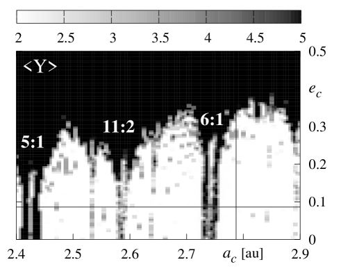
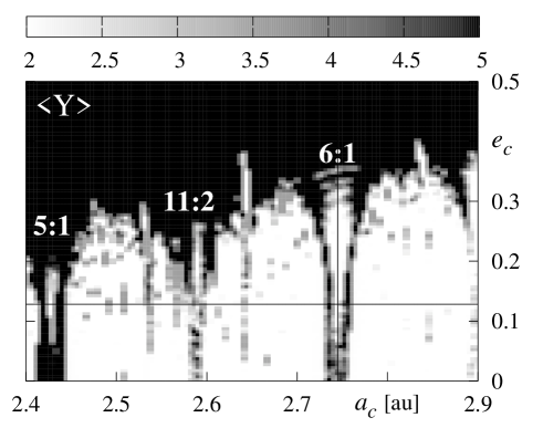
Figure 3: The MEGNO maps in the $(P_{{\mbox{\scriptsize c}}},e_{{\mbox{\scriptsize c}}})$-plane for the initial elements found in this paper. The left panel is for the LM1 fit, the right panel is for the modified LM2 fit (as explained in the text). Zones centered about $\simeq 2$ correspond to regular, quasi-periodic motions of the HD 12661 system. The intersection of two lines marks the fitted parameters, the MMRs relevant to our discussion are labeled. The resolution of the scan is $120\times 100$ data points.

Figure 4: The evolution of Keplerian orbital elements related to Jacobi coordinates for the initial conditions found in this paper. The left column is for the LM1 fit, the right column is for the modified LM2 fit. Note the presence of the secular apsidal resonance—its critical argument $\varpi_{{\mbox{\scriptsize b}}}-\varpi_{{\mbox{\scriptsize c}}}$ librates about $180^{\circ}$ (panels b,e). The modified LM2 fit leads to the 6:1 MMR (panel f), while for the LM1 fit the same critical argument circulates. Note the stabilizing effect of the 6:1 MMR on the eccentricities of the planets (panels a,d). Panel c is for MEGNO signature of the LM1 fit and it indicates a quasi-periodic, stable motion of the planetary system. Time is given in $10^{5}$ yr.

Figure 5: Stability regions in the plane of the system inclination $i$ vs the relative inclination of orbits (expressed through the difference of the longitudes of nodes, $\Delta\Omega=\Omega_{{\mbox{\scriptsize c}}}-\Omega_{{\mbox{\scriptsize b}}}$), derived for the LM2 fit. The resolution of the scan is $85\times 90$ data points.

References

- Butler et al. (1999) Butler, R. P., Marcy, G. W., Fischer, D. A., Brown, T. M., Contos, A. R., Korzennik, S. G., Nisenson, P., & Noyes, R. W. 1999, ApJ, 526, 916
- Charbonneau (1995) Charbonneau, P. 1995, ApJS, 101, 309
- Fischer et al. (2003) Fischer, D. A., Marcy, G. W., Butler, R. P., Vogt, S. S., Henry, G. W., Pourbaix, D., Walp, B., Misch, A. A., & Wright, J. 2003, ApJ, preprint doi:10.1086/367889
- Goździewski (2003) Goździewski, K. 2003, A&A, 398, 1151
- Goździewski et al. (2001) Goździewski, K., Bois, E., Maciejewski, A., & Kiseleva-Eggleton, L. 2001, A&A, 378, 569
- Goździewski et al. (2003) Goździewski, K., Konacki, M., & Maciejewski, A. 2003, ApJ, in preparation
- Laughlin & Chambers (2001) Laughlin, G. & Chambers, J. E. 2001, ApJ, 551, L109
- Lee & Peale (2003) Lee, M. H. & Peale, S. J. 2003, ApJ, submitted
- Marcy et al. (2002) Marcy, G. W., Butler, R. P., Fischer, D. A., Laughlin, G., Vogt, S. S., Henry, G. W., & Pourbaix, D. 2002, ApJ, 581, 1375
- Press et al. (1992) Press, W. H., Teukolsky, S. A., Vetterling, W. T., & Flannery, B. P. 1992, Numerical Recipes in C. The Art of Scientific Computing (Cambridge Univ. Press)
- Rivera & Lissauer (2001) Rivera, E. J. & Lissauer, J. J. 2001, ApJ, 402, 558
- Saar et al. (1998) Saar, S. H., Butler, R. P., & Marcy, G. W. 1998, ApJ, 498, L153+
- Stepinski et al. (2000) Stepinski, T. F., Malhotra, R., & Black, D. C. 2000, ApJ, 545, 1044