Anisotropies in the redshift-space correlations of galaxy groups and clusters I: Simulated catalogues

Abstract

We analyse the correlation function of mock galaxy clusters in redshift space. We constructed several mock catalogues designed to mimic the selection biases inherent in a variety of observational surveys. We explore different effects that contribute to the distortion of the clustering pattern; the pairwise velocity distribution of galaxy systems, coherent bulk motions, redshift errors and systematics in cluster identification. Our tests show that the redshift-space clustering pattern of galaxy systems is highly influenced by effects associated with the identification procedure from two dimensional surveys. These systems show a spuriously large correlation amplitude, an effect that is present and even stronger in a subsample whose angular positions coincide with 3-dimensional identified clusters. The effect of a small number of redshift measurements is also that of increasing the correlation amplitude. In a similar fashion, the bias parameter inferred from cluster samples is subject to these observational problems which induce variations of up to a factor of two in such determinations. Also, we find that the estimated mean pairwise velocity dispersion can be up to an order of magnitude larger than the actual value. Errors in the estimated cluster redshift, originating from the use of too few redshift measurements per cluster, have a smaller impact on the measured correlation function. We show that an angular incompleteness in redshift surveys, such as that present in the 2dFGRS 100k public release, has no significant effect in the results. We suggest that the nature of projection effects arise mainly from structures along the line of sight in the filamentary large-scale clustering pattern. Thus, spectroscopic surveys are the only means of providing unbiased cluster samples.

1 Introduction

Rich clusters of galaxies form at the highest peaks of the mass distribution through physical processes which are simpler than those involved in galaxy formation. As a consequence, models show that the correlation function and power spectrum of clusters of galaxies have the same shape as that of the mass, with an amplitude depending on a small number of parameters (see for example Colberg et al. 2000, Sheth, Mo & Tormen 2001, Padilla & Baugh, 2002). In fact, the space density of clusters of galaxies is usually the only parameter needed to obtain a direct estimate of the underlying mass distribution (Padilla & Baugh, 2002). This shows the clear advantage of studying clusters of galaxies, which has made them popular tracers of the large scale structure of the Universe in the literature.

Cluster distances are derived from member galaxy redshifts, which are affected by galaxy peculiar velocities. Even if all the member galaxy redshifts are used in the determination of the cluster distance, this will be still affected by the cluster peculiar motion, and will not be a true distance measurement. The distribution function of cluster peculiar motions depends upon the value of the mass density parameter $\Omega$, for models with similar mass fluctuation amplitudes (Croft & Efstathiou 1994a; Bahcall, Cen & Gramann 1994). These motions, either for galaxies or clusters of galaxies, produce an apparent distortion of the clustering pattern as measured by the two-point correlation function in redshift space, $\xi(\sigma,\pi)$, where $\sigma$ and $\pi$ are the separations perpendicular and parallel to the line of sight, respectively. At small separations, non-linear, nearly virialized regions produce elongations along the line of sight which allow measurements of the one-dimensional pairwise rms velocity dispersion, $<w_{12}^{2}>^{1/2}$ (Davis & Peebles 1983). Larger scales are dominated by the infall onto overdense regions in the form of bulk motions which result in a compression of the $\xi$ contours along the direction of the line of sight.

Evidence of strong anisotropies in the correlation function of Abell clusters has been given by several authors (see for instance Postman, Huchra & Geller 1992 and references therein). Systematic effects in the Abell catalogue originate in the superposition of clusters along the line of sight and generate a bias in the observed correlation function of the catalogue (Sutherland 1988; Sutherland & Efstathiou 1991; see also Lucey 1983). Using mock catalogues from numerical simulations, van Haarlem et al. (1997) showed that a large fraction of Abell clusters of richness class $R\geq 1$ would not be physically bound systems and would suffer from contamination by galaxies and groups along the line of sight. Therefore it is likely that the observed large anisotropies could be mainly produced by systematics in cluster detection algorithms from angular galaxy catalogues.

The construction of objectively defined cluster catalogues drawn from machine-scanned survey plates with better calibrated photometry brought a new generation of cluster catalogues which are believed to be less affected by identification biases (APM: Dalton et al. 1992, 1994, 1997; Cosmos: Lumsden et al. 1992). The typical radius used to define clusters in the machine based catalogues is significantly smaller than that used by Abell, reducing the enhancement of cluster richness by projection effects. The clustering signal found in these more recent cluster redshift surveys does not display large enhancements along the line of sight; furthermore, the trend of increasing correlation amplitude with decreasing space density of clusters is weaker than that found for Abell clusters (Croft et al. 1997) and is similar to the trend expected in current models of structure formation. A similarly weak dependence of correlation length on cluster space density is found in X-ray selected cluster catalogues, such as the X-ray Bright Abell Cluster Sample (XBACS) and the REFLEX sample (Collins et al. 2000), which are less susceptible to line of sight projection effects than the optically selected Abell catalogue (Abadi, Lambas & Muriel 1998; Borgani et al. 1999). However, Miller et al. (1999) argue that the early redshift surveys of Abell clusters contain large fractions of low richness clusters (Abell richness class $R=0$), which were not intended to form complete samples suitable for statistical analyses. Miller et al. (1999) present the clustering analysis of a new redshift survey of Abell clusters with richness $R\geq 1$, and with the majority of cluster positions determined using several galaxy redshifts. The clustering signal along the line of sight is greatly reduced in the new redshift surveys compared with the Bahcall & Soneira (1983) results, and is comparable to the amount of distortion of the clustering pattern found for APM clusters (see Fig 5 of Miller et al. 1999). The anisotropy is further reduced after the orientation of two superclusters that are elongated along the line of sight is changed. Peacock & West (1992) also found that restricting the attention to higher richness Abell clusters removed the strong radial anisotropy seen in the clustering measured in the earlier surveys.

Another possible source of systematics could rely on the fact that several cluster distances are determined by a single galaxy redshift, usually the brightest cluster member. Therefore it is important to explore the effects of cluster distance errors on the analysis of correlation function of rich clusters.

The gravitational amplification of small primordial fluctuations has been analysed through numerical simulations to explore the spatial distribution of clusters (e.g. White et al. 1987; Bahcall & Cen 1992; Croft & Efstathiou 1994b; Watanabe, Matsubara & Suto 1994; Eke et al. 1996). These early studies do not reach a consensus on the predicted clustering of clusters in cold dark matter cosmologies. Part of the reason for this discrepancy is due to differences in the way in which clusters are identified in the simulations (Eke et al. 1996). More recent studies have made use of much larger volumes than in these earlier studies, with sufficient resolution to allow the reliable extraction of massive dark matter haloes that can be identified as rich clusters (Governato et al. 1999; Colberg et al. 2000, Jenkins et al. 2001).

In this paper, we analyse the redshift space clustering of massive dark matter haloes in mock catalogues extracted from the $\tau$CDM Hubble Volume simulation. In particular, we use the mock catalogues made available by the Virgo Consortium, which contain galaxy angular positions and distances, with a redshift distribution set by a selection function. In this work we will make use of these mock catalogues to analyse in detail the effects of projection biases on catalogues of clusters identified in two dimensions. We also predict the results of the new generations of cluster catalogues with a high degree of spectroscopic completeness such as the 2dF Galaxy Redshift Survey (Norberg et al. 2002).

The outline of this paper is as follows: section 2 describes the equations which allow us to obtain a statistical description of the redshift-space correlation function as a function of coordinates parallel and perpendicular to the line of sight, through the pairwise velocity dispersions, redshift-space correlation length and bias parameters; section 3 presents the correlation function measurement technique. Section 4 presents the different mock cluster samples constructed using several cluster identification algorithms, and studies the results arising from using different number of redshifts to derive cluster distances and also different values of the search radius in cluster identification. In this section, we also study the dependence of the relative pairwise velocities, redshift-space correlation length and bias factors as a function of the number of redshifts used in the determination of the cluster distances. In section 5 we discuss our results and present the main conclusions drawn from this work.

2 Redshift-space correlation function anisotropy

The redshift-space correlation function can be calculated as a function of the pair separation parallel and perpendicular to the line of sight. This approach has led to the quantification of characteristics of the redshift-space distribution of galaxy and clusters of galaxies, such as the ”fingers of God”, which are elongated structures seen in redshift surveys, originated from the random motions of galaxies inside clusters.

The strength of the “fingers of god” effect depends on the pairwise velocities of galaxies, which so far has been measured using two different methods. The first method corresponds to that adopted by Loveday et al. (1996) and Ratcliffe et al. (1998), which compares a theoretical expression for the correlation function with the measured values, $\xi^{m}(\sigma,\pi)$ (the index $m$ indicates measured quantities), in a grid of values of distances parallel and perpendicular to the line of sight. The other approach presented by Padilla et al. (2001), compared the isopleths (curves of equal correlation function amplitude) in the measured and predicted correlation functions. The $\xi(\sigma,\pi)$ contour levels are approximated by the functions $r^{m}(\theta)$ and $r^{p}(\theta)$ for the measured and predicted correlations respectively. Here $\theta$ is the polar angle measured from the direction perpendicular to the line of sight (Padilla et al. 2001), such that $\xi^{x}(\sigma_{r},\pi_{r})-\xi^{fix}=0$, where $\sigma_{r}=r^{x}_{\xi^{fix}}(\theta)\cos(\theta)$, $\pi_{r}=r^{x}_{\xi^{fix}}(\theta)\sin(\theta)$, and the index $x$ indicates either measured ($m$) or predicted quantities ($p$).

In either method, the measured correlation function $\xi^{m}(\sigma,\pi)$ is compared with the convolution of the real-space correlation function, $\xi(r)$ with the pairwise velocity distribution function, $f(w)$, following Bean et al. (1983). We calculate

$$1+\xi^{p}(\sigma,\pi)=\int_{-\infty}^{\infty}[1+\xi(r)]f[w^{\prime}-w^{s}(r,r^{\prime})]{\rm d}w^{\prime},$$ (1)

where $r^{2}=r^{\prime 2}+\sigma^{2}$, and $H_{0}$ is the Hubble constant, $r^{\prime}=\pi-w^{\prime}/H_{0}$ (the prime denotes the line-of-sight component of a vector quantity) and

$$w^{s}(r,r^{\prime})\simeq-H_{0}\beta\xi(r)(1+\xi(r))^{-1}r^{\prime},$$ (2)

is the mean streaming velocity of galaxies at separation $r$.

Following usual procedures we calculate the best-fit rms peculiar velocity, $<w^{2}>^{1/2}$, for an exponential distribution,

$$f(w)=\frac{1}{\sqrt{2}<w^{2}>^{1/2}}\exp\left(-\sqrt{2}\frac{|w|}{<w^{2}>^{1/2}}\right).$$ (3)

We adopted this pairwise velocity distribution as it has shown to be the most accurate fit to the results from numerical simulations (Ratcliffe et al. 1998).

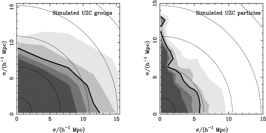
Figure 1: The 2-point correlation function of simulation groups (left hand side panel) and simulation particles (right panel) in the coordinates $\sigma$ and $\pi$ (mock group and galaxy samples from Padilla et al., 2001). From light to dark, the transitions between different shadings correspond to fixed level values of $\xi=0.6,0.8,1.0,1.2,$ and $1.4$, which are later used to infer the relative pairwise velocities, $w_{12}$. The thick line corresponds to the $\xi=1$ level, and the thin lines show the expected contours in the absence of peculiar velocities.

Two estimates of the real-space correlation function are usually adopted in equation 1: the inversion of the projected correlation function (Baugh 1996, Ratcliffe et al. 1998), or a simple power-law fit obtained from the angular correlation function (Padilla et al. 2001). In this work we use the theoretical correlation function of the simulated mass distribution and adopt a linear bias parameter $b$ that relates clusters and mass by Fourier transforming the model power spectrum

$$\xi^{CDM}(r)=\frac{1}{2\pi^{2}}b^{2}\int_{0}^{\infty}P(k)\frac{\sin(kr)}{kr}k^{2}{\rm d}k,$$ (4)

We use this to evaluate the theoretical prediction for $\xi^{p}(\sigma,\pi)$ using equation (1). We search for the optimum values of the scale independent bias parameter $b$ and $<w^{2}>^{1/2}$ by minimising the quantity $\chi^{2}$,

$$\chi^{2}=\sum_{i}[r^{m}_{l}(\theta_{i})-r^{p}_{l}(\theta_{i})]^{2},$$ (5)

where we have chosen to compare a set of discrete levels, $l=0.6,0.8,1.0,1.2$ and $1.4$, of the redshift-space correlation function $\xi(\sigma,\pi)$ amplitude instead of comparing values of the correlation function on a grid of $\sigma$ and $\pi$ distances. Our choice is based on the fact that more reliable and stable results are obtained using this technique (Padilla et al. 2001).

3 Measuring $\xi(\sigma,\pi)$

We have computed $\xi^{m}(\sigma,\pi)$ as a function of the separation perpendicular ($\sigma$) and parallel ($\pi$) to the line of sight. To compute $\xi^{m}(\sigma,\pi)$, we generate a random catalogue with the same angular limits and radial selection function as the sample of objects. We cross correlate data-data and random-random pairs ($N_{dd}$ and $N_{rr}$ respectively) binning them as a function of separation in the two variables $\sigma$ and $\pi$. Our estimate of $\xi^{o}(\sigma,\pi)$ is (Davis & Peebles 1983):

$$\xi^{m}(\sigma,\pi)=\frac{N_{dd}n_{R}^{2}}{N_{rr}n_{D}^{2}}-1$$ (6)

where $n_{D}$ and $n_{R}$ are the number of data and random points respectively.

This estimator is affected by uncertainties in the mean density, in particular on large scales where $\xi(r)$ is small (eg. Hamilton 1993). However, since our analysis is confined to small separations where the correlation function has a large amplitude, our results are insensitive to the choice of estimator.

Figure 1 shows the contours of equal amplitude of the 2-point correlation function of groups identified in a numerical simulation (left panel) and simulation particles (right panel) in the coordinates $\sigma$ and $\pi$ (mock galaxy and group samples from Padilla et al. 2001). The compression of the iso-correlation curves for groups in the $\pi$ direction can be appreciated, indicating a lack of high pairwise velocities in this sample. From the comparison with results derived from clusters identified in two-dimensional surveys (see for instance Bahcall, Soneira & Burgett, 1986) the existence of either large pairwise velocities or large projection biases is clear, as also discussed by Sutherland (1988).

This elongation could originate in the systematic presence of groups along the line of sight, in the fields of clusters identified from angular data. From the theoretical point of view, such strong elongations along the line of sight are not expected in a hierarchical scenario of structure formation. This is confirmed by the compression observed in left hand side panel of figure 1 and provides a clear evidence for the infall of groups onto larger structures (see also Peacock et al. 2001, for galaxies). As the contours are well defined for all the correlation function levels shown in this figure ($\xi=0.6$, $0.8$, $1.0$, $1.2$ and $1.6$), the analysis developed in the next sections will be based on the results at these contours. In the right hand side panel, the large distortion seen in the iso-correlation curves in the $\pi$ direction is due to the larger peculiar velocities of the simulation particles and their smaller correlation amplitude, associated with the non-linear evolution of the density field on small scales.

4 Results from mock catalogues extracted from N-body simulations

In this section, we analyse the statistical properties of cluster samples drawn from mock catalogues. These mock catalogues have been obtained from one of the mock galaxy catalogues extracted from the $\tau$CDM Hubble Volume simulation by the Durham Extragalactic Group (Evrard et al., 2002) following a procedure similar to that used in Cole et al. (1998). This simulation follows the evolution of cold dark matter (CDM) density fluctuations in a $\tau$CDM cosmology, with parameters $\Omega_{0}=1.0$, a cosmological constant $\Lambda_{0}c^{2}/(3H_{0}^{2})=0$, and a power spectrum described by a shape parameter of $\Gamma=0.21$ and $\sigma_{8}=0.6$. The huge volume of the simulation ($8h^{-3}{\rm Gpc}^{3}$) and the large number of particles employed ($10^{9}$) allow cluster statistics to be studied with unprecedented accuracy (Colberg et al. 2000; Jenkins et al. 2001).

The particular mock catalogue we chose to apply the different identification methods to, is that of the APM survey, with a selection function consistent with a limiting magnitude $b_{J}=20.0$.

This particular mock catalogue has the advantage that the derived galaxy apparent magnitudes have $k+e$ corrections which reproduce the results of the 2dFGRS (see Norberg et al. 2002, for details). Also we notice that the observer is not chosen at random but instead constrained to lie in a region with similar properties to those of the Local Group.

4.1 Mock Groups identification

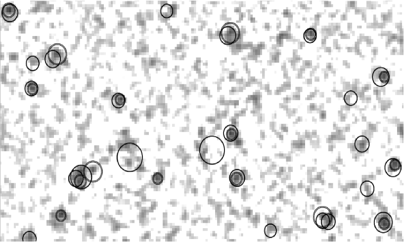
Figure 2: Galaxy density and clusters in the mock catalogues. The density of galaxies in the pixelmap is proportional to the darkness of the pixels in this figure. The double-line circles show clusters from mock sample 3, whereas thick-line circles indicate the positions of clusters in mock sample 2. This figure shows a sub-set of the pixelised mock galaxy catalogue and is shown in an equal area projection centred at $\alpha=1^{h}$ and $\delta=-45^{o}$, with radius $r_{eqa}=160^{o}$. The number of pixels per side is $n_{pix}=2900$, and was set in order to obtain a mean number of galaxies $n=1$ per pixel. The pixelmap sub-set size is $170{\rm x}90$ pixels.

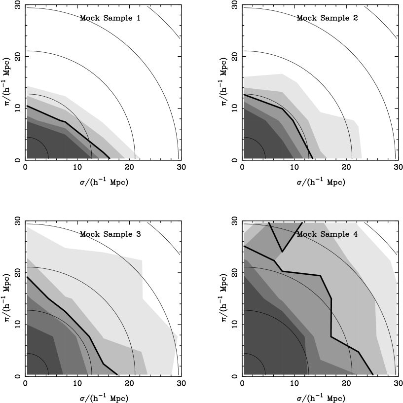
Figure 3: $\xi(\sigma,\pi)$ from simulated catalogues of clusters of galaxies with distances measured using $10$ member galaxies, obtained using different algorithms. Upper left panel shows the results from sample 1, upper right panel from sample 2, lower left panel shows the contours obtained from sample 3, and the lower right panel, those from sample 4. Shadings and line conventions are as in figure 1.

We use three main algorithms to search for groups in the numerical simulations, and construct four samples of clusters from them:

• Sample 1, is constructed using a friends-of-friends algorithm applied to the 3-dimensional distribution of particles in the simulation cube. We used a linking length $b=0.2$, expressed in terms of the mean interparticle separation, adequate for the $\tau$CDM cosmology (Helly et al., 2003). This sample is almost completely free of spurious clusters since we have chosen to study only those groups with at least $60$ member particles. The fraction of unbound associations found using FOF drops quickly as the number of member particles rises over $10$.

  Given the lack of a significant number of spurious clusters, the measurements of anisotropies in the correlation function should clearly show the expected infall pattern. As we do not have computational access to the full Hubble Volume simulations, we applied the FOF identification algorithm to a numerical simulation with box size $600$h^-1Mpc with exactly the same cosmological parameters as the $\tau$CDM simulation. This ensures that this particular sample of clusters is statistically comparable to those obtained from the mock galaxy catalogue produced by the Durham group.

• Sample 2 comprises the results from the identification of groups in a mock catalogue that includes a selection function, and where the position of particles is determined from redshifts, that is including particle peculiar velocities. We use a friends-of-friends algorithm with different linking lengths in the directions parallel and perpendicular to the line of sight. This procedure emulates the identification process used in the construction of the group sample obtained from the Updated Zwicky Catalogue, which is based on an algorithm described by Huchra & Geller (1982). In this case we use different linking lengths in the directions perpendicular and parallel to the line of sight, which vary linearly with distance, $d_{0}=V/V_{fid}0.229$h^-1Mpc and $v_{0}=V/V_{fid}350$km/s, where $V$ is the distance, and $V_{fid}=7000$km/s. These values correspond to a density contrast $\delta\rho/\rho\simeq 80$.

• Sample 3 is obtained using the algorithm presented by Lumsden et al.(1992), which is used in identifying clusters from the COSMOS catalogue. Following the prescription described by Lumsden et al. (1992), we use an angular search radius $r_{c}=1.0$h^-1Mpc, and apply this procedure to the same mock catalogues as the second algorithm. We tested this identification algorithm by applying it to the COSMOS galaxies, and comparing the outcome of the identification algorithm to the positions of the EDCC clusters (Lumsden et al. 1992). We found out that $\sim 75\%$ of the EDCC clusters were re-obtained by our identification procedure. We also applied this to a numerical simulation, and found that only $\sim 70\%$ of the clusters identified in the simulation cube with a FOF algorithm were found by our angular identifier. More importantly, only $\sim 60\%$ of the clusters identified are real clusters. These numbers illustrate the degree of projection effects sample 3 is subject to, and its study will serve as a test of how these effects translate into the cluster correlation function in redshift-space.

• Sample 4: We extract from sample 3 the subset of clusters whose angular positions are coincident (within the cluster identification radius) to those in sample 2. This sample is derived from a 2 dimensional catalogue and is confirmed to have a redshift space identification at the same angular position. Cluster distances are determined by using the galaxy members identified from the angular position data. This sample should be less affected by projection effects than that obtained from the angular data alone. However, cluster distances may include particles that are not physically related to any particular cluster at all. We find that only $\sim 50\%$ of the clusters from sample 3 are present in this sample indicating that this procedure provides a significant restriction. We also notice that this fraction is slightly different than that resulting from comparing the sample 3 clusters with those obtained from using the FOF algorithm on a full simulation box.

All the samples defined in this section include groups with a minimum mass threshold. This threshold is set so as to make the space density of all the samples as close to that of sample 1 as possible.

In figure 2. we show the different results from the identification of clusters of galaxies in the mock catalogue using angular and 3-D galaxy positions. This figure shows the density of galaxies in the mock catalogue in pixels, and clusters of galaxies in circles. The gray scale of the pixels indicate number of galaxies; the darker the pixel the higher is the number of galaxies in it. As can be seen, the circles enclose regions of high density of galaxies. The different line styles with which the circles are drawn correspond to the different algorithms used in the identification of clusters. The double-line circles correspond to clusters from sample 3, that is, clusters identified using angular data. In this case, the radius of the circle corresponds to the radius out to which the counting of galaxies was done when measuring the cluster richness. The thick line circles show clusters from sample 2, identified from 3-dimensional positions affected by the peculiar velocities of the clusters. In this case, the radius of the circle is proportional to the richness of the clusters. By inspection to this figure, we can appreciate the large fraction of clusters from sample 3 whose angular positions are not coincident with any 3-dimensional cluster within one angular search radius.

The aim of constructing the mock cluster samples presented here is to understand and reproduce the results obtained from observational cluster samples. In particular, we intend to establish the reason for the large elongations along the line of sight present in the measured correlation functions. The different behaviours of the correlation functions found for the four mock samples are shown in figure 3, where we used clusters of galaxies with distances measured using $10$ member galaxies. The results from samples 1 and 2 show the expected infall pattern. This simply indicates that the FOF algorithm still works well when applied to a catalogue which incorporates a selection function and includes the effects of galaxy peculiar velocities. The infall is not so evident when inspecting the remaining panels, which simply show the different degrees of projection effects the different samples are subject to. It can be seen that samples 3 and 4 show somewhat large elongations along the line of sight. Taking into account that all panels show the results for the same value of $n_{z}=10$, this is a clear signature of projection effects. The fact that sample 4 shows elongated contours along the line of sight is indicative of substantial projection contamination. Given that we have constructed this sample by requiring an angular coincidence between 2-dim and 3-dim identified clusters, such anisotropies reflect the fact that there is a strong contribution by other structures along the line of sight in producing the observed distortion pattern.

In the following section we provide detailed descriptions of the characteristics of each sample, analysing the differences in elongations arising from using different $n_{z}$.

4.2 Effects of observed number of redshifts

In order to make a thorough comparison between the mock cluster samples and the observational correlation functions, we study in detail the effects of using different $n_{z}$ in each of our mock samples.

We first show the results from sample 1 which comprises clusters of galaxies identified from the 3-dimensional distribution of particles in the full numerical simulation. Figure 4 shows the correlation function contours when the distances to the clusters in this sample have been calculated using $1$ (left) and $20$ (right panel) member redshifts. As can be seen, the differences between the panels are quite small. The left panel only shows slight evidence of an elongation along the line of sight. This is an effect produced by the errors in the distance to these clusters arising from the use of only one redshift to determine their distances. By comparison between the left upper panel in figure 3 and the right panel in figure 4 (that is, Sample 1 with $n_{z}=10$ and $20$), it can be seen that the use of a small $n_{z}=10$ is sufficient to erase spurious elongations along the line of sight, and that considering more redshifts per cluster makes no significant difference. This result once more reflects the reliability of the FOF algorithm in finding clusters of galaxies in numerical simulations.

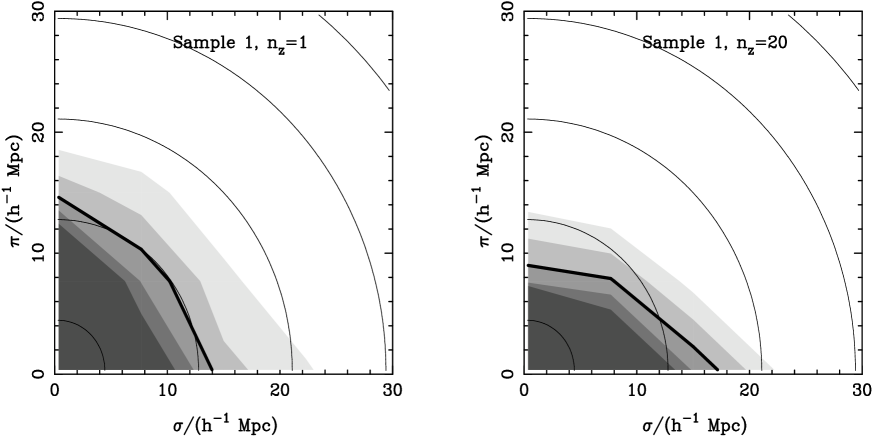
Figure 4: The correlation function contours for clusters identified using the FOF algorithm from the simulation (mock sample 1). The different panels correspond to different $n_{z}$: $1$ redshift measurement (left) and $20$ (right) member redshifts. Shadings and line conventions are as in figure 1.

We now investigate the effects of changing $n_{z}$ in sample 2, which consists of clusters identified from a mock galaxy catalogue which incorporates a selection function. We show in figure 5 the correlation function contours for samples with distances obtained using $1$ and $20$ redshifts in the left and right hand side panels respectively. As can be seen in this figure, the effects of using a small $n_{z}$ are not critical. In the case of using $1$ galaxy, the infall pattern can still be seen, specially in the correlation contours corresponding to $\xi(\sigma,\pi)<1$. The inclusion of further redshifts only makes a small change, although it can be seen that in this case, this signature is also visible for levels of higher correlation function. When comparing with figure 4 one can notice a neat infall pattern in the clusters from sample 1 for high levels of correlation even when $n_{z}=20$ (a very clear signature for $\xi=1$ contour levels, and mildly visible for $\xi=1.4$). The case of sample 2 is less ideal, since this infall pattern can only be marginally seen for a correlation function contour level corresponding to $\xi=1$, which simply reflects the higher degree of difficulty in identifying clusters from a galaxy catalogue which incorporates a selection function.

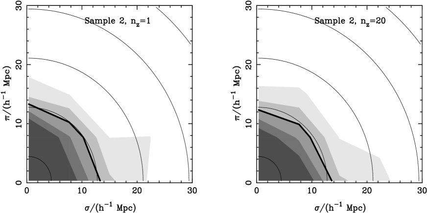
Figure 5: Correlation function contours for the cluster mock sample 2 which comprises clusters identified using a modified version of the FOF algorithm, applicable to a mock redshift survey, which includes peculiar velocities and a selection function. We show the results for cluster distances obtained using $1$ and $20$ redshifts in the left and right panels respectively. Shadings and line conventions are as in figure 1.

It should be noted that sample 2 is representative of cluster or group catalogues identified in galaxy redshift surveys, as is the case with UZC groups. Therefore, the infall of structures which is a signature of the hierarchical clustering obtained in the correlation function contours measured using the UZC groups sample (Padilla et al. 2001), can be assessed by the results of sample 2. In other words, the study arising from sample 2 results in a correlation function which is not badly affected by projection effects, even for small $n_{z}$, which also indicates that the use of a small $n_{z}$ does not induce important elongations along the line of sight.

We next consider a mock cluster catalogue drawn from an angular galaxy catalogue (sample 3). Here the distances to each cluster were obtained using the redshifts of galaxies identified as cluster members using angular data. The correlation function of these catalogues are shown in figure 6, where we show the results when using $1$, $5$, $10$, and $20$ galaxy redshifts in determining cluster distances in the upper left, upper right, lower left and lower right panels respectively.

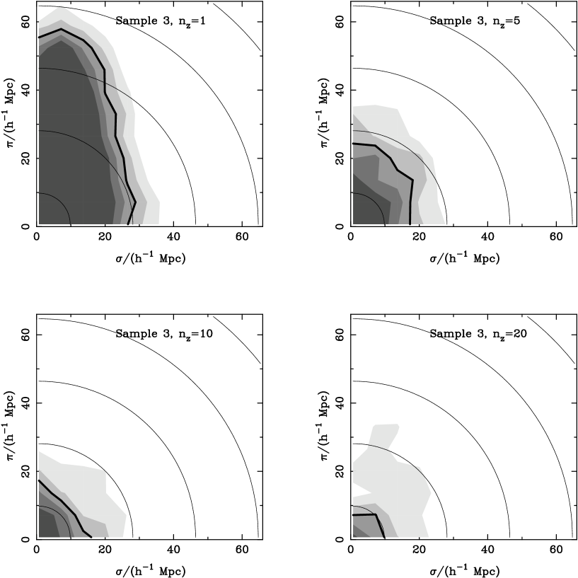
Figure 6: Correlation function isopleths obtained from clusters identified from angular positions drawn from the numerical simulation (mock cluster sample 3), with $1$, $5$, $10$, and $20$ individual redshift measurements in panels upper left, upper right, lower left, and lower right respectively. Shadings and line conventions are as in figure 1.

The results in this figure show significant differences in the elongations for the different samples. In the case where only $1$ galaxy redshift is used to assess the cluster distance, the elongation along the line of sight is severe, and not entirely different to what was found for Abell clusters with distances estimated using less than $10$ galaxy redshifts (see for instance Bahcall, Soneira & Burgett, 1986). The use of $5$ galaxies already makes a marked difference but would still not be sufficient for an infall pattern to be found. For comparison, the number of Abell clusters with $n_{z}\geq 5$ is small, about 20 % of the total sample. The first, faint traces of an infall can be seen when considering $10$ galaxy redshift measurements, and only for small values of $\xi(\sigma,\pi)<1$, which are difficult to obtain from an observational sample without large contributions from noise.

The main sources of elongation cannot be considered to be the error in the cluster position arising from using a small $n_{z}$. This is so since, for instance, we have already shown in figure 5 that the use of a very small number of galaxies is still not enough to erase the infall pattern. It is more likely that the elongation is produced by the inclusion of non member galaxies in the determination of cluster distances, the worst scenario being that in which only a fraction of the identified clusters correspond to physically bound galaxies, and the remainder being constructions of projection effects that cause the spreading of galaxies along the line of sight to appear as coherent structures, as only angular data is available.

We now consider what are the expected effects of the number of redshift measurements in samples of clusters identified in two dimensions with angular positions coincident with 3-dimensional identification.

Figure 7 shows the correlation function contours for clusters in mock sample 4. The different panels correspond to different $n_{z}$, in the same order as the previous figure.

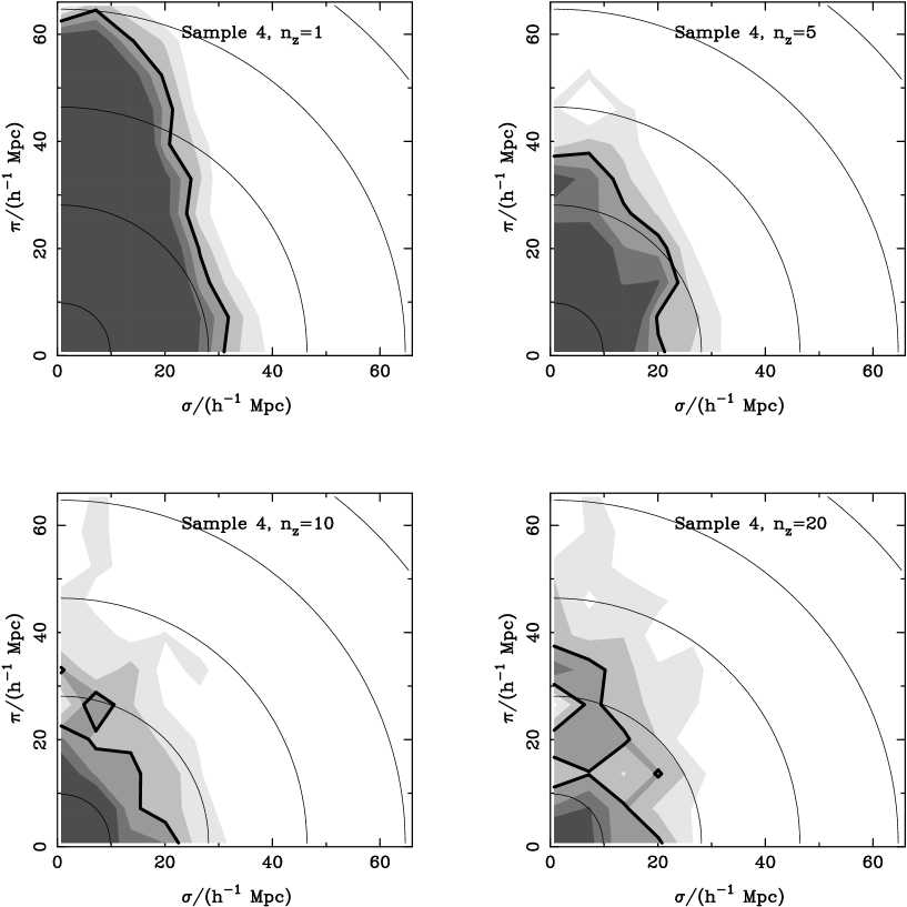
Figure 7: Correlation function results from clusters identified using mock angular data using 2D, and whose angular positions coincide with those of real clusters in the simulation (mock sample 4). Cluster distances were obtained using $1$, $5$, $10$ and $20$ redshifts (panels upper left, upper right, lower left, and lower right respectively). Shadings and line conventions are as in figure 1.

As can be seen in figure 7, the projection effects in sample 3 are still present, even after the clusters have coincident angular positions with a cluster sample identified in 3D. The elongations in $\xi(\sigma,\pi)$ are quite severe, and reflect the contamination of foreground and background structures, which introduces biases in the cluster distances.

4.3 Effects of projected radius in the identification algorithm

The algorithms used to identify clusters from angular data depend quite sensitively on the search radius $r_{c}$ used to find member candidates. In the case of Abell clusters this corresponds to $r_{c}=1.5$h^-1Mpc.

A possible cause of projection effects becomes clear when one considers that the density of galaxies diminishes as a function of cluster radius. This means that in the outskirts of the cluster, the angular population of galaxies will be composed of ever larger fractions of foreground and background galaxies. Therefore it is increasingly probable to consider as member galaxies, objects that are not physically bound to the cluster. We investigate this effect by using different cluster search radius in our 2-dimensional cluster finding algorithms. In figure 8, we show the correlation function contours for clusters identified using $r_{c}=0.5$, $1.0$ and $1.5$h^-1Mpc in the left, middle and right panels respectively. In all these cases, $n_{z}=10$, which ensures us that any elongations observed in the $\xi(\sigma,\pi)$ isopleths will be mainly produced by projection effects arising from the choice of radius.

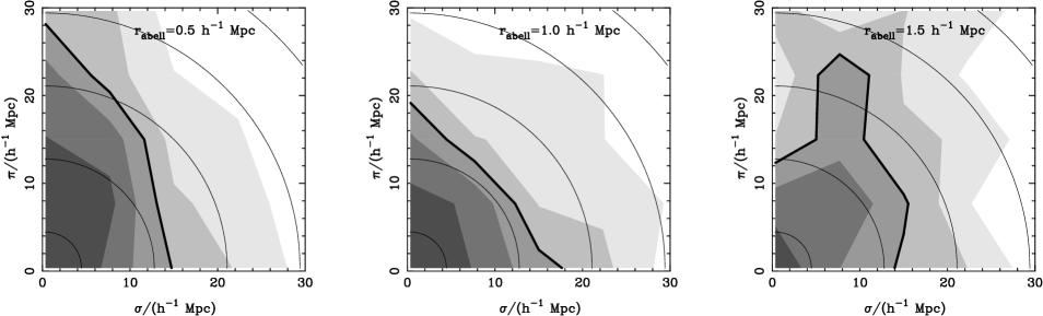
Figure 8: Correlation function contours for mock clusters identified from angular data, using $r_{c}=0.5$, $1.0$ and $1.5$h^-1Mpc in the left, middle and right hand side panels respectively. Shadings and line conventions are as in previous figures.

As can be seen, the use of a small search radius is not entirely convenient as it produces spurious clusters, probably from confusing satellite haloes with proper clusters. This is in agreement with the elongated iso-correlation contours in the left panel, and also with the small amplitude of the correlation length $\sigma_{0}$, that is $\xi(\sigma_{0},\pi=0)=1$, and is supported by figure 9, which shows the clusters of galaxies identified using $r_{c}=1.0$h^-1Mpc (circles), and those identified using $r_{c}=0.5$h^-1Mpc (dots); the gray scale of the pixels indicate number of galaxies, and the radii of the circles correspond to the radius out to which the counting of galaxies was done when finding the cluster richness. As can be seen in three cases in figure 9, the identification using a small search radius produces pairs of clusters whereas the use of a larger search radius produces a single cluster. The satellite cluster identified with a small search radius corresponds to a lower peak in the density of projected galaxies in all cases; also, the richness of a satellite is smaller than the main cluster in general, confirming the hypothesis of low mass satellites stated earlier in this paragraph.

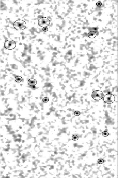
Figure 9: Clusters in mock sample 3 identified with different cluster search radius. The density of galaxies is shown as a grey-scale pixelmap. The circles show clusters identified using $r_{c}=1.0$h^-1 Mpc, and the dots, those identified using $r_{c}=0.5$h^-1 Mpc. This figure shows a sub-set of the pixelised mock galaxy catalogue and is shown in an equal area projection centred at $\alpha=1^{h}$ and $\delta=-45^{o}$, with radius $r_{eqa}=160^{o}$. The number of pixels per side is $n_{pix}=2900$, and was set in order to obtain a mean number of galaxies $n=1$ per pixel for a magnitude limit $m_{gx}<20.0$. The pixelmap sub-set size is $110{\rm x}200$ pixels.

The other values considered, $r_{c}=1.0$ and $1.5$h^-1Mpc, produce similar results, both largely free from projection effects, and with a larger correlation length $\sigma_{0}$ (figure 8). There is a slight difference in the noise level in these samples, the correlation levels in the $r_{c}=1.5$h^-1Mpc sample being less smooth than the smaller $r_{c}$ case. This is not a severe difference, but is enough to support our choice of $r_{c}=1.0$h^-1Mpc used throughout this paper.

4.4 Relative velocities and correlation lengths in mock cluster samples

Figure 10: Pairwise velocities obtained for the different samples as indicated in the legend of each panel. The different thin lines correspond to different values of $\xi(\sigma,\pi)$. The thick solid lines show the mean pairwise velocity dispersion for the full sample of clusters in the 3-dimensional simulation box.

In this section we present determinations of relative velocities, redshift-space correlation lengths and bias factor from the $\xi(\sigma,\pi)$ anisotropies. Specifically, we study the dependence of the relative pairwise peculiar velocities obtained using eq. 5 for the different mock samples as a function of $n_{z}$. We recall that the cosmological parameters of the simulation from which the mock catalogues were extracted ($\Omega_{m}=1$, $\Omega_{\Lambda}=0.0$, $\Gamma=0.21$ and $\sigma_{8}=0.6$) are those used in the calculations.

Figure 10 shows the pairwise velocities found in the different samples (sample 1 in upper left panel, sample 2 in the upper right, sample 3 in the lower left, and sample 4 in the lower right panel). The different thin lines correspond to results using different values of $\xi(\sigma,\pi)$. The thick solid line shows the mean pairwise velocity dispersion from the clusters identified in three dimensions in the simulation box.

This plot shows the great range of results which can be obtained from the contours in the correlation function if the mean $n_{z}$ used for the clusters in the sample is not known. It is remarkable the fact that the relative velocities found using clusters from sample 2 which were obtained in redshift space are in good agreement with the actual value measured from the full simulation.

The disagreement between the value of true relative cluster velocities with the measurements from the redshift-space correlations is most severe when the sample has been identified using angular data. It is also interesting that the velocities obtained from sample 4 (clusters identified from 2 dimensions with angular confirmation from inspection over the 3-dimensionally identified sample) are in some cases still very high even when their distances are obtained using a large $n_{z}$. It should be noted though, that the velocities favoured by low noise contour levels, $\xi\geq 1$, suggest small cluster relative velocities. The problem of a wide range of predictions for $w_{12}$ is not present in the case of clusters in sample 3, in part due to the larger number (almost a factor of 2) of clusters in this sample. The results obtained from different correlation levels are more compatible, showing values differing by less than $1000$ km/s among the different correlation levels. The observed behaviour of the relative velocities does not favour sample 4 over sample 3, indicating that the confirmation by angular coincidence with real clusters can not remedy the systematic problems of samples of clusters identified in two dimensions.

This problem can be dug into a little further by studying the cluster redshift-space correlation lengths, which also show great variation with $n_{z}$. We show these quantities in figure 11, where marked differences between samples of clusters identified from angular and 3-D data can be seen. Both samples obtained using 3-D information show a steady value of $s_{0}$, without any significant variation with $n_{z}$. The first important result from this figure is that the results from clusters in sample 2 are in excellent agreement with the true values. We notice that the results for sample 1 are indistinguishable from those of sample 2 and are not shown for clarity.

An interesting feature in figure 11, is the difference between confirmed and unconfirmed 2-D clusters, which also show controversial results in figure 10. The observed correlation length of clusters in sample 4 is higher than that of redshift space identified clusters in sample 2. Furthermore, this correlation length is also higher than that of the clusters in sample 3, which is expected to be more contaminated by foreground/background galaxies. This differences could be explained if several spurious clusters in sample 3, were associations of a small number of galaxies along the line of sight. The higher correlation amplitude derived for sample 4 clusters with respect to those in sample 2, could indicate that the identification of clusters using angular data is biased towards massive systems. This follows from the larger values of $s_{0}$ found from the sample of confirmed clusters. The inclusion of spurious small associations of galaxies in sample 3, would make the value of $s_{0}$ in this case smaller than those obtained for clusters in sample 2. We have also confirmed this by inspection to the mean cluster mass of samples 2 and 4.

These findings are in agreement with the results of Miller et al. (1999), who showed that by restricting a sample of Abell clusters to high richnesses the degree of projection effects is significantly reduced. The difference in correlation lengths also explains the marginally larger cluster relative velocities found in sample 4 compared with sample 3, at least when considering high levels of correlation, where the noise is not playing an important role in the results from sample 4. Equation 2 shows that the streaming velocities of clusters are proportional to their correlation functions. This means that the clusters in sample 4 have larger streaming velocities than those in sample 3. Taking into account that the elongations along the line of sight seen in figure 7 are similar for both samples, it is clear that the results from equation 5 will yield larger values of cluster relative velocities for the sample 4 than for sample 3.

Figure 11: Values of the redshift-space correlation length $s_{0}$ as a function of $n_{z}$. The symbols in these panels correspond to the different samples and are indicated in the figure. The dotted lines show the range of acceptable values as measured from the full simulation.

The results for the values of the bias parameter obtained from minimising equation 5 as a function of $n_{z}$ show a behaviour similar to the results from the redshift-space correlation length. Figure 12 shows the resulting bias parameter for the different mock samples (the symbols are indicated in the figure). The dotted lines show the acceptable range of effective bias parameters from the simulation, obtained using the Sheth, Mo & Tormen (2001) mass function, and the number density of clusters in the mock samples along with its uncertainty.

As it can be seen, the bias found for the clusters in mock sample 2 is within the acceptable values for the CDM effective bias. This result holds for any value of $n_{z}$. As in the previous figure, the results for sample 1 are consistent with the true values, and are not shown in order to preserve clarity. The result from sample 3 is in agreement for roughly $n_{z}>10$. Sample 4 shows significantly larger values of bias and correlation length, suggesting that this sample comprises a high mass cluster population in agreement with the results found earlier in this section.

Figure 12: Values of the bias parameter obtained from minimising equation 5 as a function of $n_{z}$. The symbols in these panels correspond to the different samples and are indicated in the figure. The dotted lines show the acceptable range of bias parameters for the number density of clusters in the mock samples obtained using the Sheth, Mo & Tormen (2001) mass function.

5 Conclusions

We have analysed the consequences of different effects on the distortion of the correlation function of clusters in redshift space for different mock samples of galaxy clusters. We take into account the pairwise velocity distribution of galaxy systems, coherent bulk motions, as well as redshift errors, and different cluster identification systematics. The mock cluster samples were extracted from numerical simulations, following algorithms that closely match the procedures used to identify the clusters in observational samples. We find that the correlation function of galaxy systems is influenced by wrongly assigned cluster distances due to a small number of galaxy redshift measurements in the fields of clusters. However, the most important effect is that associated with the cluster identification procedure from two dimensional surveys. Due to these effects, the estimated mean pairwise velocity dispersion can be an order of magnitude larger than the actual value.

This is consistent with the observed anisotropy of the correlation function contours of UZC groups, which shows the flattening produced by this infall motion (Padilla et al. 2001). For samples of clusters identified in mock galaxy redshift surveys we find an infalling pattern even in the case where the distances to groups or clusters of galaxies are obtained using a small number of member redshifts.

Figure 13: Correlation function results from mock 2dF100k release galaxy groups constructed by Merchán & Zandivarez (2002). Shadings and line conventions are as in figure 1.

In order to provide predictions for new generation cluster catalogues we have also analysed a mock sample of groups resembling those obtained by Merchán & Zandivarez (2002) from the 2dF100K release galaxy redshift survey. This mock catalogue is subject to the same complicated angular mask as the observations and serves as a further test of the reliability of the information that can be obtained from observational cluster and group catalogues. The results shown in figure 13 are similar to those of Sample 2, and indicate that the angular mask does not affect severely the results so that consistent values of $w_{12}$ and $s_{0}$ can be derived.

In order to explore the projection effects afflicting cluster samples identified in two dimensions we analysed different mock cluster samples identified from mock angular catalogues using different cluster search radius. Our findings favour the use of smaller radius than that used in the identification of Abell clusters. The use of a too small value produces a sample increasingly affected by projection effects and the inclusion of smaller groups of galaxies which are probably cluster satellite haloes.

We notice that 2-dim identified clusters whose angular positions coincide with a true 3-dim cluster show a strongly distorted clustering pattern. This fact shows the large influence of groups and clusters along the line of sight in the observed elongation. Contamination is therefore mainly arising from structures present in the filamentary large scale distribution. These results indicate the difficulties of obtaining unbiased cluster samples even when using accurate photometric data such as present in new and forthcoming surveys. Redshift information is crucial for constructing cluster samples which lack significant projection effects, since galaxy colours alone can remove foreground and background contamination but not distinguish membership to clusters at relatively smaller separations along the line of sight.

References

- [] Abadi, M.G., Lambas, D.G., Muriel, H., 1998, ApJ, 507, 526.
- [] Bahcall, N.A., Cen, R.Y., 1992, ApJ, 398, L81.
- [] Bahcall, N.A., Cen, R.Y., Gramann, M., 1994, ApJ, 430, L13.
- [] Bahcall, N.A., Soneira, R.M., 1983, ApJ, 270, 20.
- [] Bahcall, N.A., Soneira, R.M., Burgett, W.S., 1986, ApJ, 311, 15.
- [] Baugh, C.M., 1996, MNRAS, 280, 267.
- [] Bean, A.J., Efstathiou, G., Ellis, R.S., Peterson, B.A., Shanks, T., 1983, MNRAS, 205, 605.
- [] Borgani, S., Plionis, M., Kolokotronis, V., 1999, MNRAS, 305, 866.
- [] Colberg, J.M., et al. , 2000, MNRAS, 319, 209.
- [] Cole, S., Hatton, S.J., Weinberg, D.H., Frenk, C.S., 1998, MNRAS, 300, 945.
- [] Collins, C.A., Guzzo, L., Boehringer, H., Schuecker, P, Chincarini, G., Cruddace, R., De Grandi, S, MacGillivray, H.T., Neumann, D.M., Schindler, S., Shaver, P., Voges, W., 2000, MNRAS, 319, 939.
- [] Croft, R.A.C., Efstathiou, G., 1994a, MNRAS, 268, L23.
- [] Croft, R.A.C., Efstathiou, G., 1994b, MNRAS, 267, 390.
- [] Croft, R.A.C., Dalton, G.B., Efstathiou, G., Sutherland, W.J., Maddox, S.J., 1997, MNRAS, 291, 305.
- [] Dalton, G.B., Efstathiou, G., Maddox, S.J., Sutherland, W.J., 1992, ApJ, 390, L1.
- [] Dalton, G.B., Efstathiou, G., Maddox, S.J., Sutherland, W.J., 1994, MNRAS, 269, 151.
- [] Dalton, G.B., Maddox, S.J., Sutherland, W.J., Efstathiou, G., 1997, MNRAS, 289, 263.
- [] Davis, M., & Peebles, P.J.E., 1983, ApJ, 267, 465.
- [] Ebeling, H.; Voges, W.; Bohringer, H.; Edge, A. C.; Huchra, J. P.; Briel, U. G., 1996, MNRAS, 281, 799.
- [] Eke, V.R., Cole, S., Frenk, C.S., Navarro, J.F., 1996, MNRAS, 281, 703.
- [] Evrard, A. E.; MacFarland, T. J.; Couchman, H. M. P.; Colberg, J. M.; Yoshida, N.; White, S. D. M.; Jenkins, A.; Frenk, C. S.; Pearce, F. R.; Peacock, J. A.; Thomas, P. A. 2002, ApJ, 573, 7.
- [] Governato, F., Babul, A., Quinn, T., Tozzi, P., Baugh, C.M., Katz, N., Lake, G., 1999, MNRAS, 307, 949.
- [] Hamilton, A., 1993, ApJ, 417, 19.
- [] Helly, J.C., Cole, S., Frenk, C.S., Baugh, C.M., Benson, A., & Lacey, C., 2002, accepted for publication in MNRAS, astro-ph/0210141.
- [] Huchra, J.P., & Geller, M.J., 1982, ApJ, 256, 423.
- [] Jenkins, A., Frenk, C.S., White, S.D.M., Colberg, J.M., Cole, S., Evrard, A.E., Couchman, H.M.P., Yoshida, N., 2001, MNRAS, 321, 372.
- [] Loveday, J., Efstathiou, G., Maddox, S.J., & Peterson, B.A., 1996, ApJ, 468, 1.
- [] Lucey, J. R., 1983, MNRAS, 204, 33.
- [] Lumsden, S.L., Nichol, R.C., Collins, C.A., Guzzo, L., 1992, MNRAS, 258, 1.
- [] Merchán, M., & Zandivarez, A., 2002, MNRAS, 335, 216.
- [] Miller, C.J., Batuski, D.J., Slingend, K.A., Hill, J.M., 1999, ApJ, 523, 492.
- [] Norberg,P. et al., 2002, MNRAS, 332, 827.
- [] Padilla, N.D., & Lambas, D.G., 2003, MNRAS, submitted.
- [] Padilla, N.D., & Baugh, C.M., 2002, MNRAS, 329, 431.
- [] Padilla, N.D., Merchan, M.E., Valotto, C.A., Lambas, D.G., Maia, M.A.G., 2001, ApJ, 554, 873.
- [] Peacock, J. A. & West, M.J., 1992, MNRAS, 259, 494.
- [] Peacock et al. 2001, defi.conf, 221.
- [] Postman, M., Huchra, J.P., Geller, M.J., 1992, ApJ, 384, 404.
- [] Ratcliffe, A., Shanks, T., Parker, Q.A., & Fong, R. 1998, MNRAS, 296, 191.
- [] Sheth, R.K., Mo, H.J., Tormen, G., 2001, MNRAS, 323, 1
- [] Sutherland, W., 1988, MNRAS, 234, 159.
- [] Sutherland, W.J., Efstathiou, G., 1991, MNRAS, 248, 159.
- [] van Haarlem, M.P., Frenk, C.S., White, S.D.M., MNRAS, 1997, 287, 817.
- [] Watanabe, T., Matsubara, T., Suto, Y., 1994, ApJ, 432, 17.
- [] White, S.D.M., Frenk, C.S., Davis, M., Efstathiou, G., 1987, ApJ, 313, 505.