Roche tomography of cataclysmic variables – II. Images of the secondary stars in AM Her, QQ Vul, IP Peg and HU Aqr

Abstract

We present a set of Roche tomography reconstructions of the secondary stars in the cataclysmic variables AM Her, QQ Vul, IP Peg and HU Aqr. The image reconstructions show distinct asymmetries in the irradiation pattern for all four systems which can be attributed to shielding of the secondary star by the accretion stream/column in AM Her, QQ Vul and HU Aqr, and increased irradiation by the bright spot in IP Peg. We use the entropy landscape technique to derive accurate system parameters ($M{{}_{1}}$, $M_{2}$, $i$ and $\gamma$) for the four binaries. In principle, this technique should provide the most reliable mass determinations available, since the intensity distribution across the secondary star is known. We also find that the intensity distribution can systematically affect the value of $\gamma$ derived from circular orbit fits to radial velocity variations.

1 Introduction

The secondary, Roche-lobe-filling stars in CVs are key to our understanding of the origin, evolution and behaviour of this class of interacting binary. To best study the secondary stars in CVs, we would ideally like direct images of the stellar surface. This is currently impossible, however, as typical CV secondary stars have radii of 400 000 km and distances of 200 pc, which means that to detect a feature covering 20 per cent of the star’s surface requires a resolution of approximately 1 microarcsecond, 10 000 times greater than the diffraction-limited resolution of the world’s largest telescopes. Rutten & Dhillon (1994) and Watson & Dhillon (2001, hereafter referred to as Paper I) described a way around this problem using an indirect imaging technique called Roche tomography which uses phase-resolved spectra to reconstruct the line intensity distribution on the surface of the secondary star.

Obtaining surface images of the secondary star in CVs has far-reaching implications. For example, a knowledge of the irradiation pattern on the inner hemisphere of the secondary star in CVs is essential if one is to calculate stellar masses accurately enough to test binary star evolution models (see Smith & Dhillon 1998). Furthermore, the irradiation pattern provides information on the geometry of the accreting structures around the white dwarf (see Smith 1995).

In this paper we present new Roche tomograms of the secondary star in the dwarf nova IP Peg, and the magnetic CVs AM Her and QQ Vul in the light of the Na I $\lambda\lambda$8183,8195 Å absorption doublet. In addition, we also present a Roche tomogram of the magnetic CV HU Aqr in the light of the He II $\lambda$4686 Å emission line component known to originate from the secondary star. These tomograms allow a study of the irradiation pattern on the secondary stars as well as providing measurements of the binary parameters for all four CVs.

2 Observations and reduction

The spectra of QQ Vul and HU Aqr were taken on the 3.5-m telescope at Calar Alto and full details of the observations and subsequent data reduction can be found in Catalán, Schwope & Smith (1999) and Schwope, Mantel & Horne (1997), respectively.

The observations of IP Peg and AM Her were carried out over two nights on 1994 August 11–12 using the ISIS dual-beam spectrograph and 1200 lines mm^-1 gratings on the 4.2m William Herschel Telescope (WHT). The EEV3 CCD chip in the red arm covered the wavelength range 7985–8437Å at a resolution of 0.37Å  ($\sim$27 km s^-1). The TEK2 CCD chip on the blue arm covered the wavelength range 4560–4968Å  at a resolution of 0.4Å ($\sim$50 km s^-1). To reduce readout noise, the pixels were binned by a factor of 2 in the spatial direction. Each object was observed using exposure times of 300 seconds and a nearby field star was located on the slit to correct for slit losses. Wide slit spectra of the companion star were also taken to permit absolute spectrophotometry. Sky-flats and tungsten flats were taken on both nights and a CuAr+CuNe arc spectrum was taken approximately every 50 minutes in order to wavelength calibrate the spectra. Narrow and wide slit spectra at a range of different air-masses were taken of flux standards for the purposes of flux calibration and water removal. We also observed a range of M-dwarf spectral-type templates in order to obtain a Na I intrinsic line profile for use in Roche tomography.

During the reduction process, bias subtraction, division by a master flat-field frame and sky subtraction were carried out and then the spectra were optimally extracted (Horne, 1986). The arc spectra were used to wavelength calibrate the data, with an rms error of 0.01Å. Slit loss correction was then applied by dividing the object spectra by the average value per pixel (after masking out strong lines, cosmic rays and telluric features) in the corresponding comparison star spectra, and later multiplying by the average value per pixel in the wide-slit comparison star spectrum. Telluric absorption and absolute flux calibration were then performed using the standard star spectra.

In total we obtained 79 spectra of IP Peg and 51 spectra of AM Her. We present only the red spectra in this paper, as we are only concerned with the Na I doublet at $\lambda\lambda$8183,8195Å  for the purposes of this work. A full journal of observations is presented in Table LABEL:tab:journal.

Table 1: Journal of observations. Orbital phase is shown for AM Her using the ephemeris of Southwell et al. (1995), and IP Peg using the ephemeris of Wolf et al. (1993). Since the latter ephemeris is deduced from the white-dwarf egress in IP Peg, an appropriate correction has been made to ensure that phase 0 corresponds to the superior conjunction of the primary. Note: HU Aqr was trailed along the slit during the exposures. The final time resolution was $\sim$ 30 s, and the data was phase-folded into 100 phase bins covering a complete orbital cycle.

Object	UT Date	UT	UT	Phase	Phase	$T_{\exp}$	No. of
	(D/M/Y)	start	end	start	end	(s)	Spectra
AM Her	11/08/94	21:38	23:58	0.57	1.29	300	22
AM Her	12-13/08/94	21:20	00:09	2.22	3.11	300	29
QQ Vul	08-09/07/91	23:33	04:10	0.12	1.33	345–720	16
QQ Vul	09-10/07/91	21:47	03:52	6.12	7.71	600–680	20
IP Peg	12/08/94	01:23	05:26	0.88	1.93	300	41
IP Peg	13/08/94	01:13	05:11	7.16	8.18	300	38
HU Aqr	17-18/08/93					750–1800	7

3 Roche tomography

3.1 Techniques

Roche tomography (Rutten & Dhillon 1994; Dhillon & Watson 2001; Paper I) is analogous to the Doppler imaging technique used to map rapidly rotating single stars (e.g. Vogt & Penrod 1983). In Roche tomography the secondary star is assumed to be Roche-lobe-filling, locked in synchronous rotation and to have a circularized orbit. The secondary star is then modelled as a series of quadrilateral tiles or surface elements, each of which is assigned a copy of the local (intrinsic) specific intensity profile. These profiles are then scaled to take into account the projected area of the surface element, limb darkening and obscuration, and then Doppler shifted according to the radial velocity of the surface element at that particular phase. Summing up the contributions from each element gives the rotationally broadened profile at that particular orbital phase.

By iteratively varying the strengths of the profile contributed from each element, the ‘inverse’ of the above procedure can be performed. Due to the variable and unknown contribution to the spectrum of the accretion regions in CVs, the data must be slit-loss corrected and continuum subtracted prior to mapping with Roche tomography. Thus, Roche tomograms present images of the distribution of line flux on the secondary star. The data is fit to an aim $\chi^{2}$, and a unique map is selected by employing the maximum entropy (MEMSYS) algorithm developed by Skilling & Bryan (1984). The definition of image entropy, $S$, that we use is

$$S=\sum_{j=1}^{k}m_{j}-d_{j}-m_{j}\ln\left(m_{j}/d_{j}\right)$$

where $k$ is the number of tiles in the map, and $m_{j}$ and $d_{j}$ are the map of line flux and the default map, respectively. We employ a moving uniform default map, where each element in the default is set to the average value in the map. For further details of the Roche tomography process see the review by Dhillon & Watson (2001).

For those CVs where we wish to map the Na I doublet, Roche tomography requires the intrinsic line profile to be input as a template. Ideally, this should be the same line taken from the spectrum of a slowly rotating star of the same spectral class as the star being mapped, preferably obtained with the same instrumental set-up. Unfortunately, only one of the spectral-type template stars that were observed is useful (GL806 – see Table LABEL:tab:templates); the others show signs of broadening of the Na I doublet and have been identified as either flare stars, and are therefore probably rapidly rotating, or binary stars, where $V_{rot}\sin i$ measurements using the Na I absorption doublet have been found to be systematically greater than those given by the narrow metal lines (Bleach et al. 2000). We used the GL806 template in all of our reconstructions and, even though the spectral class of the template differs from those of the stars being mapped, the exact shape of the template profile used has little effect on the reconstructions due to the large degree of rotational broadening present in CV secondary stars.

For the CVs mapped using the Na I doublet, it is necessary to correct the derived systemic velocities for the systemic velocity of the spectral-type template used in the reconstructions. The systemic velocity of GL806 was determined by fitting gaussians to the Na I doublet, which yielded a value of $\gamma$ = –24.3 $\pm$ 1.1 km s^-1. For comparison, Wilson (1953) found the systemic velocity of GL806 to be –15 $\pm$ 5 km s^-1, whereas Gliese (1969) quote a value of –24.4 km s^-1.

It is important to note that the maximum-entropy algorithm we use requires that the input data are positive. As a result, it is necessary to invert absorption-line profiles and, in the case of low signal-to-noise data, add a positive constant in order to ensure that there are no negative values in the continuum-subtracted data. If this positive constant is not added, and any negative points are either set to zero or ignored during the reconstruction, then the fit will be positively biased in the wings of the line profile wings. The exact value of this constant is unimportant, so long as it prevents the occurrence of negative values in the data and is effectively removed. We account for this positive constant during the reconstruction by employing a virtual image element which contributes a single value to all data points, effectively cancelling out the constant. For the systems where the Na I doublet has been used in the reconstructions, we have employed this technique of adding a positive constant to each data value. We find that this significantly improves the reliability of the technique to determine the component masses when noisy data are being used. As the data for HU Aqr are from Gaussian fits to the He II $\lambda$4686Å  emission line, there are no errors in the continuum and hence we do not apply this technique.

In addition, we have accounted for the effects of velocity smearing due to the motion of the secondary star over the duration of an exposure for all four systems. This is done by calculating the profile at evenly spaced intervals over one exposure and then averaging them. Although computationally more time-consuming, this reduces the effects of smearing, and can also take into account features that may cross the limb of the secondary star during an exposure.

3.2 Determining the system parameters

Roche tomograms are greatly influenced by parameters such as the component masses, inclination and systemic velocity of the binary. Errors in the assumed values of these parameters degrades the quality of the surface map and, in general, results in additional structure in the Roche tomograms. The correct parameters are, therefore, those that produce the map containing the least artefacts, corresponding to the map of highest entropy (Paper I). By carrying out reconstructions for many pairs of component masses (iterating to the same $\chi^{2}$ on each occasion) we can construct an ‘entropy landscape’ (e.g., Fig. 3), where each point corresponds to the entropy value obtained in a reconstruction for a particular pair of component masses.

In order to determine the binary parameters of the CVs studied in this paper, we constructed a series of entropy landscapes assuming a wide range of different values for the orbital inclination and systemic velocity. For each combination of $i$ and $\gamma$, we picked the maximum entropy value in the corresponding entropy landscape, and plotted this value in the $i-\gamma$ plane, which is shown for each object on the left-hand side of Fig. 1. In all cases we found that a unique or optimal systemic velocity could be selected that consistently gave the map of maximum entropy. In addition, the value of the optimal systemic velocity was found to be largely independent of the orbital inclination assumed during the reconstructions, as demonstrated in the left-hand plots of Fig. 1. For example, in reconstructions carried out over a range of inclinations spanning 30^∘, the systemic velocity we obtain for both IP Peg and AM Her only varies by 1 km s^-1.

The inclination, however, is not as well constrained for any of the CVs. The right-hand plots on Fig. 1 show cuts through the plots in the $i-\gamma$ plane at the optimal systemic velocity, and the scatter clearly demonstrates the difficulty in selecting an optimal inclination, although the deterioration in the quality of the reconstruction for some inclinations allow limits to be set.

Table 2: Spectral-type templates observed with the WHT.

Object	Spec. Type	Notes
GL 65B	M5.5V	flare star
GL 866	M5.5V	flare star
GL 83.1A	M4.5V	flare star
GL 699	M4Ve	variable star
GL 725A	M3V	double star
GL 806	M1.5V	used in this paper

The difficulty in constraining the inclination can be explained by considering that there are two ways of determining the inclination of non-eclipsing CVs from the spectra of the secondary star alone. First, from the variation in the projected radius of the Roche-lobe shaped secondary star as it is viewed at different aspects, corresponding to a variation in the shape (or measured $v\sin i$) of the line profiles (see Shahbaz 1998). The second is from the variation in the strength of the profiles, since a high inclination system will exhibit a much greater variation in the line profile strength than a low inclination system with the same surface intensity distribution.

Unfortunately, the variation in $v\sin i$ is expected to be, at most, around 20–25 km s^-1 for high inclination systems. Although this is comparable to the velocity resolution of our data, it is buried in noise and hence the mapping technique is largely blind to any such variations. Our only constraint on the inclination, therefore, comes from the variation of the line strength, which also has its limitations. Although, rapidly varying features can only be mapped onto high inclination systems, slowly varying features produced by a low inclination system can also be mapped onto the polar regions of a high inclination system with little loss in the quality of the reconstruction. Thus we only expect to constrain the inclination in CVs which have high inclinations and exhibit strong asymmetries in their surface intensity distributions. In addition, for the same reason outlined above, we also expect our determinations to be biased towards higher inclinations.

As we cannot reliably constrain the inclination of the non-eclipsing CVs in this work, and hence the component masses, Fig. 2 shows the derived component masses as a function of inclination. The top section of each panel in Fig. 2 also shows the mass ratio derived for each inclination. Since $v\sin i$ is purely a function of the mass ratio $q$ (=$M_{1}/M_{2}$) and the radial velocity semi-amplitude of the secondary star $K_{r}$, reconstructions over a range of inclinations should yield the same value of the mass ratio on each occasion. This is confirmed in Fig. 2, with the scatter in the values serving as an indication of the noise in the technique. Indeed, the scatter can be accounted for by the fact that the component masses are only varied in 0.02M_⊙ increments in the entropy landscapes.

Entropy landscapes representative of the mass estimates for each system are shown in Fig. 3, and a summary of the adopted system parameters can be found in Table LABEL:tab:estimates. The results for each CV are discussed in more detail in the relevant sections below.

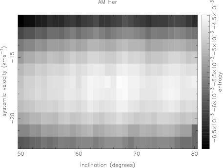
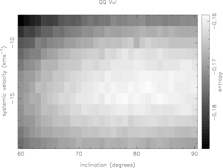
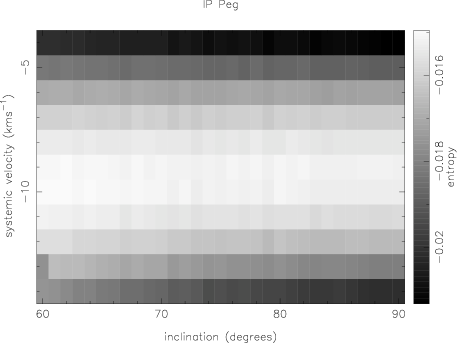
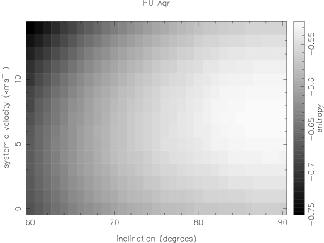
Figure 1: The plots on the left show the maximum entropy value obtained in each entropy landscape when a particular combination of inclination and systemic velocity is employed during the reconstructions; horizontal cuts through these plots at the optimal systemic velocity found for each object are shown on the right. From top to bottom: AM Her, QQ Vul, IP Peg and HU Aqr. The solid curves show parabolic fits to the data points.

Figure 2: Estimates of the component masses for different inclinations. Clockwise from top left: AM Her, QQ Vul, HU Aqr and IP Peg. The top panel of each plot shows the mass ratio, the lower panel shows the individual masses with the upper curve showing the primary mass and the lower curve showing the secondary mass.

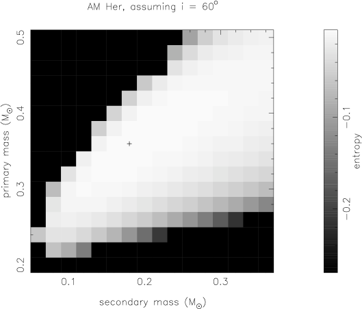
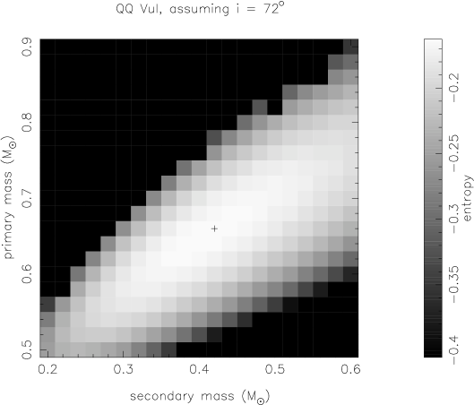
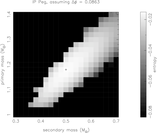
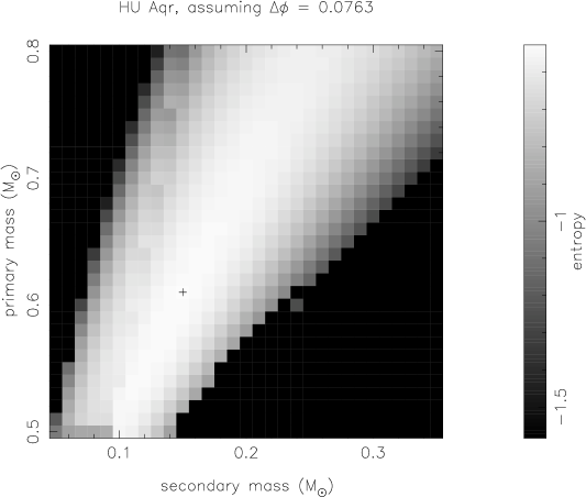
Figure 3: Entropy landscapes for the four CVs. Clockwise from top left: AM Her, QQ Vul, HU Aqr and IP Peg. Dark regions indicate masses for which no acceptable fit could be found. The cross marks the point of maximum entropy in each landscape.

Table 3: Adopted system parameters.

	AM Her	QQ Vul	IP Peg	HU Aqr
$i$	60–80∘	72${}^{\circ}\leq$ i $\leq$90∘	82∘– 85∘	84.4∘
$q$	0.53	0.63	0.43	0.25
$M_{1}$ ($M_{\odot}$)	$\sim$0.36	0.58–0.66	1.16–1.18	0.61
$M_{2}$ ($M_{\odot}$)	$\sim$0.18	0.34–0.44	0.50	0.15
$\gamma$ (km s-1)	–17	–14	–9	+7

4 Results for AM Her

4.1 The binary geometry of AM Her

From Fig. 1 the maximum entropy value yields a value of –17 km s^-1 for the systemic velocity of AM Her, taking into account the systemic velocity of the template star. This is within 2$\sigma$ of the range of values found by Young, Schneider & Shectman (1981) of –14 $\pm$ 4 km s^-1 and –40 $\pm$ 15 km s^-1 from circular fits to the H$\gamma$ and He I $\lambda$4471Å emission lines, respectively.

Fig. 1 also shows the maximum entropy value as a function of inclination obtained in entropy landscapes constructed assuming an optimum systemic velocity of –17 km s^-1. It appears as though we cannot determine a unique inclination for AM Her, though our work suggests that the inclination may lie around 60–80^∘. Given that we expect our results to be biased towards higher inclinations, the inclination is most likely to be around 60^∘. Although this estimate is far greater than the $\sim$35^∘ determined by Brainerd & Lamb (1985), it is consistent with the findings of Davey & Smith (1996) who used radial-velocity curve fitting to constrain the inclination to be between 45^∘ and 60^∘. Greeley et al. (1999) observed a partial eclipse of the He II $\lambda$1640 Å emission line region by the secondary star and hence inferred an inclination $\geq$45^∘. In addition to this, Wickramasinghe et al. (1991) obtained $i=52^{\circ}$ from polarimetric observations.

Fig. 3 shows the entropy landscape for AM Her constructed using $i$ = 60^∘, $\gamma$ = –17 km s^-1 and taking into account velocity smearing introduced by the 300 second exposure times. The brightest point on this plot indicates the map of highest entropy, and corresponds to $M_{1}$ = 0.36 M_⊙ and $M_{2}$ = 0.18 M_⊙, which we adopt as our best estimate of the component masses. The optimum component masses decrease to $M_{1}$ = 0.24 M_⊙ and $M_{2}$ = 0.12 M_⊙ for $i$ = 80^∘. These masses appear suspiciously low since AM Her lies above the period gap and we would not, therefore, expect the secondary mass to be significantly less than $M_{2}$ = $\sim$0.25 M_⊙. This partly confirms our speculation that our inclination determinations are biased towards high inclinations (Section 3.2) and that the inclination is not likely to be greater than 60^∘.

The mass of the secondary star derived from the entropy landscape agrees well with the value of $M_{2}$ = 0.20 – 0.26 M_⊙ estimated by Southwell et al. (1995). This also agrees with the main-sequence mass-period relation derived by Smith & Dhillon (1998), which gives a secondary star mass of 0.23$\pm$0.02 M_⊙.

Meaningful comparison of the primary mass derived in our work with other published white dwarf masses is, unfortunately, more difficult as they cover a wide range of values, including: 0.39 M_⊙ (Young et al., 1981), 0.69 M_⊙ (Wu, Chanmugam & Shaviv, 1995), 0.75 M_⊙ (Mukai & Charles, 1987), 0.91 M_⊙ (Mouchet, 1993) and 1.22 M_⊙ (Cropper, Ramsay & Wu, 1998). Gänsicke et al. (1998), however, concluded that the white dwarf mass in AM Her was between 0.35 – 0.53 M_⊙ and ruled out a white dwarf mass as high as 1.22 M_⊙. In addition to their secondary star mass estimate, Southwell et al. (1995) derived $q$ = 0.47$\pm$0.08, in agreement with the value of $q$ = 0.53 obtained in this work (Fig. 2).

4.2 The surface map of AM Her

The Roche tomogram for AM Her is presented in Fig. 4 and shows a decrease in the amount of Na I absorption around the inner Lagrangian ($L_{1}$) point on the trailing hemisphere. We tested the significance of this feature using the following procedure:

1. Fit the ‘true’ map using the observed data (Fig. 4).

2. Compute 200 ‘trial’ maps from simulated data sets constructed using bootstrap re-sampling. From our observed trailed spectrum containing $n$ data points we formed a simulated trailed spectrum by selecting, at random and with replacement, $n$ data values and placing these at their original positions in the new simulated trailed spectrum. For points that are not selected, the associated error bar was set to infinity and hence they were effectively omitted from the fit. For points selected more than once, the error bars were divided by the square root of the number of times they were picked (see Paper I for more details).

3. Calculate 200 ‘difference’ maps by subtracting each ‘trial’ map from the ‘true’ map. These ‘difference’ maps give the scatter in each pixel. (It would be incorrect to now calculate a summary error statistic like the standard deviation, as the distribution of pixel values is often found to be non-normal; see Paper I).

4. Subtract some mean or comparison level from the ‘true’ map. For instance, if one wished to determine the significance of a starspot, an appropriate comparison level to subtract from the ‘true’ map would be a region of immaculate photosphere. Subtract the corresponding level from each of the ‘difference’ or ‘scatter’ maps.

5. Rank each pixel in the ‘true’ map computed in step (iv) against the corresponding pixel in the ‘scatter’ maps. This will show the fraction of fluctuation values that the observed value in the ‘true’ map exceeds.

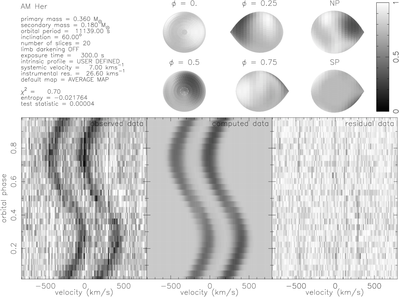
Figure 4: Roche tomogram of AM Her. Bright greyscales in the tomograms depict regions of enhanced Na I absorption. The greyscales are reversed in the trailed spectra. Note that the systemic velocity quoted in the upper-left of the panel does not take into account the systemic velocity of the spectral-type template star.

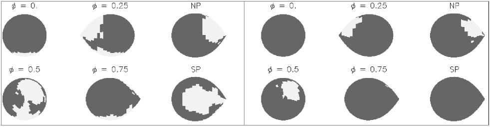
Figure 5: Significance maps of AM Her. The four images on the left-hand side of each panel are viewed in the equatorial plane, and the two images on the right-hand side of each panel are viewed from above and below the north and south pole respectively. The significance map in the left-hand panel was constructed by taking the comparison level to be the average intensity of the outer hemisphere. The significance map in the right-hand panel was constructed by taking the comparison level to be the average intensity of the region around the $L_{1}$ point that does not appear to be irradiated. Bright greyscales indicate regions where the ‘true’ map ranks above 100 per cent of the ‘scatter’ maps. The significance of the region near the south pole (SP) in the left-hand panel is an artefact, since this region is never observed.

For our first test we took the average intensity of the outer (and presumably non-irradiated) hemisphere of the star as our comparison level, thereby testing the reality of the asymmetry between the outer and inner hemispheres. The left-hand panel in Fig. 5 shows the resultant significance map, calculated using the procedure listed above. The bright greyscale depicts regions where the ‘true’ map ranks above 100 per cent of the ‘scatter’ maps, and therefore represents regions where the intensity is significantly different from the outer hemisphere. Dark greyscales represent regions of the map that do not rank highly against the scatter map. Features in these regions are not, therefore, significantly different from the average intensity of the outer hemisphere.

The left-hand panel in Fig. 5 shows that the irradiation seen on the inner hemisphere in the Roche tomogram is real, and appears more significant on the trailing hemisphere (i.e., $\phi$ = 0.25). Note that the significance of the regions near the south pole (SP) is an artefact. Due to the inclination of AM Her, latitudes $>i$ in the southern hemisphere are never seen and hence the reconstructions always assume the (same) default level, with very little scatter in the intensity values. As a result, regions near the south pole will appear significantly different from the comparison level unless, of course, the comparison level is very similar to the default level.

The right-hand panel in Fig. 5 shows another significance map, but taking the comparison level as a region around the $L_{1}$ point on the leading hemisphere ($\phi$ = 0.25). This shows that the asymmetry between the leading and trailing hemispheres is real, and that the effects of irradiation are primarily found on the trailing hemisphere. The asymmetry in the irradiation pattern between the northern and southern hemisphere is again an artefact, since regions on the southern hemisphere are less visible and the data does not constrain the reconstructions in these regions. Note that in this case, the comparison level selected was similar to the default level of the map, and therefore regions near the south pole (SP) no longer appear to be significant.

Our results are in agreement with the surface maps of AM Her obtained using the method of radial-velocity curve fitting (Davey & Smith 1992, 1996). They proposed that the lack of irradiation on the leading hemisphere could be explained if the incoming accretion column was able to block the radiation produced close to the white dwarf and found that the accretion geometry given by Cropper (1988) supported this argument.

5 Results for QQ Vul

5.1 The binary geometry of QQ Vul

The systemic velocity and inclination of QQ Vul were determined in the manner outlined in Section 3.2, and the results are shown in Fig. 1. We find that the systemic velocity is well constrained with a value of –14 km s^-1, comparable with the value of 17 $\pm$ 23 km s^-1 obtained by Mukai & Charles (1987). Catalán et al. (1999) found $\gamma$ = –0.2 $\pm$ 2.2 km s^-1 from the results of elliptical fits to the Na I absorption lines used in this work. In addition, using the same method they also obtained $\gamma$ = –8.3 $\pm$ 1.6 km s^-1 using data obtained on the WHT in 1993. One explanation for this difference in the systemic velocity is if a change in the intensity distribution between the two epochs can alter the measured value of $\gamma$ (we explore this possibility in Section 7).

It is clear from Fig. 1 that it is difficult to select a single value for the inclination given the scatter in the distribution of the points. The quality of the reconstructions does, however, begin to deteriorate towards lower inclinations allowing us to set a lower of limit of $\sim$72^∘ for the inclination of QQ Vul.

Previous estimates of the orbital inclination include $i$ = 50^∘–70^∘ (Schwope et al., 2000), $i$ = 65${}^{\circ}\pm$7^∘ (Catalán et al., 1999), $i$ = 60${}^{\circ}\pm$ 14^∘ (Mukai & Charles, 1987) and 46${}^{\circ}<i<$ 74^∘ (Nousek et al., 1984). In addition, Nousek et al. (1984) also found evidence of a brief eclipse of the cyclotron region combined with the simultaneous disappearance of emission lines. They attributed this to an eclipse by the secondary star, forcing the orbital inclination to the upper limit of 46${}^{\circ}<i<$ 74^∘. From EUVE observations Belle, Howell & Mills (2000) also suggested that the X-ray emitting region is eclipsed by the secondary star, constraining the inclination to $>$ 60^∘. Certainly, in this work we can rule out inclinations $<$ 60^∘ due to the low entropy of the reconstructions at these inclinations. These claims of eclipse features, however, are outside phase 0 and thus cannot be attributed to the secondary star. The lack of an X-ray eclipse at this phase means that an inclination $>$ 72^∘ can be excluded.

Fig. 3 shows the entropy landscape for QQ Vul, constructed assuming an inclination of 72^∘, from which we derive optimum masses of $M_{1}$ = 0.66 M_⊙ and $M_{2}$ = 0.42 M_⊙. We adopt these masses and inclination for the reconstruction in Section 5.2. The derived masses, however, decrease smoothly as the inclination is increased to 90^∘ and cover the range $M_{1}$ = 0.58–0.66 M_⊙, $M_{2}$ = 0.34–0.44 M_⊙ at a constant $q$ = 0.63. This agrees well with, and is better constrained than, the masses of $M_{1}$ = 0.54${}^{+0.21}_{-0.16}$ M_⊙ and $M_{2}$ = 0.30$\pm$0.10 M_⊙ estimated by Catalán et al. (1999).

The white-dwarf mass we derive agrees with the values of $M_{1}$ = 0.58${}^{+0.44}_{-0.09}$ M_⊙ (Mukai & Charles, 1987) and $M_{1}$ = 0.59 M_⊙ (Mouchet, 1993), but is almost half that of Cropper et al. (1998) and Wu et al. (1995) who obtained $M_{1}$ = 1.22 M_⊙ and $M_{1}$ = 1.1–1.3 M_⊙, respectively. The two latter mass determinations make use of the X-rays emitted from the accreting white dwarf and involve fitting model spectra to the observed X-ray spectra, and are therefore subject to underlying assumptions in the model.

The mass ratio of $q$ = 0.63 obtained in this work is in excellent agreement with previous determinations, including $q$ = 0.54$\pm$0.14 (Catalán et al., 1999) and $q$ = 0.45–0.67 determined by Schwope et al. (2000) from Doppler tomography and polarimetry.

5.2 The surface map of QQ Vul

The Roche tomogram of QQ Vul is presented in Fig. 6 and shows a distinct reduction in the Na I absorption around the $L_{1}$ point which can be explained by irradiation from the white dwarf and accretion regions ionising the Na I on the inner face of the secondary, as in AM Her. The effects of irradiation also appear to be slightly stronger on the trailing hemisphere, suggesting that the leading hemisphere may be partially shielded by the accretion stream or curtain.

Another notable feature is a bright patch on the leading hemisphere, corresponding to an increased Na I flux deficit around phase 0.75. A similar feature can also be seen in the tomogram of IP Peg (Fig. 8) and larger flux deficits at $\phi$ = 0.75 than at $\phi$ = 0.25 have also been reported for the Na I doublet in HT Cas (Catalán, 1999) and in the TiO light curves of Z Cha (Wade & Horne, 1988).

In their study of QQ Vul using the same data used in this work, Catalán et al. (1999) found that their surface maps derived from radial-velocity curve fitting did not give satisfactory fits to the velocities and line fluxes between orbital phases $\phi$ = 0.6 and $\phi$ = 0.8. The bright patch seen around phase 0.75 in Fig. 6 is almost certainly the cause of their unsatisfactory fits. Catalán et al. (1999) attributed this discrepancy to the presence of starspots. This interpretation is almost certainly wrong, however, as an increase in the Na I flux deficit is inconsistent with a star-spot, as the Na I flux deficit is known to decrease with later spectral type (Brett & Smith, 1993) and star-spots are generally cooler than the surrounding photosphere. Therefore, a starspot should appear as a dark feature in the tomograms. (Although spots hotter than the photosphere have also been imaged, e.g. Donati et al. 1992).

The reality of the spot feature can be assessed in Fig. 7, which shows the significance map when we take the comparison level as the average intensity on the outer hemisphere, avoiding both the region that appears to be irradiated and the bright patch. This shows that the bright patch is not significant. The significance map does, however, show that the irradiated inner hemisphere is real and there is evidence for stronger irradiation of the trailing hemisphere.

As with AM Her, the reduction in absorption around the $L_{1}$ point can be explained by irradiation from the white dwarf and accreting regions ionising the Na I on the inner face of the secondary, with possible shielding by the accretion stream/curtain reducing the effect on the leading hemisphere.

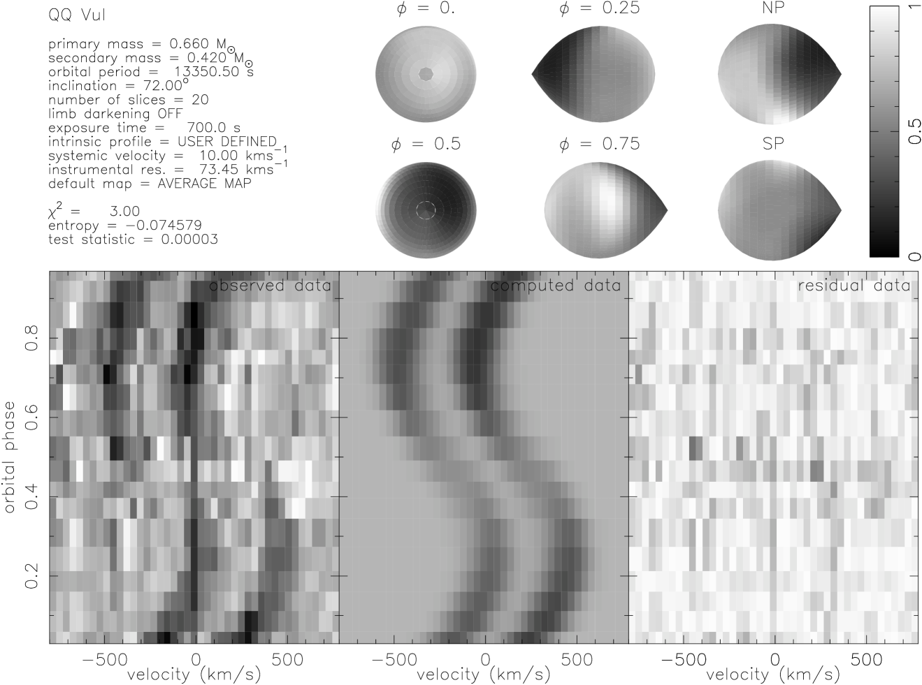
Figure 6: Roche tomogram of QQ Vul. Bright greyscales in the tomograms depict regions of enhanced Na I absorption. The greyscales are reversed in the trailed spectra. Note that the systemic velocity quoted in the upper-left of the panel does not take into account the systemic velocity of the spectral-type template star.

6 Results for IP Peg

6.1 The binary geometry of IP Peg

The optimum systemic velocity, as shown in Fig. 1, is –9 km s^-1. This is significantly different from the values of 56 $\pm$ 4 km s^-1 obtained by Martin, Jones & Smith (1987) and 31 $\pm$ 7 km s^-1 obtained by Martin et al. (1989). Fig. 1 also shows that we have been unable to determine the inclination of IP Peg. This is due to the small variations in the line strength over the orbital cycle, which provides our only constraint on the inclination before taking into consideration the eclipse width. The reconstructions do, however, yield a consistent result of 0.43 for the mass ratio of IP Peg (Fig. 2). This is in disagreement with $q$ = 0.55–0.63 and $q$ = 0.55–0.62 found by Martin et al. (1989) and Marsh (1988), but agrees with 0.35$<$q$<$0.49 (Wood & Crawford, 1986), $q$ = 0.39$\pm$0.04 (Catalán, 1999) and $q$ = 0.32$\pm$0.08 (Beekman et al., 2000). All the authors, except Beekman et al. (2000), made corrections for the effects of irradiation where appropriate.

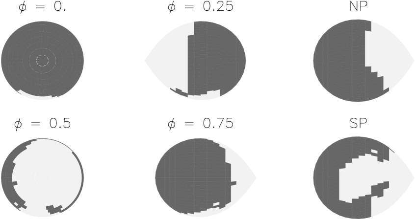
Figure 7: The significance map of QQ Vul, taking the comparison level to be the average intensity of the outer-hemisphere, avoiding both the irradiated regions and the bright area on the leading hemisphere. Bright greyscales indicate regions where the ‘true’ map ranks above 100 per cent of the ‘scatter’ maps. The significance of the region near the south pole (SP) is an artefact since this region is never observed.

Although we cannot determine the inclination using the surface maps alone, IP Peg is an eclipsing system, and its geometry is further constrained by the observed eclipse width, which is dependent upon the inclination and size of the secondary star’s Roche lobe. Fig. 3 shows the entropy landscape constructed by varying the inclination at each different mass pairing in order to match the eclipse width of $\Delta\phi$ = 0.0863 (Wood & Crawford, 1986). This results in optimum masses of $M_{1}$ = 1.18 M_⊙ and $M_{2}$ = 0.50 M_⊙ at an inclination of 82.3^∘. Altering the eclipse width to the other extreme of $\Delta\phi$ = 0.0918 given by Wood & Crawford (1986) changes this determination to $M_{1}$ = 1.16 M_⊙ and $M_{2}$ = 0.50 M_⊙ and the optimum inclination to 84.4^∘. Our best estimates are therefore $M_{1}$ = 1.16 – 1.18 M_⊙, $M_{2}$ = 0.50 M_⊙ and $i$ = 82^∘–85^∘.

Our secondary star mass determination appears to lie between the values of $M_{2}$ = 0.59–0.75 M_⊙ (Martin et al., 1989), $M_{2}$ = 0.55–0.73 M_⊙ (Marsh, 1988) and $M_{2}$ = 0.33${}^{+0.14}_{-0.05}$ M_⊙ (Beekman et al., 2000), $M_{2}$ = 0.33$\pm$0.07 M_⊙ (Catalán, 1999).

The primary mass is consistent with the values of $M_{1}$ = 1.05–1.25 M_⊙ determined by Martin et al. (1989), $M_{1}$ = 0.99–1.19 M_⊙ (Marsh, 1988) and $M_{1}$ = 1.05${}^{+0.14}_{-0.07}$ M_⊙ (Beekman et al., 2000), but slightly larger than $M_{1}$ = 0.85$\pm$0.09 M_⊙ determined by Catalán (1999).

6.2 The surface map of IP Peg

The Roche tomogram of IP Peg in the light of the Na I absorption doublet is shown in Fig. 8. The most noticeable feature is the weakened absorption flux deficit on the inner hemisphere of IP Peg, which can be attributed to irradiation. The effects of irradiation appear to be strongest, however, towards the leading hemisphere of the secondary star. We also see a bright patch of enhanced Na I absorption on the leading hemisphere similar to that seen in QQ Vul (Section 5.2).

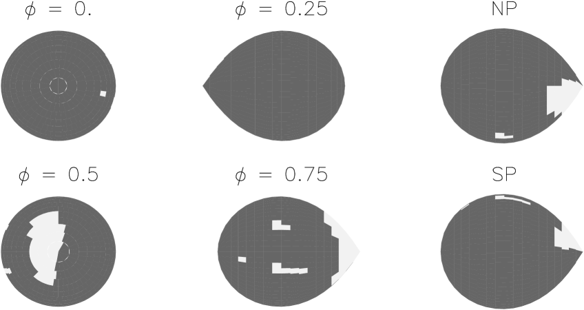
Figure 9: The significance map of IP Peg, taking the comparison level to be the average intensity of the outer-hemisphere avoiding the bright region on the leading hemisphere. Bright greyscales indicate regions where the ‘true’ map ranks above 100 per cent of the ‘scatter’ maps.

The significance map constructed taking the comparison level to be the average intensity of the outer hemisphere, avoiding the bright patch, is shown in Fig. 9. From this we can see that the bright patch is not significant, whereas the irradiated region on the leading hemisphere is.

In their radial velocity curve-fitting studies, Davey & Smith (1992) also found that the effects of irradiation were strongest on the leading hemisphere, and that regions of IP Peg appeared to be irradiated some distance onto the back half of the star. They found that this feature could not be explained by irradiation from the bright spot, as the illuminating source would have to originate from a direction about 45^∘ away from the line of centres and instead attributed this asymmetry to circulation currents (e.g. Martin & Davey 1995).

It is clear in Fig. 8 that we cannot identify any significant irradiation effects on the back half of the star and, as such, cannot provide any support for the evidence of circulation currents on IP Peg. It seems likely, instead, that the irradiation of the leading hemisphere can be explained by the bright spot, which is located on the correct side of the secondary star to cause this effect, and is a strong illuminating source (as seen in, for example, Szkody 1987).

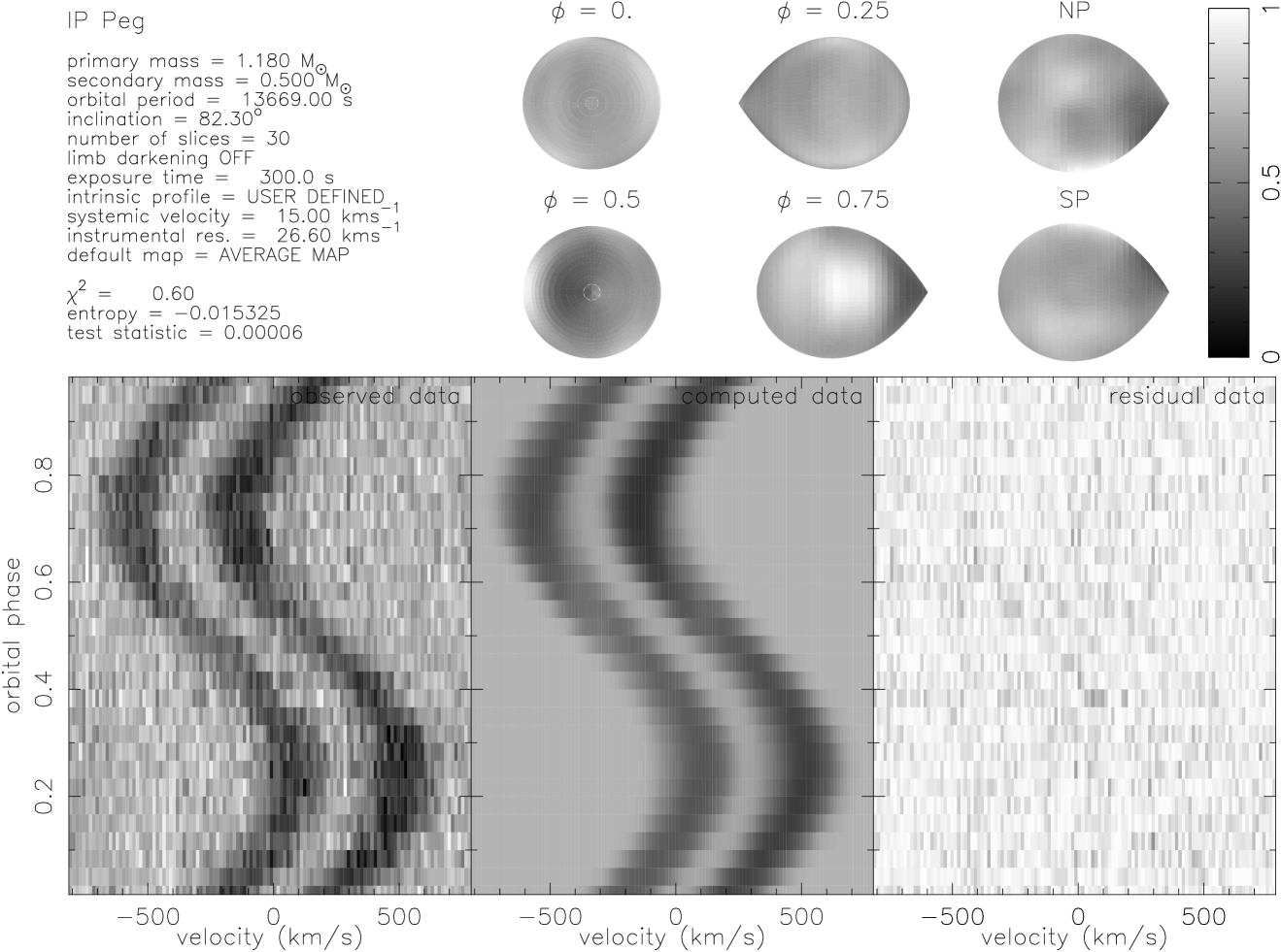
Figure 8: Roche tomogram of IP Peg. Bright greyscales in the tomograms depict regions of enhanced Na I absorption. The greyscales are reversed in the trailed spectra. Note that the systemic velocity quoted in the upper-left of the panel does not take into account the systemic velocity of the spectral-type template star.

Our Roche tomogram, however, bears little resemblance to the surface map that Davey & Smith (1992) computed from a model for a secondary star heated equally by the bright spot and the white dwarf (their Fig. 15), in that there does not appear to be any significant signs of irradiation on the trailing hemisphere. This suggests that irradiation from both the white dwarf and the bright spot is shielded from this region. An obvious way to block irradiation from the surface of the white dwarf is through shielding by the accretion disc. Irradiation from the bright spot may be blocked by the accretion stream, especially if much of the emission from the bright spot is located downstream from the impact point, as suggested in the eclipse maps of IP Peg by Bobinger et al. (1999). This would result in shielding of the trailing hemisphere, but still allow the bright spot to irradiate the leading hemisphere.

One further explanation for the features seen around the $L_{1}$ point is that they could be caused by the effects of an eclipse of the secondary star by the accretion disc. This would cause darker regions to appear in the Roche tomogram around the $L_{1}$ point and a reduction in the quality of the fit. Reconstructions carried out neglecting phases between 0.45–0.55 show no improvement in the quality of the fit, and there is negligible difference in the Roche tomograms. We are therefore confident that these features are not the result of an eclipse.

7 Results for HU Aqr

7.1 The binary geometry of HU Aqr

Fig. 1 shows the systemic velocity and inclination of HU Aqr as a function of entropy. We obtain a value of $\gamma$ = 7 km s^-1 and, although it is difficult to assign a value to the inclination, the reconstruction quality begins to decrease rapidly for inclinations less than 80^∘, and we therefore adopt a best estimate of $i\geq$ 80^∘.

Our estimate of the systemic velocity is compatible at the 2$\sigma$ level with $\gamma$ = 83 $\pm$ 44 km s^-1 derived by Glenn et al. (1994) who fitted a sinusoid to the narrow H$\alpha$ component thought to originate from the secondary star. Schwope et al. (1997) derived a systemic velocity of –7.8 $\pm$ 1.4 km s^-1 by fitting radial velocity curves to the same data used in this work. Although this result disagrees with the value obtained using Roche tomography, the sine-fitting method takes no account of any non-uniform intensity distribution present on the secondary star, whereas Roche tomography does. Since there is clearly an asymmetrical intensity distribution on the secondary star in HU Aqr (see Section 7.2) we believe that this is the cause of the difference between the two results.

In order to test the reliability of the sine-fitting method in determining the systemic velocity, we generated a model secondary star with the same binary geometry as we have found for HU Aqr in this work ($M_{1}$ = 0.61 M_⊙, $M_{2}$ = 0.15 M_⊙ and $i$ = 84.4^∘, see later) but with $\gamma$ = 0 km s^-1. The inner hemisphere of the model was then uniformly irradiated except for a totally dark shadow covering 40 per cent of the leading hemisphere. The outer hemisphere of the secondary star was also set to be totally dark. From this model, trailed spectra of infinite signal-to-noise were generated, assuming 100 equally spaced phase bins and 30 second exposure lengths.

By fitting radial-velocity curves to this fake data, we obtained a systemic velocity of –14 km s^-1. Fig. 10 shows the result of the radial-velocity curve fit (solid line) to the synthetic trailed spectrum, and the true motion of the centre-of-mass of the secondary star (dashed line) for comparison. The value of $\gamma$ = –14 km s^-1 is significantly different from the true value of $\gamma$ = 0 km s^-1 used in the model, and brings our systemic velocity of 7 km s^-1 into agreement with the value of –7.8 $\pm$ 1.4 km s^-1 obtained by Schwope et al. (1997). This shows that a knowledge of the intensity distribution across the secondary is required to accurately determine the systemic velocity (as also found by Schwope et al. 1997). This may have implications for the accurate determinations of $\gamma$’s used in CV age tests (e.g., van Paradijs, Augusteijn & Stehle 1996 and North et al. 2002).

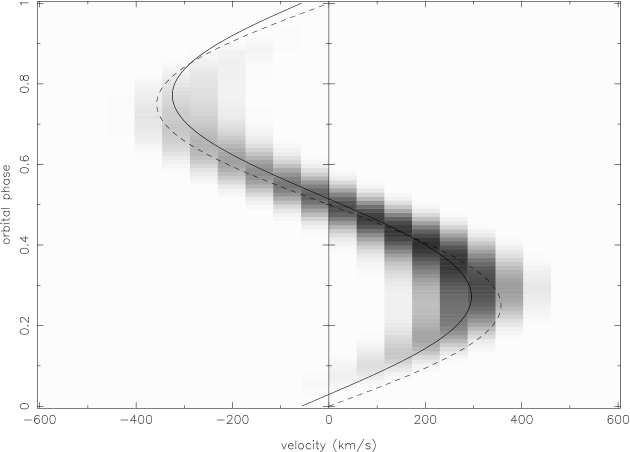
Figure 10: The synthetic trailed spectrum used to test the reliability of the sine-fitting method for the purposes of determining the systemic velocity. See the text for a description of the model used to generate the synthetic data (Section 7.1). The solid line corresponds to the radial-velocity curve fit and the dashed line corresponds to the true motion of the centre-of-mass of the secondary star. Note that the radial-velocity curve fit has also adjusted the zero point to $\phi$ = 0.02.

Since HU Aqr is an eclipsing system, its inclination has been reasonably constrained by previous studies, including estimates of $i$ = 80${}^{\circ}\pm$5^∘ (Glenn et al., 1994) obtained from fits to polarisation curves, and $i$ = 85.6^∘ (Schwope et al., 2001) from modelling the soft X-ray light-curves. Our determination of $i\geq$ 80^∘ does not provide any further constraint to those values already published.

Previous estimates of the mass ratio, however, are somewhat more uncertain and range from roughly 0.18 – 0.4 (e.g. Schwope et al. 1997, Hakala et al. 1993 and Heerlein, Horne & Schwope 1999). Fig. 2 shows the component masses and mass ratio obtained when reconstructions are carried out over different inclinations. This yields a mass ratio for HU Aqr of $q$ = 0.25, which is in excellent agreement with $q$ = 0.256 derived by Heerlein et al. (1999) assuming $i$ = 84^∘, and the value of $q$ = 0.25 that Schwope et al. (2001) found.

Fig. 3 shows the entropy landscape for HU Aqr which has been constructed by changing the inclination at each different mass pairing in order to match the eclipse width of $\Delta\phi$ = 0.0763 (Heerlein et al., 1999), as described for IP Peg in Section 6.1. This results in a best estimate of the component masses of $M_{1}$ = 0.61 M_⊙ and $M_{2}$ = 0.15 M_⊙. This agrees with the result of Schwope et al. (2001), who determined $M_{2}$ = 0.15 M_⊙ using the mass-radius relation of Caillault & Patterson (1990), and $M_{2}$ = 0.17 M_⊙ according to the relation by Neece (1984). Our derived masses, combined with the eclipse width, give our best estimate of the inclination as 84.4^∘.

7.2 The surface map of HU Aqr

The Roche tomogram of HU Aqr in the light of the He II 4686Å emission line is presented in Fig. 11. The two most prominent features in the Roche tomogram are the strong asymmetry between the inner and outer hemispheres of the secondary star and the weaker asymmetry between the leading and trailing hemispheres. The emission from the inner hemisphere is due to irradiation from the primary and the accretion regions, and the tomogram is compatible with 90 per cent of the emission arising from the inner hemisphere alone. (Note that the remainder of the emission that arises on the outer hemisphere is most likely due to the smearing effects of the default map).

The reality of the asymmetry between the leading and trailing hemispheres can be assessed from the left-most panel in Fig. 12, which shows a slice passing through the leading hemisphere (LH), north pole (NP), trailing hemisphere (TH) and south pole (SP) near the $L_{1}$ point of the secondary star. The triangular points represent the ‘true’ map values; 67 per cent of the bootstrapped ‘trial’ maps (measured relative to the mode of the distribution) lie within the solid line, and 100 per cent within the dotted line. It is clear from this that the asymmetry between the leading and trailing hemispheres is not due to statistical errors. This asymmetry was also found by Schwope et al. (1997) who attributed it to shielding by the accretion curtain.

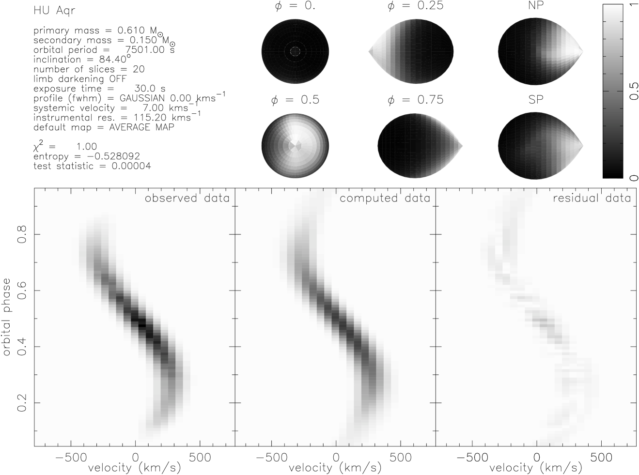
Figure 11: Roche tomogram of HU Aqr. Bright greyscales in the tomograms depict regions of enhanced He II $\lambda$4686Å emission. The greyscales are reversed in the trailed spectra.

Figure 12: The left-hand panel shows a vertical slice (see text for explanation) through HU Aqr near the $L_{1}$ point; the right-hand panel shows a vertical slice through HU Aqr closer to the terminator. The triangular points show the intensities found in the original fit. The lines show confidence limits derived from 200 bootstrapped reconstructions. The labels on the top axis denote the positions of pixels located on the leading hemisphere (LH), north pole (NP), trailing hemisphere (TH) and south pole (SP).

Closer examination of the tomogram reveals more subtle intensity variations across the secondary star. In particular there appears to be a region of more intense emission located towards the north pole but shifted slightly towards the leading hemisphere. The plot on the right hand-side of Fig. 12 shows a vertical slice cutting through the secondary star close to the polar regions but slightly towards the $L_{1}$ point. This again shows the shadow on the leading hemisphere (LH) as discussed earlier, but another feature of note is the drop in emission from the trailing hemisphere (TH) compared to the polar regions. This feature is not apparent near the $L_{1}$ point and only becomes significant for regions halfway between the centre-of-mass of the secondary and the $L_{1}$ point, disappearing again when the effects of irradiation are diminished near the terminator. This cannot be explained by shielding of the secondary star by the accretion curtain, since this would only block irradiation on the leading hemisphere.

HU Aqr does, however, have a strong stream component with as much as 40 per cent of the flux in the U band due to accretion stream emission (Hakala et al., 1993). Doppler maps by Schwope et al. (1997) also show that the accretion stream is a dominant emission-line feature. Presumably the accretion stream can also irradiate the secondary star and, since the stream is deflected in the direction of the orbital motion, the stream will be invisible to regions of the secondary star on the trailing hemisphere away from the $L_{1}$ point. This obscuration of the accretion stream by the secondary star itself may explain the observed shadow on the trailing hemisphere.

This feature could also be explained if systematic errors were able to produce a greater line flux in the centres of the lines, corresponding to artificially brighter polar regions in the Roche tomograms and giving the illusion of a shadow at lower latitudes. It was first thought that the assumption of a Gaussian profile for the emission from the secondary star could introduce such an artefact, since the actual profile from the secondary star is expected to be flatter, especially around quadrature. We found, however, that at low spectral resolutions the emission profile from the secondary is well approximated by a Gaussian. Artefacts could be generated if the emission from the various components of HU Aqr (e.g. from the secondary star and the accretion stream) are incorrectly disentangled, which is especially difficult at phases where the individual components are crossing each other. This situation is more difficult to assess and emphasises the importance of mapping lines that are known to originate solely from the secondary star.

8 Conclusions

The Roche tomograms show an asymmetric irradiation pattern on all 4 CVs. This can be explained if the accretion column/stream shields the leading hemisphere in AM Her, QQ Vul and HU Aqr. There is also evidence for a fainter shadow present on the trailing hemisphere of HU Aqr. We propose that the stream itself contributes significantly to the irradiation, and that the shadow on the trailing hemisphere occurs as these regions on the secondary star have no direct view of the majority of the stream. Further observations using absorption lines originating from the secondary star are needed to confirm this.

A different scenario occurs in IP Peg, where irradiation affects the leading hemisphere only. We suggest that the bright spot, which is on the correct side of the secondary star to cause such an irradiation pattern, may be the principal illuminating source in this system. Although we still expect irradiation of the trailing hemisphere by the white dwarf (as seen in the magnetic CVs), there is no evidence for this in the tomogram. It may be the case that the accretion disc in IP Peg is shielding the secondary star from irradiation by the white dwarf. Unlike Davey & Smith (1992), we find no evidence for irradiation extending onto the back half of the star, and hence cannot support their idea that circulation currents operate in IP Peg.

We have used the entropy landscape technique to derive the system parameters. Although we cannot reliably constrain the inclination, and therefore the masses, in the non-eclipsing CVs, the technique does provide a consistent result for the mass ratio that is independent of the inclination. For the two eclipsing CVs (IP Peg and HU Aqr), we believe that the masses derived in this work are the most accurate to date. In addition, it is found that measurements of the systemic velocity using circular orbit fits to the radial-velocity variations are unreliable, and are dependent upon the intensity distribution across the secondary star. We might therefore expect such measurements to be both line and time-dependent. Since the intensity distribution across the secondary star is known in Roche tomography, systemic velocity measurements using this technique should prove far more accurate.

References

- Beekman et al. (2000) Beekman G., Somers M., Naylor T., Hellier C., 2000, MNRAS, 318, 9
- Belle et al. (2000) Belle K. E., Howell S. B., Mills A., 2000, PASP, 112, 343
- Bleach et al. (2000) Bleach J. N., Wood J. H., Catalán M. S., Welsh W. F., Robinson E. L., Skidmore W., 2000, MNRAS, 312, 70
- Bobinger et al. (1999) Bobinger A., Barwig H., Fiedler H., Mantel K.-H., Šimić D., Wolf S., 1999, A&A, 348, 145
- Brainerd & Lamb (1985) Brainerd J. J., Lamb D. Q., 1985, in Lamb D. Q., Patterson J., eds, Proceedings of the 7th North American Workshop on Cataclysmic Variables and Low Mass X-Ray Binaries Reidel, Dordrecht, p. 247
- Brett & Smith (1993) Brett J. M., Smith R. C., 1993, MNRAS, 264, 641
- Caillault & Patterson (1990) Caillault J.-P., Patterson J., 1990, AJ, 100, 825
- Catalán (1999) Catalán M. S., 1999, private communication
- Catalán et al. (1999) Catalán M. S., Schwope A. D., Smith R. C., 1999, MNRAS, 310, 123
- Cropper (1988) Cropper M., 1988, MNRAS, 231, 597
- Cropper et al. (1998) Cropper M., Ramsay G., Wu K., 1998, MNRAS, 293, 222
- Davey & Smith (1992) Davey S., Smith R. C., 1992, MNRAS, 257, 476
- Davey & Smith (1996) Davey S., Smith R. C., 1996, MNRAS, 280, 481
- Dhillon & Watson (2001) Dhillon V. S., Watson C. A., 2001, in Boffin H., Steeghs D., eds, Astrotomography: Indirect Imaging Methods in Observational Astronomy Springer-Verlag Lecture Notes in Physics, Berlin, p. 94
- Donati et al. (1992) Donati J.-F., Brown S. F., Semel M., Rees D. E., Dempsey R. C., Matthews J. M., Henry G. W., Hall D. S., 1992, A&A, 265, 682
- Gänsicke et al. (1998) Gänsicke B. T., Hoard D. W., Beuermann K., Sion E. M., Szkody P., 1998, A&A, 338, 933
- Glenn et al. (1994) Glenn J., Howell S. B., Schmidt G. D., Liebert J., Grauer A. D., Wagner R. M., 1994, ApJ, 424, 967
- Gliese (1969) Gliese W., 1969, Vëroff. Astr. Rechen-Inst. Heidelberg., No. 22
- Greeley et al. (1999) Greeley B. W., Blair W. P., Long K. S., Raymond J. C., 1999, ApJ, 513, 491
- Hakala et al. (1993) Hakala P. J., Watson M. G., Vilhu O., Hassall B. J. M., Kellett B. J., Mason K. O., Piirola V., 1993, MNRAS, 263, 61
- Heerlein et al. (1999) Heerlein C., Horne K., Schwope A. D., 1999, MNRAS, 304, 145
- Horne (1986) Horne K., 1986, pasp, 98, 609
- Marsh (1988) Marsh T. R., 1988, MNRAS, 231, 1117
- Martin et al. (1989) Martin J. S., Friend M. T., Smith R. C., Jones D. H. P., 1989, MNRAS, 240, 519
- Martin et al. (1987) Martin J. S., Jones D. H. P., Smith R. C., 1987, MNRAS, 224, 1031
- Martin & Davey (1995) Martin T. J., Davey S. C., 1995, MNRAS, 275, 31
- Mouchet (1993) Mouchet M., 1993, in Barstow M., ed., White Dwarfs: Advances in Observation and Theory Kluwer, Dordrecht, p. 411
- Mukai & Charles (1987) Mukai K., Charles P. A., 1987, MNRAS, 226, 209
- Neece (1984) Neece G. D., 1984, ApJ, 277, 738
- North et al. (2002) North R. C., Marsh T. R., Kolb U., Dhillon V. S., Moran C. K. J., 2002, MNRAS, 337, 1215
- Nousek et al. (1984) Nousek J. A., Takalo L. O., Schmidt G. D., Tapia S., Hill G. J., Bond H. F., Grauer A. D., Stern R. A., Agrawal P. C., 1984, AJ, 277, 682
- Rutten & Dhillon (1994) Rutten R. G. M., Dhillon V. S., 1994, A&A, 288, 773
- Schwope et al. (2000) Schwope A. D., Catalań M. S., Beuermann K., Metzner A., Smith R. C., Steeghs D., 2000, MNRAS, 313, 533
- Schwope et al. (1997) Schwope A. D., Mantel K.-H., Horne K. D., 1997, A&A, 319, 894
- Schwope et al. (2001) Schwope A. D., Schwarz R., Sirk M., Howell S. B., 2001, A&A, 375, 419
- Shahbaz (1998) Shahbaz T., 1998, MNRAS, 298, 153
- Skilling & Bryan (1984) Skilling J., Bryan R. K., 1984, MNRAS, 211, 111
- Smith & Dhillon (1998) Smith D. A., Dhillon V. S., 1998, MNRAS, 301, 767
- Smith (1995) Smith R. C., 1995, in Buckley D. A. H., Warner B., eds, Cape Workshop on Magnetic CVs ASP Conference Series, San Francisco, p. 417
- Southwell et al. (1995) Southwell K. A., Still M. D., Smith R. C., Martin J. S., 1995, A&A, 302, 90
- Szkody (1987) Szkody P., 1987, AJ, 94, 1055
- van Paradijs et al. (1996) van Paradijs J., Augusteijn T., Stehle R., 1996, A&A, 312, 93
- Vogt & Penrod (1983) Vogt S. S., Penrod G. D., 1983, PASP, 95, 565
- Wade & Horne (1988) Wade R. A., Horne K., 1988, ApJ, 324, 411
- Watson & Dhillon (2001) Watson C. A., Dhillon V. S., 2001, MNRAS, 326, 67
- Wickramasinghe et al. (1991) Wickramasinghe D. T., Bailey J., Meggitt S. M. A., Ferrario L., Hough J., Tuohy I. R., 1991, MNRAS, 251, 28
- Wilson (1953) Wilson R. E., 1953, Carnegie Institute Washington D.C. Publication
- Wolf et al. (1993) Wolf S., Mantel K. H., Horne K., Barwig H., Schoembs R., Baerbantner O., 1993, A&A, 273, 160
- Wood & Crawford (1986) Wood J. H., Crawford C. S., 1986, MNRAS, 222, 645
- Wu et al. (1995) Wu K., Chanmugam G., Shaviv G., 1995, ApJ, 455, 260
- Young et al. (1981) Young P., Schneider D. P., Shectman S. A., 1981, ApJ, 245, 1043