Star forming rates between $z=0.25$ and $z=1.2$ from the CADIS emission line survey.

The emission line survey within the Calar Alto Deep Imaging Survey (CADIS) detects emission line galaxies by a scan with an imaging Fabry-Perot interferometer. It covers 5 fields of $>100\,\squareforqed\arcmin$ each in three wavelengths windows centered on $\lambda\simeq 700$, 820, and 920 nm, and reaches to a typical limiting line flux of $3\times 10^{-20}$ W m^-2. This is the deepest emission line survey covering a field of several 100 $\squareforqed\arcmin$. Galaxies between $z=0.25$ and $z=1.4$ are detected by prominent emission lines (from H$\alpha$ to [O ii]372.7) falling into the FP scans. Additional observations with a dozen medium band filters allow to establish the line identification and thus the redshift of the galaxies to better than $\sigma_{\rm z}=0.001$. On the basis of a total of more than 400 emission line galaxies detected in H$\alpha$ (92 galaxies), [O iii]500.7 (124 galaxies), or [O ii]372.7 (222 galaxies) we measure the instantaneous star formation rate (SFR) in the range $0.24<z<1.21$. With this purely emission line selected sample we are able to reach much fainter emission line galaxies than previous, continuum-selected samples. Thus completeness corrections are much less important. Although the relative [O iii] emission line strength depends on excitation and metallicity and shows strong variation, the mean line ratios yield SFR[O iii] values consistent with the SFR evolution. Our results substantiates the indications from previous studies (based on small galaxy samples) that the SFR decreases by a factor of $\sim 20$ between $z=1.2$ and today. In fact, for a $\Omega_{\rm m}=0.3,\Omega_{\lambda}=0.7$ cosmology, we find an exponential decline $\dot{\rho}_{\rm SFR}\propto\exp(-t_{\rm lookback}/2.6$ Gyr). This decrease of the SFR with time follows an exponential law which is compatible with the decreasing galaxy merger rate as expected from model calculations. The inferred SF density is in perfect agreement with that deduced from the FIR emission of optically selected galaxies which is explained by a large overlap between both populations. We show that self-consistent extinction corrections of both our emission lines and the UV continua lead to consistent results for the SF density.

1 Introduction

A number of studies of the star forming rate (SFR) were performed at different redshift regimes between the present epoch (Gallego et al. 1995) over intermediate redshifts (Tresse & Maddox 1998; Sullivan et al. (2000, 2001); Lilly et al. 1996; Cowie et al. 1997; Connolly et al. 1997) up to redshifts $\sim 3$ (Madau et al. 1996; Pettini et al. 1998). Their results suggest, that the SFR has declined from a maximum plateau at $z\sim 1.5$ to an one order of magnitude lower value in the present time.

The most direct way to determine the SFR is to observe the luminosity density of the H$\alpha$ line, which is little affected by extinction, excitation, and metallicity, and for which Kennicutt (1983, 1992) has derived a well established calibration relation. For redshifts higher than 0.4, however, it is necessary to use emission lines other than H$\alpha$, the luminosity of which are not so clearly related to SFR (Cowie et al. 1997; Hogg et al. 1998; Rosa-Gonzalez et al. 2002), or to observe in the near infrared (Yan et al. 1999; Teplitz et al. 2000; Pettini et al. 2001). Observations in the far infrared generally led to higher rates (Rowan-Robinson et al. 1997; Hughes et al. 1998; Flores et al. 1999)

As shown by Lilly et al. (1996), the star formation can also be derived from the UV luminosity of galaxies. Here however, the conversion to the SFR is severely affected by internal extinction, and for several years there was a huge gap between UV determined rates and the rates derived by other observational methods, since the proper extinction correction was not known. Recent studies of the reddening in starburst galaxies (Calzetti et al. 1994, Jansen et al. 2001) have succeeded to close this gap by providing more reliable correction factors.

Studies to relate the Balmer line luminosities to those of other emission lines and to the UV have been performed by Bell & Kennicutt (2001) for the local universe, by Sullivan et al. (2000) for $z\sim 0.15$, by Glazebrook et al. (1999) for $z=0.9$, and recently by Rosa-Gonzalez et al. (2002).

In the study presented here a new observational technique is applied to derive star forming rates and their evolution in the redshift range 0.25 to 1.2: The emission line luminosities for medium redshift galaxies are measured photometrically on deep narrow band images.

The search and classification of emission line galaxies is based on both the multi-color and the Fabry-Perot observations of the Calar Alto Deep Imaging Survey (CADIS). While in previous determinations of the star forming rates from emission line luminosity densities the object samples were selected via broad band magnitudes, in the present study it is based on the strength of the emission lines directly. Since spectrophotometric observations reach fainter limiting magnitudes than spectroscopic ones, the CADIS survey can reach galaxies with very low continuum brightnesses down to the extreme case of galaxies which are only detectable by their emission lines. In addition, the multi-color survey also provides UV luminosities, which allow within one and the same data base the comparison of the emission line luminosity densities with those in the UV.

The strategy of this deep imaging survey is to perform narrow band observations of relatively large fields in order to detect emission line objects down to very low line fluxes. In addition 15 broad and medium images are observed which are used to detect secondary emission lines and to derive spectral energy distributions for all detectable objects. These data are used to determine the spectral types and redshifts for a large number of galaxies by means of a multi-color classification routine.

Throughout this paper we use $\Omega_{\rm m}=0.3$, $\Omega_{\Lambda}=0.7$; $H_{\rm 0}=70$ km sec^-1 Mpc^-1 if not parameterized by $h$.

2 Observations and data handling

2.1 Observations

The observational principle of the CADIS survey is described in Meisenheimer et al. (2002). In the present paper we will only address in detail the observational and reduction procedures relevant to the study of emission line galaxies.

The observations are performed on a number of fields distributed over the sky selected at areas of minimum IRAS 100 $\mu$m emission (low galactic extinction) and free of bright stars.

In order to detect emission line objects, narrow band observations were done in three wavelength windows, which are relatively free from OH night-sky emission. In each of these windows observations are performed with a scanning Fabry-Perot interferometer (FPI) at 8 or 9 equally spaced wavelength steps, thus providing a spectral line scan (henceforth called FP scan). The three wavelength windows are specified by A, B, and C, and are located at:

window   FP-A :     $\lambda=702\pm 6$ nm,
window   FP-B :     $\lambda=820^{+4.5}_{-6}$ nm,
window   FP-C :     $\lambda=918\pm 8$ nm.

For selecting the correct interference order of the FPI, pre-filters with FWHMs of $\sim 20$ nm are used.

The FP observations in the B window were carried out with the CAFOS focal reducer at the 2.2 m telescope on Calar Alto, Spain; those in the A and C windows were carried out with the MOSCA focal reducer installed at the 3.5 m telescope. Both focal reducers are equipped with Fabry-Perot (Queensgate) etalons in the parallel beam, with free apertures of 50 and 70 mm, and with air gaps of $\sim$8 $\mu$m. By choosing the appropriate interference order, the spectral resolving power for both etalons was set, to $\sim$750 km s^-1. The actual spectral resolutions used were 1.8, 2.0, and 2.4 nm. Exposures were also done with the pre-filters alone in order to measure the continuum level underneath the emission lines found in the FP scans. At the 2.2 m telescope a flux limit of $F_{\rm lim}=3\times 10^{-20}$ W m^-2 was achieved after 3 hours of integration, sufficient to detect line emission of a galaxy with a star forming rate of $\sim$1.0 M_⊙ y^-1 at redshift z=1.2.

Table 1: Emission lines and corresponding (veto) filters for measuring their fluxes; filter specifications are noted in terms of central wavelength / full width at half maximum, both given in nm.

redshift	FP	FP	Filter used to observe
bin	line	Window	H$\alpha$	[OIII]	H$\beta$	H$\gamma$	[OII]
0.25	H$\alpha$	820 nm	FP-B	628/17	611/16	535/14	465/9
0.40	H$\alpha$	918 nm	FP-C	702/18	-	611/16	522/16
				+ FP-A
0.40	[OIII]	702 nm	909/30	FP-A	-	611/16	522/16
			+ FP-C
0.64	[OIII]	820 nm	-	FP-B	-	-	611/16
0.88	[OII]	702 nm	-	-	-	815/25	FP-A
1.20	[OII]	820 nm	-	-	-	-	FP-B

Since this observational method bears no color selection effect a priori, one expects to find also emission line galaxies with very faint continua, such as distant H ii galaxies and primeval galaxies at high redshift, detectable only in the light of their Lyman-$\alpha$ lines.

In order to decide which emission line was detected in the FP scan, we placed for each FPI band a set of medium band filters at wavelengths where secondary prominent lines would show up (Fig. 1). Since these filters allow to exclude certain line classifications - e.g., the presence of a line in any of these filters excludes that the line detected in the FP scan is [O ii] or Ly$\alpha$ -, they are named veto filters. These veto filters (see Table 1) are included in a the set of 15 medium and broad band filters, which range from 400 to 2200 nm in wavelength and provide additional information about the spectral energy distribution (SED) of the line emitter and its spectral type. Table 1 lists for the redshift bins discussed in the present paper, the filters where the secondary lines are expected.

2.2 Data base

The present study is based on the data sets from four fields (size $\sim 10\times 10$ arcmin) of the CADIS emission line survey which are completely reduced up to now, as listed in Table 2. In these fields we selected the emission line galaxies detected in the light of their prominent emission lines H$\alpha$, [O iii]$\lambda 500.7$, or [O ii].

For the window B around 820 nm, the data of the 01h, 09h, and 16h fields were used to derive luminosity functions and star forming rates at redshifts of $z=0.25$ (H$\alpha$ line), 0.64 ([O iii] line), and 1.2 ([O ii] line). For the window A, around 702 nm, the data of the 09h, 16h, and 23h fields were used. Here the redshifts studied are $z=0.40$ ([O iii] line), and $z=0.88$ ([O ii] line). The H$\alpha$ galaxies appearing at redshift 0.08 are too rare to provide a useful database. The data of window C were only used for consistency checks, but not for deriving luminosity functions and star forming rates, since the classification for this window is not yet fully understood.

Table 2: Fields observed with CADIS used in the present paper.

Field	FP	Center	coord.	Area
name	window	$\alpha$(2000)	$\delta$(2000)	arcmin2
01h	B	01h47m33.3s	02 19 55”	103
09h	A, B	09h13m47.5s	46 14 20”	100
16h	A, B	16h24m32.3s	55 44 32”	106
23h	A	23h15m46.9s	11 27 00”	98

The number of galaxies found per field and redshift interval, with emission line fluxes above our detection limit is of order of 30, providing emission line galaxy samples large enough for statistical studies (see also Table 3).

The wavelengths can be set with the FP etalon within an accuracy of $\pm 0.2$ nm. The wavelength calibration was done several times during the night using the calibration lamp lines Rb 794.5 nm and Ne 692.95 nm, and was stable within 0.15 nm during the observations. This is roughly one order of magnitude less than the width of the instrumental profile of $\sim 2.0$ nm, which was adjusted by selecting the appropriate interference order of the FPI. Towards the edges of the fields, the transmitted wavelengths declined by 0.5 nm, due to the increasing angle of incidence in the FP etalon. In combination with the dithering used for the observations, this leads to an additional wavelength uncertainty of $\pm 0.1$ nm in the edges of the frames. Including the error of the line fit (see Sect. 2.5), the total uncertainty for a medium strong line thus arises to about $\pm 0.4$ nm in $\lambda$, or about $\pm 0.0008$ in redshift. A comparison of the redshift values for objects with $z\sim 0.40$, which can be seen in both the window A (by their [O iii] line) as well as in window C (by H$\alpha$) yields the same value for the redshift uncertainty.

2.3 Data reduction

The data reduction includes subtraction of bias, flatfielding, and removal of cosmics and detector defects by overlaying dithered images and replacing the bad pixels by the kappa-sigma-clipped mean of pixel values in the other images.

Special care has to be taken for the flatfielding, since internal reflections between the focal reducer optics and the Fabry-Perot etalon can give rise to straylight contributions in the central area of the flatfields, thus leading to a incorrect flux calibration of the FP data. In order to overcome this problem, flat field exposures are taken through a regularly spaced multi-hole mask, allowing to measure the instrument transmission without noticeable straylight contribution.

After overlaying all images to the same world coordinate system, the images for each wavelength setting and filter are then added up. For each of these sum frames the object search engine SExtractor (Bertin & Arnouts, 1996) is applied, with thresholds adjusted to their seeing and exposure depth. The object positions are corrected for the distortion of the camera optics, and the object lists are merged to a MASTER table with averaged positions. For merging all objects are considered to be identical which fall into a common error circle of 1″ radius.

The morphology parameters of an object are determined on the sum frame where the object shows the highest S/N ratio, using the photometry package MPIAPHOT (Meisenheimer & Röser, 1993). The photometry is performed on each individual frame, by integrating the photons at the centroid object positions, with a Gaussian weight distribution, the width of which is determined such that the convolution of the seeing PSF with the weight function results in a common PSF for all frames. The obtained flux is then calibrated by tertiary spectroscopic standard stars established in each CADIS field. Finally, the single frame flux values are S/N-weight averaged with errors derived from the counting statistics. Since the photometry weight function is normalized to give correct fluxes for stellar objects, the fluxes of extended objects are underestimated and need a correction according to their morphological parameters.

2.4 Selection of emission line galaxy candidates

The pre-selection of emission line galaxies is based on the fluxes in the FP images and in the pre-filter image. Candidates have to fulfill two criteria: (1) For at least one FP wavelength, the signal has to be larger than the upper limit of the noise distribution, typically located near 5$\sigma$. (2) The signal-to-noise ratio of the line feature in the FP scans above the pre-filter flux is higher than  2.5, equivalent to about $2\times 10^{-20}$ W m^-2 (here we choose a very low threshold in order to be complete; a much stricter selection is possible on the basis of the line fits described below). This pre-selection yields a few hundred of emission line galaxy candidates per field and wavelength window.

Due to reflections within the Fabry-Perot etalons employed in CADIS, bright objects, mostly stars, are accompanied by features about 6 magnitudes fainter than the father object, and appear at a fixed offset position (41″) away from it. Since in the pre-filter images no object should be seen at the same positions, these ghosts can be easily sorted out and rejected from the candidates list.

Another type of ghosts on the single FP frames is produced by reflections of bright objects in between FP etalon and pre-filter. These ghosts appear symmetrically to the optical axes and, due to dithering, they show up at different positions in every frame. Thus these are easily identifiable and already strongly suppressed by the correction for cosmic rays in the standard data reduction.

Spurious objects were found to occur in the wings of bright objects, due to variations in the extended wings of the point spread function. A scatter of the flux measured in the Fabry-Perot images at the position of a spurious object can pretend an emission line. In order to find and reject these artifacts, all candidates with a bright neighbour were flagged. Based on eye inspection, a simple criterion was derived, which separates real objects from artifacts rather successfully: If

$m_{\rm R}({\rm next\,bright\,object})+dist({\rm arcsec})<m_{\rm crit}$,

with $m_{\rm crit}=24.0$, the feature is considered as an artefact and removed from the list of candidates. It was verified that this procedure does not lead to a loss of any “good” objects.

2.5 Analysis of emission line objects

After pre-selection, the emission line galaxy candidates are classified, by analysing their emission line features in the FP scans as well as their SEDs, determined by the multi-filter observations. For the classification, three criteria are used: the shape of the emission line observed with the FPI, the emission line spectrum, derived from medium band veto filters placed at wavelength where prominent secondary lines are expected, and the continuum SED.

This analysis and classification procedure is performed in five steps, which are described in the following in detail.

(1) Line Fit:

First step is the analysis of the photometric FP data by line fitting. The width of the line profiles are fixed to the width of the instrumental profile (1.8, 2.0, and 2.4 nm for the windows A, B, and C respectively) for the particular wavelength window.

Line fluxes were derived from the areas under the fitted line curves. For the fit, a modified Gaussian function was chosen of the form

$f(\lambda)=f_{\rm 0}\times exp\big{\{}-1.96|(\lambda-\lambda_{\rm 0}/\Delta\lambda|^{1.5}\big{\}}$,

where $\Delta\lambda$ is the instrumental resolution (FWHM). This function has a more pronounced peak and broader wings than the normal Gaussian profile, and is rather close to the shape of the instrumental profile of the FP etalon. The area under this line profile is $A=1.12f_{\rm 0}\times\Delta\lambda$. Accounting for the fact, that the wings of the real FP profile are somewhat broader than in the above function, we use $A=1.25f_{\rm 0}\times\Delta\lambda$. This factor was verified by a comparison of the fluxes of the [O iii] lines from $z\sim 0.4$ galaxies as determined in the FP scans (window A), with those determined from the excess flux in the medium band filter located at $\lambda=700$ nm above the continuum.

Since the detected line can be any emission line occurring in the observed wavelength window at the appropriate redshift (e.g., H$\alpha$ at 0.25, [O iii] at 0.64, etc., for the B window at 820 nm), the classification routine has to investigate the solutions for all bright emission lines. Thus, we consider a total of eight possible line identifications in our fitting procedure: [S ii] 673, H$\alpha$, [O iii] 501 and 496 nm, H$\beta$, H$\gamma$, [O ii], and Lyman-$\alpha$. The number of galaxies expected to be seen in other lines is negligible (see Sect. 3.3) and does not justify to include them into this list. The H$\alpha$ line fit includes the [N ii] doublet. With the the spectral instrumental resolution of $\sim 2.0$ nm it is possible to separate the [N ii] 658.3 line in about 50% of the cases successfully from the H$\alpha$ line with [N ii]658.3/H$\alpha$ line flux ratios in between 0.1 and 0.5. This is generally the case for $S/N(H\alpha)>4.4$. For the ten strongest H$\alpha$ emitter the ratio is [N ii]/H$\alpha=0.21\pm 0.05$. The maximum line flux ratio [N ii]658.3/H$\alpha$ is limited to 0.5 in the fit.

In order to make use of the pre-filter fluxes, the line flux estimated from this line fit is subtracted from the pre-filter flux allowing for the filter transmission at the specific wavelength of the line. The line corrected pre-filter flux - and its error - is included as an additional continuum data point for an improved line fit. Examples for fits to different lines are shown in the right panels of Fig. 1, where the observed pre-filter fluxes are marked as solid bars with their errors, and the corrected pre-filter fluxes as dashed lines. Both values are also marked in the SED plots in the left panels.

Figure 1: Emission line fits (right panels), and smoothed continuum fits (left panels) for a $R=22.9$ mag galaxy at redshift 0.250 (top), a $R=23.1$ mag galaxy at $z=0.638$ (second row), and a $R=23.4$ mag galaxy at $z=1.192$ (third row). In the bottom panel, a $R=23.3$ mag galaxy at $z=0.688$ is shown; since there is no filter placed at 840 nm, the strength of the [O iii] lines is unknown for this case. The numbers in the lower right edges of the right panels specify the signal-to-noise ratios for the line fits. Filled circles represent observed data, empty squares the emission-line corrected pre-filter fluxes.

(2) Continuum SED fit:

In the next step, for every of the eight redshifts determined above, template spectra published by Kinney et al. (1996) were fitted to the SED derived from the multi-filter photometry. This is done by means of colors, similar to the multi-color classification procedure described in Wolf et al. (2001), yielding a most probable template spectrum. In order to achieve better fits to the data, we allow for an extra reddening correction of the template spectra up to $E_{\rm B-V}$ of 0.3. The latter is important for distant samples which contain generally brighter and more massive galaxies with more reddening than the Kinney et al. templates (see sect. 3.5).

Since we want to determine the fluxes in the emission lines from the signal excesses in the veto filters above the continuum (see step 4), line free template spectra are needed. Thus, the Kinney-Calzetti template spectra were altered by cutting out the prominent emission lines. As a consequence, those filter data where secondary emission lines are expected, are not usable for the fit. Thus, the SED fit is purely based on the continuum part of the spectra.

For the template spectrum which fits best to the observed SED a reduced $\chi^{2}$ is derived.

(3) Improved line fit:

The fit to the continuum spectrum provides, for each of the eight possible line identifications, also a new continuum level at the wavelength of the FP window, which is marked in either of the line plots in Fig. 1 as a dotted horizontal line. The error bar is estimated from the quality of the continuum fit, and is comparable to that of the pre-filter flux. Ideally, this continuum flux level should agree with the corrected pre-filter flux (step 1). A high discrepancy between the two values indicates that either the SED fit is bad (due to incorrect line classification), or the line feature seen in the FP scan is awkward. This information is used to produce another $\chi^{2}$ contributor, calculated from the discrepancy and the intrinsic errors of the two flux levels.

Including the continuum level derived above, a new revised line fit is performed in the same way as in step 1. In this second iteration, however, bad line classifications become visible by large offsets between the continuum level given by the SED fit and the corrected pre-filter baseline, leading to a lower S/N ratio for the corresponding line fit. This also happens when the line feature in the FP data is in reality a fake detection due to a statistical fluctuation of the FP signals.

The new S/N value is later used as critical indicator for the reality of the line feature seen in the FP scan and whether the object will be accepted as an emission line galaxy.

(4) Line spectrum fit:

The continuum fit found this way serves as a baseline to determine the fluxes of the other (secondary) emission lines. For each of the eight possible line identifications, the fluxes for the secondary lines were derived from the difference between the flux measured in the ‘veto filters’ (the filters where other prominent lines would be expected) and the continuum level predicted from the template fit. For the calculation of the line strength, the excess flux was normalized by the transmission of the filter at the wavelength given by the redshift derived from the FP observation. In cases where the veto filter included more than one emission line which generally happens for the [O iii] 501/496 doublet, the line flux ratio was fixed to the canonical values. Fig. 1 shows such fits for several objects in the left panels. In all spectra, except for the [O ii] galaxy, a number of ‘secondary’ lines can be seen.

The thus determined line flux ratios are compared with a catalog of observed line ratios for about 500 nearby galaxies based on data from the literature, including a range of Seyfert galaxies to compact dwarfs, most notably from French (1980), McCall et al. (1985), Popescu & Hopp (2000), Veilleux & Osterbrock (1987), Vogel et al. (1993).

A $\chi^{2}$ is estimated in the following way: In the multidimensional space made up by all line ratio combination possible for the respective classification of the line observed in the FPI window, the mean distance of the considered galaxy to the three closest tabulated ratios was normalized by the error ellipse of the observed ratios. This method prevents a bias towards the most common line ratios, but allows also galaxies with extreme line ratios, as long as there are some objects with similar ratios tabulated. Again, a $\chi^{2}$ for the line ratios is estimated for each of the eight line cases.

(5) Finding the best solution:

To decide between the possible line identifications an overall reduced $\chi^{2}$ is derived, which is the mean of the four $\chi^{2}$ values, of the SED fit (see step 2), of the line fit (step 3), of the discrepancy of the baselines (step 3), and of the line ratios (step 4). This mean $\chi^{2}$ is then converted into an overall probability for the line classification according to   $P=exp(-\chi^{2}/2)$. The case with highest probability is then selected as the most probable classification.

Fig. 1 depicts three examples of SED and emission line fits for galaxies at redshifts 0.250, 0.638, and 1.192 with strong emission lines, together with an example for galaxy with a line signal near the S/N cutoff (see Sect. 3.1), which was classified as H$\beta$ at $z=0.686$, and verified spectroscopically to be at $z=0.687$. In the plot, the fluxes are given in units of  photons sec^-1 nm^-1 m^-2.

2.6 Comparison with spectroscopic observations

The decision, if an emission line galaxy candidate is considered as real or not is based on the S/N ratio of its line fit. To avoid contamination of the galaxy samples by fakes on the one hand and to be complete as possible on the other, an optimum S/N cutoff value has to be determined.

Spectroscopic follow-up observations were carried out for a number of emission line galaxy candidates with the MOSCA spectrometer at the 3.5m Calar Alto telescope, with LRIS at Keck, and with FORS1 at VLT. We use the results of these observations to compare them with the predictions from our emission line classification, and to find the optimum S/N for a reliable classification. This comparison is depicted in Fig. 2.

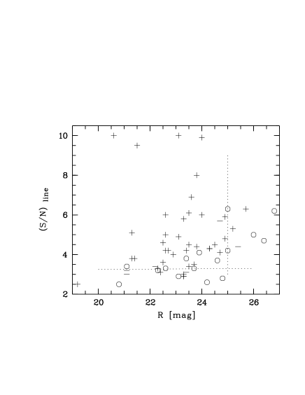
Figure 2: Correct and incorrect predicted line identifications for the spectroscopically observed galaxies, for varying $R$ magnitude and S/N ratio. + stands for correct, - for incorrect identification. A circle indicates, that no line could be verified at the predicted wavelength.

The diagram shows, that for a S/N cutoff at 3.3, and for $R<25$ mag (dotted lines), the probability for a correct classification is of the order of $80\%$. For fainter galaxies the continuum is obviously too weak and the signal too noisy to allow a reliable continuum fit. For a number of cases, the spectra showed a spatial offset between line emission and continuum object of up to 1″ (Maier et al. 2003). Considering that the slit generally centered on the continuum source is only 1.0″ wide, it seems possible that in those cases where an emission line detected in the FP scan could not be verified in the slit spectra (circles in Fig. 2), the slit actually missed the line emitting region. In those cases the photometric data derived from the imaging survey would tend to yield more reliable results than slit spectroscopy. A more careful analysis of the offsets between the continuum and line emission centroids resulting in excessive slit losses is currently in process.

3 Results

3.1 Final object selection

The emission line galaxy candidate samples, preselected according to the criteria described above, are now separated into the specific redshift ranges. The candidates are then subjected to a further selection procedure, where objects classified as quasars or stars in the multi-color classification are rejected. Both object types are also suspicious by very low overall probabilities $P$ of the line classification.

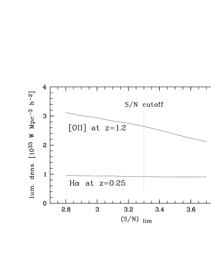
Figure 3: Line luminosity density plotted versus the chosen signal to noise limit for the [O ii] galaxies at $z=1.2$, and for the H$\alpha$ galaxies at $z=0.25$. Data are extinction corrected (see Sect. 3.5), but not completeness corrected.

Fig. 3 shows that the dependence of the resulting line luminosity density on the choice of the S/N limit for the emission line is not severe. As mentioned, a value of 3.3 seems to be appropriate. Lowering the cutoff line to $S/N=3.0$, which would include many artifacts and wrong identifications (see Fig. 2), the luminosity density in the case of the $z=1.2$ sample increases by only about 10%. For the galaxy sample at redshift 0.25, which is more complete at the faint end, the effect is even smaller. The choice of the cutoff mainly affects the completeness at the low luminosity end of the line luminosity function.

3.2 Sample statistics

The total numbers of objects in the fields studied, classified as H$\alpha$ galaxies, as [O iii]$\lambda$500.7 galaxies, and as [O ii] galaxies at the appropriate redshifts is listed in Table 3.

The number for galaxies seen in the other emission lines is too small for a useful statistical study. The expected number of galaxies detected by their [O iii] 495.9 line in the B window, for example, can be readily estimated from the statistics of the brighter [O iii] 500.7 line. Since the line intensity ratio of these lines is 3:1, the expected number is about that of the number of [O iii] 500.7 nm with a S/N greater than $3\times(S/N)_{\rm lim}=10.5$, which is only 7 galaxies. Therefore, in the following, [O iii] always stands for the brighter, the [O iii] 500.7 line. A similar argument leads to a total of 8 for the expected number of H$\beta$ line galaxies.

Table 3: Statistics for the emission line galaxies observed in the five redshift intervals (from 3 CADIS fields each).

Line	Window	Total	z range	S/N	N
		area		limit
H$\alpha$	B	309 $\squareforqed\arcmin$	0.238-0.252	3.3	92
[OIII]	A	300 $\squareforqed\arcmin$	0.390-0.411	3.3	44
[OIII]	B	309 $\squareforqed\arcmin$	0.626-0.646	3.3	80
[OII]	A	304 $\squareforqed\arcmin$	0.867-0.894	3.3	103
[OII]	B	309 $\squareforqed\arcmin$	1.175-1.210	3.3	119

The range of the equivalent widths at rest wavelength in which the emission line galaxies are detected, is plotted vs. M_B in Fig. 4 for the H$\alpha$ galaxies at redshift 0.25 and for the [O ii] galaxies at $z=1.2$. The absolute blue magnitude is calculated by interpolating between the flux densities from the medium and broad band filters left and right of $440(1+z)$ nm, and calibrating with Vega. The dotted lines indicate the sensitivity limit of the survey, at $F_{\rm line}=3\times 10^{-20}$ W m^-2. Note that our minimum detection limit $EW>0.2$ nm caused by photometric uncertainties, does not affect the sample statistics.

The distribution shown in this figure is consistent with the EW distribution of the CFRS sample (Hammer et al. 1997, Tresse & Maddox 1998). The mean line equivalent width of the Tresse & Maddox sample at $z\sim 0.2$ is $<$log $EW$(H$\alpha$+[NII])$>$=1.59 nm as compared to our mean value of 1.54. The considerably higher equivalent widths seen in nearby galaxy samples (Gallego et al. 1996, Ho et al. 1997, Terlevich et al. 1991) are not comparable, since their spectrograph slits cover only the central parts of these galaxies.

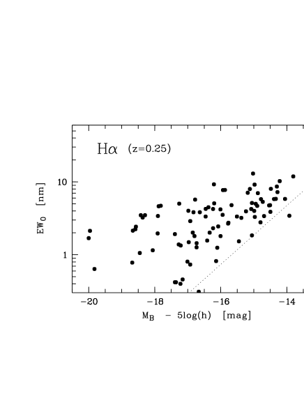
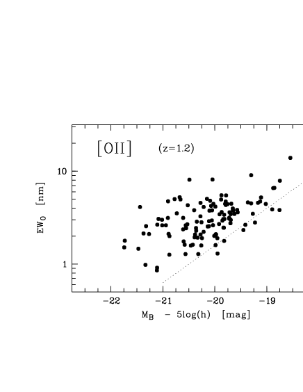
Figure 4: H$\alpha$ and [O ii]372.7 line equivalent widths at rest wavelength versus absolute blue magnitude; the dashed lines indicate the sensitivity limit of the emission line survey, at $F_{\rm line}=3\times 10^{-20}$ W m^-2.

For local galaxies Kennicutt (1992) established a mean ratio between [O ii] and H$\alpha$ eqivalent widths of 0.5. For galaxies identified in the B window by their H$\alpha$ line ($z=0.25$), we find a considerably higher ratio of  $\sim 0.9$. This finding agrees with the CFRS results by Hammer et al. (1997), who explain the difference by a lower metallicity and hotter star temperatures in their $z\sim 0.3$ sample, and/or by the lower luminosities as compared to the local galaxy sample of Kennicutt. The latter explanation would be consistent with the result of Gallagher et al. (1989), who find a higher EW[O ii]/EW(H$\alpha$) ratio for blue local galaxies as well.

3.3 Sample contamination

The contamination or incompleteness of our samples due to wrongly classified galaxies is of the order of $\pm$10% (see Fig. 2). One has, however, also to consider contamination by galaxy types not included in our ELG templates, such as galaxies seen in [O i] or in Mg ii in the FP spectra, and AGNs in general.

For discriminating these contaminants, we selected those emission line galaxies for which the CADIS multi-color classification (Wolf et al. 2001) yields a different line solution or indicates a quasar. After eye inspection of the spectra, two galaxies initally classified at $z=0.25$ were found to be at redshift 0.30 ([O i] at $\sim$820nm). Two possible quasars at redshift 1.2 and another two at 1.9 (Mg ii in window B) were recognized and removed from the [O ii] sample. Among the ELGs seen in the A window no QSO was found.

The line ratios measured by the CADIS emission line survey have relatively large error bars and do not allow to recognize Seyfert 2 galaxies, neither does the multi-color classification. Spectroscopy of AGNs in the Chandra deep fields indicate a surface density of 450 Sy2 galaxies per square degree at $R<24$ and $0.5<z<1$ (Szokoly et al., 2002), equivalent to only three Sy2 in our $z=1.2$ sample. At lower redshifts even fewer objects are expected.

LINERS are, among other, recognizeable by a high [Nii]/H$\alpha$ line flux ratio. The line fits for the 30 strongest line emitters in our $z=0.25$ sample yield two LINERS ($EW$[NII]/$EW$(H$\alpha$)$>$0.6). The contamination of the total H$\alpha$ luminosity by the [NII] fluxes from these two LINERs is about 2%. In the CFRS no low-excitation AGN was found (Hammer et al. 1997). Thus, we are confident that the LINER contamination is negligible in all our samples.

3.4 Luminosity functions

Fig. 5 shows the $M_{\rm B}$ luminosity functions for the H$\alpha$ and [O ii] galaxies observed in window B (average over 3 CADIS fields), and for the [O ii] galaxies observed in window A (average over 3 fields). The data points for the mean density are in agreement to the luminosity function obtained for the late type galaxies (later than Sa) in the respective redshift ranges, derived from the multi-color survey of CADIS (Fried et al. 2001). The Schechter functions overlaid in the figure are also adopted from Fried et al. and represent the sum of the two LFs for starburst galaxies and spirals in their paper.

This agreement suggests that in principle all late type galaxies at these redshifts are emission line galaxies with lines bright enough to be detected in the CADIS Fabry-Perot observations.

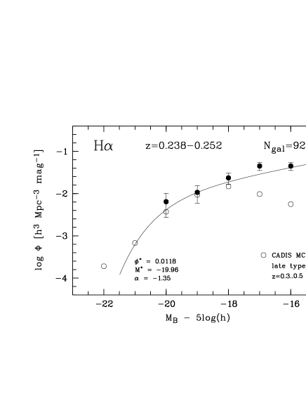
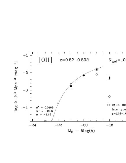
Figure 5: Luminosity functions for the emission line galaxies at $z=0.25$, 0.64, and 1.2 (filled circles). For comparison open circles trace the luminosity functions for late type galaxies according to the CADIS multi-color survey (Fried et al. 2001), together with the corresponding Schechter functions. Schechter parameters are given at the high luminosity ends of the curves.

3.5 Extinction correction

Since star forming regions are generally embedded in massive and dusty molecular clouds, extinction plays an important role in the determination of intrinsic line emission and can amount to more than a magnitude in the H$\alpha$ line.

The calibration factors used to convert the line luminosity densities into star formation rates are derived for unobscured line emission (Kennicutt 1983, 1992). So our line luminosities need to be corrected for extinction before deriving star formation rates. This correction is generally based on the H$\beta$/H$\alpha$ intensity ratio. In our data sample, the fluxes for the H$\beta$ line contain large relative errors, since the flux contained in the H$\beta$ line is in most cases not directly measurable, but only as blend with the [O iii] lines. Thus, a reddening correction for each individual galaxy is not possible.

There is, however, an observed trend in the sense that more luminous galaxies (disks) show higher reddening than less luminous ones, such as H ii galaxies, irregulars, BCDs (Gallego et al. 1997), which allows to perform a global correction based on the blue magnitude of each galaxy. This trend is clearly seen in the nearby galaxy sample used by Calzetti et al. (1994) to study the internal reddening. Their data suggest an increase of reddening according to

$E_{\rm B-V}=0.10\leavevmode\nobreak\ (M_{\rm B}+15.5)\leavevmode\nobreak\ \pm 0.15$.

with no difference between spirals and BCGs.

For a larger galaxy sample of nearby galaxies, Jansen et al. (2001) investigated the dependance of the [O ii]/H$\alpha$ emission-line ratio on other observables. They found that the large scatter of the observed ratio and its dependence on luminosity are greatly reduced when using reddening-corrected [O ii] fluxes. Their correlation between absolute magnitude and reddening, derived from the Balmer decrement after correction of the underlying stellar Balmer absorption, indicates a relation with a less steep slope:

$E_{\rm B-V}=0.064\leavevmode\nobreak\ (M_{\rm B}+14.8)\leavevmode\nobreak\ \pm 0.10$.

independent of the galaxy type. The large uncertainty, which is engendered by the large scatter of the data points and due to geometrical and excitation temperature effects, makes it impossible to predict the reddening for a particular galaxy. Since the present study, however, deals with global parameters instead of individual galaxies, it is appropriate to apply this relation for an averaged reddening correction. For faint galaxies ($M_{\rm B}>15.6$), we adopt a minimum reddening correction of $E_{\rm B-V}=0.05$ mag.

3.6 Luminosity functions for the emission line fluxes

The next step towards establishing global star forming rates is the determination of luminosity functions for the emission line fluxes. Fig. 6 shows these for the same three redshift intervals as in Fig. 5. In these diagrams, the sampling interval for the line luminosity was chosen as 0.4 dex, equivalent to 1 magnitude stepsize, in order to allow an easy comparison with the $M_{\rm B}$ luminosity functions.

In the $L_{\rm H\alpha}$ plot (top) the observed line luminosity data of Tresse & Maddox (1998) and by Cowie et al. (1997), after being converted to the cosmological parameters used in the present paper, are over plotted. In the $z=1.2$ panel, the Cowie et al. (1997) points are over plotted. Both agree satifactorily well with our data.

The extinction corrected luminosity functions are shown by filled symbols. For the case of the H$\alpha$ luminosity at $z=0.25$, the correction yields an increase of the total line luminosity by a factor of 1.6. For the $z=1.2$ sample the extinction correction amounts to a factor of about 4 in the total [O ii] line luminosity (see Table 4), due to both the higher blue luminosities of the galaxies and the shorter wavelength of the line.

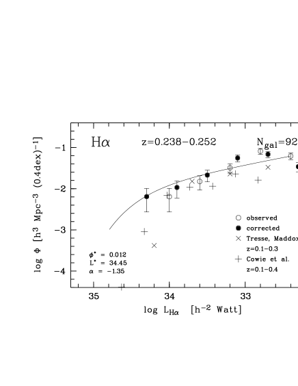
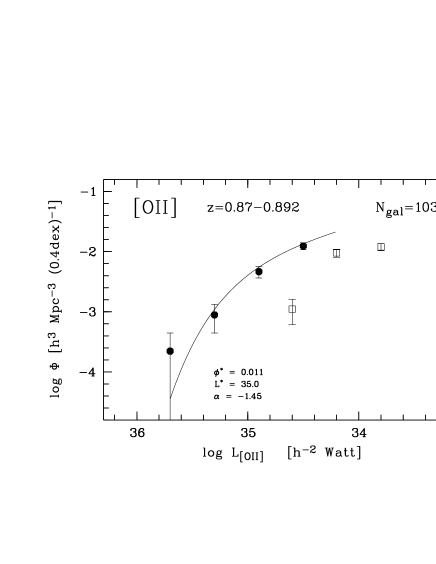
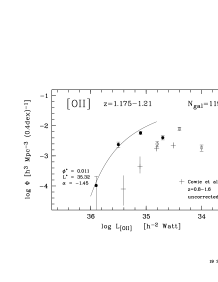
Figure 6: Luminosity functions for the observed H$\alpha$ line emission at redshift 0.25 (top), for the [O ii] line at redshift $z=0.88$, and for the [O ii] line at redshift $z=1.2$; open cirles are uncorrected, filled circles are extinction corrected values; for comparison, the observed (uncorrected) line luminosity function by Cowie et al. (1997) and by Tresse & Maddox (1998) are shown. The parameters for the Schechter functions plotted over the data have the same $\Phi$ and $\alpha$ as the M_B luminosity functions.

In several studies (Gallego et al. 1995, Tresse & Maddox 1998, and Yan et al. 1999) line luminosity functions were successfully described by Schechter functions, the parameters of which were derived by the V_max method. For small data samples, as it is the case in the present study, this procedure leads however to arbitrary results.

As can be seen in the plots, the H$\alpha$ luminosity density histogram (z=0.25) can be described with a Schechter function of the same shape as the respective blue magnitude function. The over plotted curves in Fig. 5 are fits to the observed distribution using the same $\Phi^{\ast}$ and $\alpha$ parameters as in the corresponding $M_{\rm B}$ luminosity functions. The reason for this agreement seems to be, that on the one hand the fainter galaxies are preferentially of type BCDs or Irr, leading to a steepening of the line luminosity function as compared to the blue magnitude function. On the other hand, the internal extinction acts preferentially on massive galaxies (Sect. 3.5), and thus its correction yields a stretching the luminosity function at its bright end, and thus partly cancelling the other effect. Therefore, we use for the Schechter function of the line luminosity functions the same shape parameters as those describing the blue magnitude luminosity functions.

We will first discuss the luminosity functions for the H$\alpha$ and for the [O ii] lines, which can more or less directly be used for the determination of the star forming rate. The [O iii] 501 line is discussed in Sect. 4.2.

4 Discussion

4.1 Star forming rate from emission lines

As shown by Kennicutt (1983) the total number of ionizing photons by newly produced stars is a good measure for the current star formation in a galaxy. Using updated evolutionary track, and assuming case B recombination and for a Salpeter IMF, Kennicutt (1998) derived a conversion factor for integral H$\alpha$ luminosity to star formation rate of

${\rm SFR}=0.79\times 10^{-34}L_{\rm H\alpha}$ [M_⊙ yr^-1 W^-1].

A relation with similar conversion factor can be used for the galaxies seen in the light of the [O ii] line. For nearby galaxies, Kennicutt (1992) derived, for extinction corrected [O ii] luminosities ${\rm SFR}=5\times 10^{-34}L_{\rm[O\,II]}$ [M_⊙ yr^-1 W^-1]. Gallagher et al. (1989) for blue galaxies and Cowie et al. (1997) for rapidly star-forming galaxies found a considerably lower conversion factor of $1.0\times 10^{-34}L_{\rm[O\,II]}$ M_⊙ yr^-1/W. For high redshifdt galaxies, Thompson & Djorgovski (1991) used a factor of $1.2\times 10^{-34}$ for the [O ii] line emission.

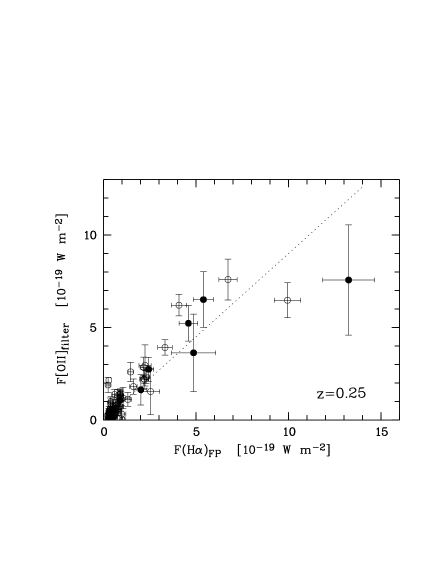
Figure 7: Extinction corrected [O ii] line fluxes plotted over the H$\alpha$ line fluxes for the galaxy sample at $z=0.25$. The mean ratio between both line fluxes is displayed by a straight line with $F$[O ii]/$F{\rm(H\alpha)}=0.9$. Filled circles indicate galaxies with $M_{\rm B}<-18.5$.

For galaxies seen in the light of H$\alpha$ at $z=0.25$, the [O ii] line fluxes are measured with the CADIS filter at $\lambda_{\rm c}=465$ nm. (see top of Table 1). In Fig. 7 the line fluxes are plotted for the galaxies with $(S/N)_{\rm[O\,II]}>1$. The average flux ratio results in $F{\rm[O\,II]}/F{\rm(H\alpha)}\sim 0.9$, in good agreement with the values cited above. This ratio is roughly in the mean of the ratios derived by Kennicutt (1998) and Sullivan et al. (2000).

Although there is a difference of roughly 4 Gyr between the epochs for $z=1.20$ and $z=0.25$, the line ratio may not have changed significantly. Based on the CFRS galaxy sample with redshifts in the range $0.5<z<1.0$, Carollo & Lilly (2001) found a remarkable similarity of metallicities to that for local galaxies. Also, Pettini et al. (1998) and Teplitz et al. (2000) found the line spectra at high redshift to be very similar to those observed in local emission line galaxies. The calibration used in the present study for the [O ii] emission is therefore

${\rm SFR}=0.88\times 10^{-34}L_{\rm[O\,II]}$   [M_⊙ yr^-1 W^-1].

Rosa-Gonzalez et al. (2002) derived SFR estimators using the Calzetti extinction curve and accounting for the underlying stellar Balmer absorption. Applying their calibration to our non-extinction corrected [O ii] galaxy sample we would end up with about two times higher star forming rates.

4.2 Star forming rates from the [O iii] $\lambda$500.7 line.

Having detected and measured a large number of [O iii] emission lines at medium redshift, we will test how far this prominent line can be used as SFR estimator.

The line luminosity functions for the galaxies observed in the [O iii] line at $z=0.40$ and $z=0.64$ are shown in Fig. 8. Again the distributions are fitted with Schechter functions, the parameters $\phi$ and $\alpha$ of which are taken from the $M_{\rm B}$ luminosity functions for the same redshift range (Fried et al. 2001).

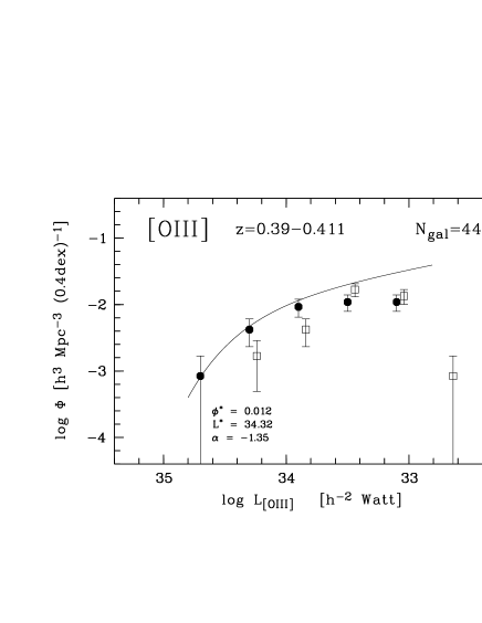
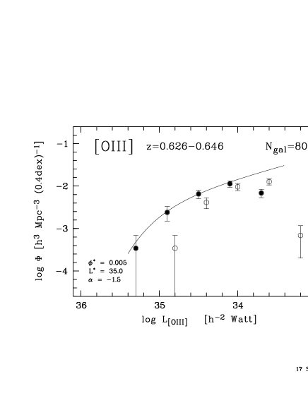
Figure 8: Luminosity functions for the [O iii] line emission at redshift 0.40 (top), and at redshift 0.64; open cirles are uncorrected, filled circles are extinction corrected values. Parameters for the Schechter function drawn are listed at the bright end of the LF.

Due to its high ionization level the luminosity of [O iii] 500.7 depends strongly on excitation and metallicity. In order to convert the [O iii] emission line luminosities into star formation rates, an averaged intensity ratio between H$\alpha$ and the ogygen line has therefore to be established. Since the population of galaxies may change with redshift, one has to use data sets measured at comparable redshifts for this.

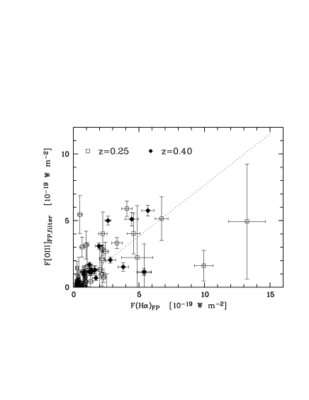
Figure 9: Extinction corrected [O iii] line fluxes plotted over the H$\alpha$ line fluxes for our galaxy sample at $z=0.25$ and at $z=0.40$; filled symbols are for galaxies with $M_{\rm B}<-18.5$ mag. The dotted line indicates the mean line ratio.

For the galaxies observed at $z=0.25$ in H$\alpha$, the extinction corrected fluxes for [O iii] 500.7 are plotted versus the H$\alpha$ fluxes as diamonds in Fig. 9. Also shown in this graph, as squares, are the corrected line flux data for a sample of star forming galaxies at $z=0.40$. At this redshift, the H$\alpha$ line happens to occur in the atmospheric C window at $\lambda\sim 918$ nm and, simultaneously, the [O iii] line in the A window at $\lambda\sim 702$ nm. Thus, the fluxes for both lines can be derived from FP scans rather accurately.

While the data points in the [O ii]/H$\alpha$ plot (Fig. 7) appear nicely correlated - in accordance with the well defined sequence in the diagnostic diagram [O ii] 372.7/[O iii] 500.7 vs. [O iii] 500.7/H$\beta$ (Baldwin et al. 1981) -, the data points in the H$\alpha$ vs. [O iii] flux diagram scatter considerably. The mean flux ratio determined from the global line emission densities is 0.76.

For the galaxies seen in [O iii] at $z=0.64$, the [O ii] line shows up in the medium band filter at 611 nm (see Fig. 1, second panel). The mean flux ratio derived from the global line emission densities of these galaxies is $F$[O iii]/$F$[O ii]$\approx 0.9$, in good agreement with the [O ii]/H$\alpha$ and [O iii]/H$\alpha$ ratios derived above.

We thus use for [O iii] the calibration:

${\rm SFR}=1.00\times 10^{-34}L_{\rm[O\,III]}$   [M_⊙ yr^-1 W^-1].

Table 4: Luminosity densities and star forming rates for the five lines and redshift intervals studied (for $H_{\rm 0}=70$ km sec^-1 Mpc^-1). L is given as sum of the observed fluxes, after extincion corrected, and after completeness correction.

z	Line	L   in 1032 W Mpc-3			SFR
		obs.	corr.	compl.	M⊙/Mpc3/yr
0.25	H$\alpha$	1.65	2.7	2.9	0.024$\pm$0.006
0.40	[OIII]	0.83	1.8	2.4	0.024$\pm$0.008
0.64	[OIII]	1.75	5.7	7.2	0.072$\pm$0.016
0.88	[OII]	2.00	7.5	12.2	0.107$\pm$0.035
1.20	[OII]	2.60	11.8	25.9	0.228$\pm$0.055

4.3 Completeness correction

Table 4 lists the line luminosity densities as observed by summing up the data after extinction correction and completeness correction, combined with the star forming rates for $H_{\rm 0}=70$ km sec^-1 Mpc^-1.

The completeness correction is done by calculating the area under the Schechter function according to:

${\rm SFR_{tot}}=\Phi^{\ast}\times L^{\ast}\times\Gamma(2+\alpha)$

A comparison between the SFR derived from the sum of the observed galaxy line emissions and the area under the Schechter function using the parameters marked in the plots shows that for the case of $z=0.25$, the completeness correction is negligible, while for the $z=1.2$ sample it amounts to a factor $>2$.

Small uncertainties in the slope parameters $\alpha$ may lead to large errors in the total luminosity and SFR. For $\alpha\sim 1.4$, which is the mean value in our curves, a variation of the slope parameter $\alpha$ by $\pm 0.1$ would alter the SFR by $\pm\sim 15\%$.

4.4 Evolution of SFR

The SFR values (Table 4) show an increase by about a factor of 10 between $z=0.25$ and $z=1.2$. This is in good agreement with the slope of the SFR data published by Hogg et al. (1998), who used the [O ii] line for all redshifts from 0.2 to 1.2, and with the slope derived from UV flux densities (Lilly et al. 1996).

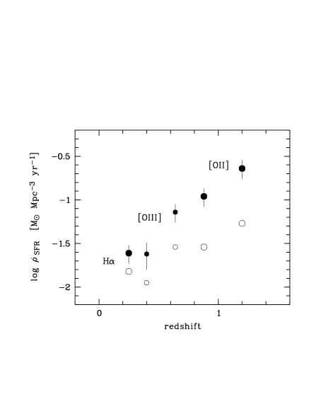
Figure 10: CADIS results for the completeness corrected star forming rate density as function of redshift. Large symbols are for H$\alpha$ ($z=0.25$) and [O ii] lines ($z=0.88,\leavevmode\nobreak\ 1.2$), small symbols (for [O iii] at $z=0.40$ and 0.64) are inserted for comparison. Filled circles stand for extinction-corrected, open ones for uncorrected values. Error bars are statistical.

As can be seen, the values at $z=0.88$ and 1.2 are rather sensitive to the extinction correction applied. The dispersion of $\pm 0.1$ in the reddening relation (Sect. 3.5) yields a systematic error bar of $\pm 40\%$ for both SFR values.

The SFR densities derived from the [O iii] line follow the trend of the other data within the errors. Using a large sample of galaxies and averaged line ratios, this line yields satisfactory results.

4.5 Field to field variation

Large scale structure expresses itself in strongly varying number counts from field to field and from redshift to redshift. This effect can nicely be seen in the $M_{\rm B}-z$ diagrams for the CADIS galaxies (Fried et al., 2001). Since the redshift intervals of our FP windows correspond roughly to the typical size of a LSS cell (50-100 Mpc), an even more distinct effect is expected here.

Indeed, the line luminosity density varies from field to field by a factor of about 2 (ratio of highest to lowest values for identical redshift intervals). An average over only three fields leaves an uncertainty of the order 40%.

4.6 Emission line luminosities versus UV luminosities

For optically selected galaxy samples the SFR can also be estimated by means of the UV emission. While the emission lines from H ii regions measure the rate of massive stars born less than a few million years ago, the integrated UV flux from short-lived stars indicates the star formation rate of a somewhat older star population. For large redshifts ($z>2.8$) where the observation of emission lines is extremely difficult and the L$\alpha$ line is often buried by internal dust extinction, Steidel et al. (1999) used the UV flux at 300 nm to derive star formation rates at high redshifts.

The conversion factor between UV flux and SFR is still a matter of debate and is sensitive to the metallicity and IMF used in the model calculation (Glazebrook et al. 1999), but also to the intrinsic dust extinction adopted.

We used for the extinction in the UV continuum the relation given by Calzetti et al. (1994):   ${\tau_{\rm B}}^{c}=0.5{\tau_{\rm B}}^{l}$,
where ${\tau_{\rm B}}^{c}$ and ${\tau_{\rm B}}^{l}$ are the optical depths for starlight continuum emission and for line emission from the H ii regions, respectively.

For the redshifts discussed above, the 280 nm (rest frame) continuum corresponds to observed wavelengths inbetween 350 nm and 616 nm. Except for the lowest redshift bin ($z=0.25$), the UV flux density at 280 nm can thus be easily determined from the CADIS multi-filter data. In the case of $z=0.25$, we use the 396 nm filter data if available, corresponding to a rest wavelength of 316 nm instead of 280 nm. To account for this wavelength difference, a correction factor of (280/316)² (corresponding to a flat spectrum $F_{\nu}=constant$) is applied to the UV flux densities.

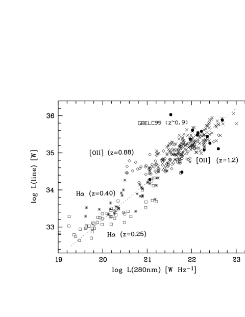
Figure 11: UV continuum flux density at 280 nm plotted versus emission line strengths, both reddening corrected, for redshifts between 0.25 and 1.2. Only objects with UV flux signal-to-noise ratios above 2 are shown here. The dotted line is for a Bruzual & Charlot model with solar abundance and Salpeter IMF and assuming the emission line galaxies are seen 0.1 Gyr after the star burst (Glazebrook et al. 1999).

The relation between UV continuum at 280 nm and emission line fluxes is shown in Fig. 11. In this graph, the [O ii] fluxes are scaled up by a factor 1.1 to account for the average line intensity ratio between H$\alpha$ and [O ii]. [O iii] line fluxes, which show a large scatter due to varying metallicity and excitation for individual galaxies, are not included; in the case of $z=0.4$, we however used the corresponding H$\alpha$ luminosities, measured in the atmospheric window C at 918 nm. The distribution shows no obvious deviation from proportionality over almost 4 decades, and it follows rather close the predictions from the Bruzual-Charlot model for solar abundance. Thus, the UV 280 nm continuum data for the CADIS galaxies are expected to yield a similar SFR as the line flux densities.

The CFRS galaxies at $z\sim 0.9$ studied by Glazebrook et al. (1999) (filled circles in the diagram) agree with our data. Their finding that the mean star formation rate derived their from H$\alpha$ data is three times as high as the ultraviolet estimates seems to become obsolete when the reddening correction proposed in a footnote in their table 2 is applied (1.6 for H$\alpha$ and of 3.1 for $L(280)$, almost identical with the corrections applied in the present paper and with the reddening correction proposed by Steidel et al., 1999). The remaining offset to higher luminosities of the Glazebrook galaxies as compared to our $z=0.88$ sample is due to the fact that the CFRS survey covers a larger volume than the present study, but is less deep in terms of emission line luminosities.

Sullivan et al. (2000, 2001) did a similar comparison based on a UV selected sample of galaxies in a redshift range $0<z<0.4$. They also find agreement with the Glazebrook et al. (1999) data for the bright end of the sample. At the faint end, however, the UV fluxes are too high as compared to the H$\alpha$ line emission, not explainable by insufficient dust extinction correction. Sullivan et al. explain this discrepancy by series of starbursts superimposed on underlying quiescent star formation of the galaxies. Interestingly our emission line selected galaxy samples show an effect in the opposite direction (taking each redshift bin separately), which can be explained by exactly the same effect. Whereas an emission line selected galaxy sample prefers those (faint) galaxies which just happen to be in a starburst phase, a UV selected sample preferentially selects those which are in a state about 10⁸ years past their starburst.

4.7 Comparison with other studies

In Fig. 12, our values are inserted in a diagram similar to that presented by Glazebrook et al. (1999), with the lookback time as abscissae, showing the optical SFR values as well as those derived from FIR/sub-mm and UV luminosities. Here, all SFR values from UV studies are corrected by factors between 2.7 and 4.5, depending on the rest wavelength observed, but irrespective the galaxy brightnesses. This extinction correction is based on a global value $E_{\rm B-V}=0.15$, as proposed by Steidel et al. (1999). Note that this value corresponds to an emission line extinction correction with $E_{\rm B-V}=0.3$ (Calzetti et al. 1994), typical for a $M_{\rm B}=20$ mag galaxy. The diagram shows that with this correction the different approaches to determine the SFR lead to satisfactorily consistent distributions (the error bars do not include systematic errors).

While our SFR values for redshift below 1.0 are close to those published by other authors, our value at $z=1.2$ seems to be significantly higher, probably due to the greater depth of the CADIS survey.

It is remarkable how closely the SFR data from infrared and sub-mm observations follow those derived from optical observations, although IRAS and ISO observations show that a notable part of the IR radiation density arises from galaxies barely visible in the optical, such as ULIRGs and AGNs. This agreement expresses the consistency of the conversion factors for the different kind of data, and the plausibility of the corrections to be applied. A close agreement between SFR densities derived from different wavelength regimes was also presented by Rosa-Gonzalez et al. (2002), who used global factors for the extinction correction of the luminosity densities, independent of redshift.

The increase of the star forming rate with lookback time in Fig. 12 can be well described by SFR$\propto exp(t_{\rm lookback}/2.6)$ (dotted line), with the lookback time given in Gyrs. This exponential relation fits better than the power law $(1+z)^{3.9}$ fit proposed by Lilly et al. (1996) for the UV luminosity evolution.

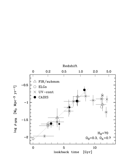
Figure 12: SFR density vs. redshift. CADIS points at $z=0.25$, 0.4, 0.64, and 1.2 (black dots) are inserted in this diagram adopted from figure 8 of Glazebrook et al. (1999). UV data are from Sullivan et al. (2000), Lilly et al (1996), Connolly et al. (1997) and Madau et al. (1996), FIR and sub-mm data from Flores et al. (1999), and Hughes et al. (1998), emission line data from Gallego et al. (1995) at $z=0$, Tresse & Maddox (1998), Glazebrook et al. (1999), and Pettini et al. (1998). UV values are extinction corrected according to Steidel et al. (1999). Literature SFR values are transformed to the cosmology used in the the present paper (parameters in the lower right of the figure). The dotted line represents a hand-drawn fit to the data.

While the UV fluxes are closely correlated to the emission line luminosities, irrespective the redshift (Fig. 11), the flux density in the blue decreases by a factor of only $\sim 4$ between $z=1$ and today, compatible with passive evolution (Fried et al. 2001). Comparing the $M_{\rm B}^{\ast}$ values from Fig. 5 with the corresponding $L^{\ast}$ values marked in Fig. 6 (both Schechter functions have the identical $\phi$ and $\alpha$ parameters), one can see, that the ratio between blue flux density and emission line flux density (star formation rate) increases by a factor $\sim 5$ between $z=0.25$ and 1.2. Thus, the star forming rate per blue luminosity unit increases drastically with time. The slower evolution of the blue luminosity density indicates that the relation between moderately young stars (age $\simeq 2$ Gyr) to very young stars (age $\la 0.1$ Gyr) evolves with time in that sense that a higher redshift starbursts were more frequent than today.

Two interpretations are possible for the exponential decay of the SFR. One is that on average the amount of gas available in the galaxies determines the SFR and thus young galaxies have larger star forming activities. The other interpretation is that independent of the gas content, a high star forming activity is induced by galaxy-galaxy interactions. In this case the interpretation would be that more interactions must have occurred at high redshifts. Both of these could have an exponential decay with time. The latter interpretation is supported by LeFevre et al. (2000) who find an increase of the interaction rate with $(1+z)^{2.7}$, resulting in a factor 8 between today and $z=1.2$. Model calculations show that an exponential law fits perfectly to the merger rates (Khochfar et al. 2003).

5 Conclusions

Based on the photometric emission line data the star formation rates for redshifts ranging from 0.25 and 1.2 are derived. This CADIS emission line survey used for the present study survey is deeper than similar studies performed up to now and thus the resulting luminosity densities and star formation rates are less affected by the completeness correction of the luminosity functions. All results, including broad band colors, are based on only one data set.

The SFR increases by $\sim 20$ from $z=0$ to $z=1.2$, following an exponential relation ${\rm SFR}\propto exp(t_{\rm lookback}/2.6)$.

The (blue) luminosity functions derived from the line emission galaxy samples agree well with those derived from the multi-color survey of CADIS at comparable redshifts. Also, the emission line luminosity functions agree in shape ($\Phi^{\ast}$ and $\alpha$) with the corresponding blue magnitude luminosity functions, although $L^{\ast}_{\rm lines}$ evolves $\sim 5$ times faster than $M_{\rm B}^{\ast}$ within the studied redshift range of $z=0.25$ to 1.2.

A steep rise of SFR with lookback time up to 8 Gyrs is clearly indicated, and can well described with an exponential decay of SFR with time, with a (half) decay time of $\sim 2.6$ Gyrs.

The extinction correction plays an important role in the determination of the SFR and leads to major (systematic) uncertainties; for higher redshifts, where the Balmer line ratio cannot be determined accurate enough, the correction can be only carried out with global methods. A reddening correction depending on absolute magnitude leads to consistent results.

- (1) Baldwin, J.A., Phillips, M.M., & Terlevich, R. 1981, PASP, 93, 5
- (2) Bell, E.F., & Kennicutt, R.C. 2001, ApJ, 548, 681
- (3) Bertin, E., & Arnouts, S, 1996, A&A, 117, 393
- (4) Carollo, C.M., & Lilly, S.J. 2001, ApJ, 548, L53
- (5) Connolly, A.J., Szalay, A.S., Dickinson, M., Subbarao, M.U., & Brunner, R.J. 1997, ApJ, 486, L11
- (6) Cowie, L.L., Hu, E.M., Songaila, A., & Egami, E. 1997, ApJ, 481, L9
- (7) Calzetti, D., Kinney, A.L., & Storchi-Bergmann, T. 1994, ApJ, 429, 582
- (8) Flores, H., Hammer, F., T. Thuan, T., et al. 1999, ApJ, 517, 148
- (9) French, H. 1980, ApJ, 240, 41
- (10) Fried, J.W., von Kuhlmann, B., Meisenheimer, et al. 2001, A&A, 367, 788
- (11) Gallagher, J.S., Bushouse, H., & Hunter, D.A. 1989, AJ, 97, 700
- (12) Gallego, J., Zamorano, J., Aragon-Salamanca, A., & Rego, M. 1995, ApJ, 455, L1
- (13) Gallego, J., Zamorano, J., Rego, M., Alonso, O., & Vitores, A.G. 1996, A&AS, 120, 323
- (14) Gallego, J., Zamorano, J., Rego, M., & Vitores, A.G. 1997, ApJ, 475, 502
- (15) Glazebrook, K., Blake, C., Economou, F., Lilly, S., & Colless, M. 1999, MNRAS, 306, 843
- (16) Hammer, F., Flores, H., Lilly, S.J., et al. 1997, ApJ, 481, 49
- (17) Ho, L.C., Filippenko, A.V., & Sargent, W.L.W. 1997, ApJS, 112, 315
- (18) Hogg, D.W. Cohen, J.G., Blandford, R., & Phare, M.A. 1998, ApJ, 504, 622
- (19) Hughes, D.H., Serjeant, S., Dunlop, J., et al. 1998, Nature, 394, 241
- (20) Jansen, R.A., Franx, M., & Fabricant, D. 2001, ApJ, 551, 825
- (21) Kennicutt, R.C. 1983, ApJ, 272, 54
- (22) Kennicutt, R.C. 1992, ApJ, 388, 310
- (23) Kennicutt, R.C. 1998, ARA&A, 36, 189
- (24) Khochfar, S., et al. 2003, in preparation
- (25) Kinney, A.L., Calzetti, D., Bohlin, R., et al. 1996, ApJ, 467, 38
- (26) LeFevre, O., Abraham, R., Lilly, S., L., et al. 2000, MNRAS, 311, 565
- (27) Lilly, S.J., Le Fèvre, Hammer, F.O., & Crampton. D. 1996, ApJ, 460, L1
- (28) Madau, P., Ferguson, H.C., Dickinson, M., et al. 1996, MNRAS, 283, 1388
- (29) Maier C., Meisenheimer, K., Hippelein, H., et al. 2003, submitted
- (30) McCall, M.L., Rybski, P.M., & Shields, G.A. 1985, ApJS, 57, 1
- (31) Meisenheimer, K., & Röser, H.-J. 1993, in Landolt-Börnstein, Extension and Supplement to Volume 2, Subvolume a, 29 (Springer Verlag)
- (32) Meisenheimer, K., Fried, J.W., Hippelein, H., et al. 2002, in preparation
- (33) Pettini, M., Kellogg, M. Steidel, C.C., et al. 1998, ApJ, 508, 539
- (34) Pettini, M., Shapley, A.E., Steidel, C.C., et al. 2001, ApJ, 554, 981
- (35) Popescu, C.C., & Hopp, U. 2000, A&AS, 142, 247
- (36) Rosa-Gonzalez, Terlevich, E., & Terlevich, R. 2002, MNRAS, 332, 283
- (37) Rowan-Robinson, M., Mann, R.G., Oliver, S.J., et al. 1997, MNRAS, 289, 490
- (38) Steidel, C.C., Adelberger, K.L., Giavalisco, M., et al. 1999, ApJ, 519, 1
- (39) Szokoly, G., et al., 2002, A&A, submitted
- (40) Sullivan, M., Treyer, M.A., Ellis, R.S., et al. 2000, MNRAS, 312, 442
- (41) Sullivan, M., Mobasher, B., Chan, B., et al. 2001, ApJ, 558, 72
- (42) Teplitz, H.I., Malkan, M.A., Steidel, C.C., et al. 2000, ApJ, 542, 18
- (43) Terlevich, R., Melnick, J., Masegosa, J., et al. 1991, A&AS, 91, 285
- (44) Tresse, L., & Maddox, S.J. 1998, ApJ, 495, 691
- (45) Veilleux, S., & Osterbrock, D.E. 1987, ApJS, 63, 295
- (46) Vogel, S., Engels, D., Hagen, H.-J., et al. 1993, A&AS, 98, 193
- (47) Wolf, C., Meisenheimer, K., Röser, H.-J., et al. 2001, A&A, 365, 681
- (48) Yan, L., McCarthy, P.J., Freudling, W., et al. 1999, ApJ, 519, L47